8 - 1

Chapter 8. Sources of Extraneous Variability

Understanding VariabilitySystematic Variance

Systematic Error (Confounding)

Random Error

Sources of Extraneous VariabilityParticipants as a Source of Extraneous Variability

Experimenter as a Source of Extraneous Variability

Method as a Source of Extraneous Variability

Thinking Critically About Everyday Information

Validity of the Research DesignInternal Validity

External Validity

Case Analysis

General Summary

Detailed Summary

Key Terms

Review Questions/Exercises

8 - 2

Understanding VariabilityIn this chapter, we will deal with three very important concepts: systematic variance (also called between

group variance), systematic error (also called confounding), and random error (also called within-group

variance or error variance). As a general rule, we want to maximize systematic variance, minimize

random error, and eliminate systematic error.

When we make observations and measure dependent variables, there will undoubtedly be variability

in the scores that we obtain. That is, not all of the participants’ scores will be the same. Let’s try to

understand the reasons why their scores are not all the same. Assume that we have two groups of children.

One group watches a television program without violence, and another group watches a television

program with violence. We then allow the children to play on the playground, and we observe the number

of aggressive behaviors that each child exhibits. We obtain the data shown in Table 8.1.

Systematic Variance

Clearly, there is variability in these scores. Why didn’t each child show the same number of

aggressive behaviors? One possible source of variability is the systematic variance that results

from the treatment effect. This is the variability that we hypothesized would occur as a result of our

manipulation of the independent variable (level of TV violence). Systematic variance contributes to and

helps explain the difference or variability between participant scores in the two groups, and therefore the

difference between the two group means.

8 - 3

Systematic Error (Confounding)

The difference between the two group means could also be due to factors other than the independent

variable. These other factors cause systematic error and are often referred to as confounding variables,

or confounds. Systematic error relates to internal validity, which we discuss at the end of the chapter.

The hallmark of a good experimental method or procedure is that you allow to vary only one factor

(IV) at a time and everything else is held constant. Then if you observe a systematic change in behavior,

you know that the change is due to your IV. If everything else is held constant, no alternative (rival)

explanations are needed for your findings. However, if the method did allow one or more factors to vary

along with the IV, then you would not know which factor caused the change in the observed behavior.

Whenever more than one factor at a time varies, you have confounding. For example, if you had

asked the group of 20 children for 10 volunteers to watch Mister Rogers (nonviolent) and 10 volunteers to

watch Beast Wars (violent), is it possible that the two groups differed even before you presented the TV

program? Is it possible that those children who elected to watch Beast Wars were more aggressive to

begin with? In this case, it would not be possible to separate the effects of your independent variable from

differences in aggression that result from self-selection to the groups. Is it possible that you, the

experimenter, were more likely to rate a behavior as aggressive if you knew that the child had just

finished watching Beast Wars? These issues, along with several others, are discussed in more detail

below.

Remember that confounding variables affect the scores in one group differently than the scores in

another group. Sources of systematic error affect the variability between the groups. If they increase

variability in the same direction as the hypothesized effect of the independent variable, you may falsely

conclude that your treatment had an effect when, in fact, the difference was a result of systematic error. If

there is an increase in the opposite direction, you may falsely conclude that your treatment had no effect

when, in fact, the effect was masked by systematic error.

Random Error

So, confounds result in alternative interpretations (rival hypotheses) of the data and make an

unambiguous interpretation of the findings difficult. They can also affect, along with other factors, the

variability of scores between the groups. Other extraneous variables affect the variability of scores within

the groups. Why didn’t each child who watched Mister Rogers exhibit the same number of aggressive

behaviors on the playground? Why didn’t each child who watched Beast Wars exhibit the same number

of aggressive behaviors? Some sources of random error are obvious. These are different children with

different backgrounds. You expect them to be different. Other factors may not be so obvious. Did some or

all of the children know that they were being watched on the playground? Did the level of personality

8 - 4

development vary? Age? Number of males and females? The number of siblings each participant had?

Each of these factors could have affected behavior—that is, caused behavior to vary from person to

person. Is it possible that the experimenter experienced lapses in attention and missed some aggressive

behaviors? The fact that these extraneous variables increase the variability of scores within the groups

makes it more difficult for the experimenter to discover sources of systematic variance between groups

resulting from manipulation of the independent variable.

Thus, behavioral research presents the interesting challenge of attempting to discover sources of

systematic variability while simultaneously attempting to eliminate sources of systematic error

(confounds) and reduce (minimize) random error. Although there is no perfect experiment, an experiment

can be evaluated in terms of how well it answers the questions that are asked. If they can be answered

unambiguously, without either qualifying comments or the availability of alternative explanations, the

experiment may be considered unusually good. We will now explore extraneous variables in more detail.

Sources of Extraneous VariabilityExtraneous variables should be evaluated both when planning research and when evaluating the results

after the data have been collected. Some extraneous variables can be anticipated; others are revealed

during the course of the experiment. Those that are anticipated can often be addressed by using specific

experimental design techniques (discussed in the next chapter). Those that are revealed during the

experiment aid in interpretation of the research findings.

Sources of extraneous variability can be categorized into the areas of research participants,

experimenter, and method (experimental design). Table 8.2 provides an overview of the various sources

of extraneous variability and includes some of the relevant questions that should be asked during both

design and evaluation of research. Note that some of these extraneous variables are more likely to be

confounds that contribute to systematic error, whereas others are more likely to contribute to random

error. Each should be evaluated on both counts. Also, keep in mind that identifying a possible source of

confounding is much more important than labeling or categorizing it. The label itself is unimportant.

Indeed, different individuals may place a possible source of confounding in different categories.

8 - 5

Participants as a Source of Extraneous Variability

History. Whenever a measure is taken more than one time in the course of an experiment—that is,

pre- and posttest measures—variables related to history may play a role. Specific events occurring

between the first and second recordings may affect the dependent variable. The longer the time period

8 - 6

between the measurement periods and the less control over the participants (degree of isolation) during

this period, the greater is the likelihood that these factors will affect the participants.

Let’s consider an example involving our TV violence question. On a Tuesday morning, we show the

children at a day-care center a TV program with violence and then observe their behavior during

playtime. The following Tuesday, we show the same group of children a nonviolent TV program and

again observe their behavior during playtime. We find that the children showed fewer aggressive

behaviors during the second observation period. We also know that the day after the first observation the

day-care center hired a new, and much stricter, director. This new director is a potential confound because

this person could have affected the children’s behavior in one condition but not the other. We do not

know whether the change in children’s behavior is due to the independent variable (type of TV program)

or this confounding variable (new director).

Maturation. With history, specific events occur that are often external to the participants and are

largely accidental. Similar to history are maturational events. However, maturation is a developmental

process within the individual. Included under maturational events are such factors as growth, fatigue,

boredom, and aging. Indeed, almost all biological or psychological processes that vary as a function of

time and are independent of specific events may be considered maturational factors. On occasion, it is

difficult to determine whether to classify an observation in one category or another. As we noted, this is

not a matter of concern. The important thing is to recognize that other factors besides the independent

variable may be considered as a rival explanation for behavioral change.

On Tuesday, we show our group of children a two-hour movie that includes violence and then put

them in a playroom for two hours for observation of aggressive behavior. We do the same on the

following Tuesday but show a two-hour movie that does not include violence. If these are young children,

can we expect all of them to sit still for two hours and watch a movie? If they get distracted after a short

period of time, then we are not really manipulating our independent variable. Likewise, during the

observation period, will they get bored being in the same playroom with the same toys? Could this

boredom affect their level of aggressive behavior? Could this boredom affect one condition more than the

other?

Attrition. In Chapter 2, we pointed out that human participants must be permitted to withdraw from

an experiment at any time. Some will exercise this option. Some may withdraw for reasons of illness,

others because they do not find the research to their liking. In animal studies, some participants may die

and others become ill. Some attrition, in and of itself, is not serious. However, confounding may occur

when the loss of participants in the various comparison groups is different, resulting in the groups’ having

different characteristics. This type of confound is referred to as differential participant attrition.

8 - 7

For example, a group of children, with consent from their parents, take part in a three-month study to

assess the effect of TV violence on aggressive behavior. The experimenter randomly assigns half of the

children to watch nonviolent TV programs and the other half to watch TV programs that contain some

violence. As we will see in the next chapter, by randomly assigning participants to each condition we

assume that the groups are equal on all characteristics. Random assignment is the best way that we know

of to form equal groups on all known and unknown factors. During the course of the three months,

approximately one-fourth of parents whose children have been assigned to watch TV violence reconsider

their consent and decide to withdraw their children from the study. During the course of the three months,

there is no attrition in the nonviolent group. Clearly, this will reduce the sample size in one of the groups.

More important, the differential attrition could be a confound. It is possible that the parents most

concerned about the welfare of their child would have children who tend to be less aggressive. Thus, you

may not only be losing participants from one of the groups, you may be losing participants with specific

characteristics related to the dependent variable. Therefore, what started out as equal groups in the two

conditions ends up as two very different groups.

Let’s look at another example. Imagine that a research team is interested in comparing the traditional

lecture approach to instruction with the Personalized System of Instruction (PSI), in which each student

works at his or her own pace. They randomly assign students to lecture or PSI sections. The students

assigned to the lecture method will serve as a comparison group for students assigned to the PSI method.

A pretest on abilities at the beginning of the school term shows that the characteristics of students in the

two instructional conditions are comparable. As is true in all classes, students drop courses for a variety of

reasons as the term goes on. At the end of the school term, a common final exam is given to all students

in the lecture and PSI sections. It is found that the PSI students do much better than the lecture students.

However, the research team kept careful records of those who dropped out of the different instructional

sections. It was found that more students of low ability dropped from the PSI than from the lecture

sections. Consequently, the comparison between the lecture method and the PSI method was confounded.

Not only did the method of instruction differ, but because of differential attrition, the abilities of students

also differed. Because of this confounding, the actual differences obtained could be due to differences in

instructional methods or to differences between high-ability students in PSI and lower-ability students in

the lecture sections.

Particularly vulnerable to the effects of attrition are developmental and follow-up studies. The loss

of participants in itself, though unfortunate, does not lead to differential bias or confounding.

Confounding occurs when subjects with certain kinds of characteristics tend to be lost in one group but

not another. To avoid drawing a faulty conclusion, it is important to keep careful records. It must be

possible to document and assess the loss of participants.

8 - 8

Demand Characteristics. Different situations “demand” different behavior patterns. The behavior

of people in church is very different from their behavior at a football game, or when they are at their place

of employment. Similarly, the behavior of students in classroom situations is typically different from their

nonclassroom behavior. These behavior patterns may vary with the size and type of class and

characteristics of the instructor. Thus, situations tend to “call out” or “demand” expected behavior

patterns. Experimental settings are similar. It is possible that the implicit and explicit cues found in

research settings may be responsible for the observed behavior rather than the independent variable. If

this is the case, we have compromised the integrity of the study. We must remain aware that the very act

of measuring behavior may change the behavior measured.

The implicit and explicit cues surrounding the experiment, referred to as demand characteristics,

may consist of the instructions given, the questions asked, the apparatus used, the procedures, the

behavior of the researcher, and an almost endless variety of other cues. Cues from these various sources

allow participants to speculate about the purpose of the experiment and the kind of behavior that is ex-

pected of them.

Demand characteristics can have different effects. They may lead participants to form hypotheses—

either correct or incorrect—about the nature of the experiment. Some participants may react in a

compliant way to “help” the experimenter’s efforts, whereas others may react in a defiant way to “hinder”

the experimenter’s efforts. Still other participants may simply perform in a way they think is expected of

them. Whatever the case, demand characteristics can affect the quality of the experiment.

For example, the children in our TV violence study may not behave naturally during the observation

period because they know that they are part of a study. As a result, they “perform” for the researchers

based on what they believe the researchers expect of them. Some studies actually demonstrate demand

characteristics. One such study investigated the acceptance of rape myths (for example, that women have

more control in a rape situation than is actually the case) in both men and women (Bryant, Mealey,

Herzog, & Rychwalski, 2001). The Rape Myth Acceptance Scale was given to young adults at a shopping

mall. Half the time the researcher was dressed provocatively, and half the time the researcher was dressed

conservatively. Results showed that rape myths were more accepted (by both men and women) when the

researcher was dressed conservatively, and the researchers attributed this effect to demand characteristics.

Note that such an effect could also be labeled experimenter effects. Again, the particular label is not the

critical point.

Before describing how demand characteristics can be detected and their effects minimized, we should

note that participants are generally conscientious when participating in research. There is little evidence

that most participants are either compliant (giving “right” data) or defiant (giving “wrong” data).

Although we cannot ignore demand characteristics, we should not become unduly concerned about

them to the point of pessimism concerning research. Debriefing is one common method used to assess

8 - 9

demand characteristics. Debriefing can include a postexperimental questionnaire aimed at discovering

how participants interpreted the situation—their perceptions, beliefs, and thoughts of what the experiment

was about. This information can reveal whether demand characteristics were operating. The researcher

must be careful that the questions do not guide the participant. Otherwise, the answers to the

questionnaire are themselves a component of demand characteristics. To obtain useful information, the

investigator should use open-ended questions followed up by probing questions.

In the long run, the most valid way of ascertaining whether demand characteristics posed a problem

is to evaluate the extent to which the results generalize. If the results generalize to other situations,

laboratory or nonlaboratory, then demand characteristics that restrict our conclusions to a specific

experimental setting were not operating.

Evaluation Apprehension. Participants entering the laboratory bring with them a variety of

concerns and motivations. The laboratory setting, as we have seen, leads to demand characteristics, but it

also leads to concern and apprehension about being evaluated. Many participants become particularly

concerned about doing well or making a good impression. Under these circumstances, they may become

sensitive and eagerly seek out cues from the experimenter. After the experimental session is over, the

floodgates are open for a flow of questions: “How did I do?” “Did I pass?” “I didn’t make a fool of

myself, did I?”

The participant’s evaluation apprehension, or fear of being judged, leads to several problems. One

we have noted already: Participants tend to be especially eager for cues from the experimenter. It is also

possible that one treatment, in an experiment having several, may give rise to greater apprehension or

concern about being judged than the others. If this happens, we then have the problem of confounding. By

differentially arousing suspicion among participants in an experiment, we have, in fact, created different

conditions over and above the treatment condition. Anything in an experiment that arouses suspicion that

a participant is being judged can create these difficulties.

Diffusion of Treatment. Some of the preceding factors can be magnified if participants learn about

details of the experiment before they participate. This can occur inadvertently by overhearing a

conversation about the experiment. More often, a friend or college classmate who has already participated

informs the future participant. This is particularly problematic when the experiment involves some degree

of deception in order to elicit natural behavior. If diffusion of treatment is a concern, it is wise to take a

minute at the end of each experimental session to request that participants not discuss the experiment with

others who might be participants in the future.

8 - 10

Experimenter as a Source of Extraneous Variability

Experimenter Characteristics. The personality and physical characteristics of the experimenter are

often overlooked as sources of extraneous variability. Many of the factors just discussed, including

attrition, demand characteristics, and evaluation apprehension can be affected by experimenter

characteristics. The way that the experimenter interacts with the participants can increase or decrease the

degree to which these other factors become extraneous variables. It is important for the experimenter to

act like a professional. The more serious the experimenter is about the study, the more serious the

participants will be. An experimenter who dresses in shabby clothes, appears unprepared, and jokes

around with participants runs the risk of increased random error from participants who do not take their

role seriously.

There is also evidence that physical characteristics of the experimenter can be an extraneous

variable. Think about it. Can your behavior be affected by the gender, attractiveness, age, or race of the

person you are interacting with? Of course it can, and the same is true in the experimental situation where

the participant interacts with the researcher. We have already mentioned a study in which the dress of the

experimenter influenced participant responses on the Rape Myth Acceptance Scale. Other studies have

shown that gender (Barnes & Rosenthal, 1985; Friedman, Kurland, & Rosenthal, 1965), attractiveness

(Barnes & Rosenthal, 1985; Binder, McConnell, & Sjoholm, 1957), age (Ehrlich & Riesman, 1961), and

race of the experimenter (Katz, Robinson, & Epps, 1964) can affect scores on the dependent variable.

This is not to say that these factors will serve as extraneous variables in all, or even most, studies. Their

possible effect will depend on the particular variables manipulated and measured in the study. The point

is that the researcher should consider these as possible sources of extraneous variability in both the design

and evaluation phases of research.

Experimenter Bias. One of the great myths about scientists is that they are aloof, objective, un-

biased, and disinterested in the outcomes of their research. They are interested in one thing and one thing

only—scientific truth. Although objectivity is a goal toward which to strive, in actual fact many if not

most scientists fall considerably short of the mark. Indeed, they have made a considerable personal invest-

ment in their research and theoretical reflections. They passionately want their theories confirmed in the

crucible of laboratory or field research. The very intensity of their desires and expectations make their

research vulnerable to the effects of experimenter bias. Two major classes of experimenter bias are (1)

errors in recording or computation and (2) experimenter expectancies that are unintentionally

communicated to the experimental participants.

Recording and computational errors do not affect the participant’s behavior. Generally unintentional,

they may occur at any phase of the experiment, such as when making observations, transcribing data, or

analyzing results. If the errors are random, then no problem exists. It is when the errors are systematic that

8 - 11

real problems develop. We mentioned earlier in this chapter that an experimenter making observations of

children may be more likely to record a behavior as aggressive if the experimenter knows that this child

just finished watching the TV program with violence.

The second class of experimenter effects do affect the participant’s performance. These are often

referred to as experimenter expectancies. Here, the behavior desired by the experimenter is

unintentionally communicated to the participant. Perhaps one of the most interesting illustrations of

experimenter expectancy is the story of Clever Hans. Clever Hans was a horse owned by a schoolteacher

named von Osten during the 1800s. Clever Hans developed a reputation for solving various mathematical

problems. If Clever Hans was asked the product of 3 × 3, he would stomp with one of his hoofs nine

times. Similar feats were routinely performed. Interestingly, von Osten believed that Hans actually

possessed advanced mathematical ability and invited scientific inquiry into the abilities of the horse.

Detailed and painstaking research revealed that Hans was able to perform as billed, but only under

specific conditions.

The individual posing the problem had to be visibly present while the answer was being given, and

he or she had to know the answer. For example, if the questioner thought that the square root of 9 was 4,

Hans would answer “four.” You may have guessed that the experimenter (questioner) unintentionally

communicated the desirable behavior (correct answer) to the participant (Clever Hans). It was later

determined that Clever Hans was a very ordinary horse, but one that had developed an uncanny ability to

respond to slight visual cues. It seems that when a question was asked, the questioner tilted his head

forward to look at Hans’ leg and hoof. When the correct number of stomps occurred, the questioner then

looked up. This was a cue to Hans to stop “counting.” How the horse learned this difficult discrimination

probably relates to operant conditioning and reinforcement principles.

How expectancies may affect behavior in an experimental setting is illustrated in a series of studies

that investigated the effect of teacher expectancies on student performance in the classroom. In an early

and well-known study, Rosenthal and Jacobson (1968) gave an intelligence test to students in grammar

school. They then told the teachers that some of the students were “late bloomers” and that these children

would show considerable improvement over the year. In fact, the children described as late bloomers

were chosen randomly and were no different from the others. The effect of this label was apparently

dramatic. When those identified as late bloomers were later retested, their mean score was much higher

than that of other children who were not labeled late bloomers. Although some researchers have been

critical of the methodology used in this early study, the basic effect has been supported.

We can speculate how teachers might treat children labeled as “bright” or “slow.” Those carrying the

bright label might be given more attention, more encouragement, and greater responsibilities. In short,

teachers’ expectations probably affect the way they interact with students. The quality of this interaction

may help or hinder a student, depending on a teacher’s expectations. This is one reason why some

8 - 12

educators are opposed to systems of education that segregate students on the basis of ability testing. In

such systems, educators would have different expectations of students, thereby affecting the way the

students are treated and what is expected of them. These expectations might, in turn, affect the students’

performance. Some have called this process a self-fulfilling prophecy. Such effects have been

demonstrated between teachers and gifted children in the classroom (Kolb & Jussim, 1994),

experimenters and participants performing a psychomotor task (Callaway, Nowicki, & Duke, 1980), and

coaches and athletes (Solomon, 2002).

To sum up, studies have demonstrated experimenter expectancies in various settings. Although these

studies designate experimenter expectancy as an independent variable, the danger is that the behavior of

participants in many studies could be unknowingly affected by experimenter expectancies. In such

studies, quality is jeopardized. The observed effects represent a confounding of experimenter expectancy

and experimental treatment.

Method as a Source of Extraneous Variability

Selection. In a typical experiment, groups are selected to receive different levels of the independent

variable. To conclude that this manipulation caused differences in the dependent variable, the researcher

must be confident that the groups were not selected in a way that created differences in the dependent

variable before the independent variable was even introduced. That is, the researcher must be confident

that the groups were equivalent to begin with. A researcher would not want children with aggressive

personalities in the group that watches violent TV and children with nonaggressive personalities in the

group that watches nonviolent TV (or vice versa). Any differences in behavior between the two groups

could be due to either the independent variable (level of TV violence) or the way in which children were

assigned to the groups. In other words, selection would be a confound. In the next chapter, we will

discuss design methods to avoid this problem. There are also statistical methods that can adjust for initial

differences between groups.

Task and Instructions. The task is what participants have to do so that we can measure our

dependent variable. If we are interested in reaction time as a dependent variable, do the participants press

a telegraph key, or release it, or do we measure it in some other way? If we are interested in reading rate,

what material does the participant read? How is it read? Subvocally? Aloud? If we want to measure

aggressive behavior, do we ask children to play on a playground? Play in a room full of toys? In an

experimental study, it is essential that participants in all groups perform identical tasks. If we knowingly

or unknowingly vary both the independent variable and the task, any observed differences between

groups could be due to the independent variable or to the different tasks they performed.

8 - 13

Sometimes task confounding is so obvious that we have no difficulty recognizing it. For example, we

would not observe aggressive behavior on the playground for one group and in a room full of toys for the

other group. Likewise, we would not compare gasoline consumption of two different makes of

automobiles of the same size and power by calculating the miles per gallon of one car on a test track and

the other one in real traffic. If we were interested in comparing individuals’ ability to track a moving

target while experiencing two types of distraction, we would want the target being tracked to move at the

same speed for both types. The only thing that should vary is the type of distraction. In these examples,

task confounding can be easily seen. However, on some occasions, task confounding is so subtle that it is

difficult to recognize. To illustrate, researchers were interested in the effects certain colors have on

learning words. They prepared a list of ten five-letter words. Five of the ten words were printed in red,

and five were printed in yellow. Twenty students were randomly selected from the college population and

given the list of words to learn. All participants learned the same list. The criterion for learning was two

perfect recitals of the ten-word list. Results showed that words printed in red were learned more rapidly

than those printed in yellow. On the surface, it appears that the speed of learning was a function of the

color of the printed words. Before drawing this conclusion, however, we should ask, “Was the task the

same for the different colored words?” A few moments’ reflection should produce a negative reply. Why?

Because different words appeared in the red as opposed to the yellow condition, the tasks were different.

This suggests a possible alternative interpretation of the findings—namely, that the five words printed in

red were easier words to learn, independent of the color used. This problem could have been avoided by

using a different procedure. Instead of all participants’ having the same five words printed in red and the

other five words printed in yellow, a different set of words could have been randomly chosen for each

participant, of which five were printed in red and five in yellow.

The following example describes a case of task confounding so subtle that many experts would miss

it. Folklore has it that the more frequently you test students, the more they learn. Imagine that instructors

of introductory psychology courses are interested in improving learning in various sections of the course.

One obvious possibility is to increase the frequency of testing. Before doing so, however, they must

assure themselves that the folklore is correct. Consequently, they design a study to test the “frequency of

testing” hypothesis.

Many classes of 40 students each are available for research. Students and instructors are randomly

assigned to courses that are to be tested different numbers of times. The researchers decide to give some

students nine tests, others six tests, and still others three tests. Only introductory sections are used, with an

equal number assigned to each test frequency. The same book and chapter assignments are used. Further,

all instructors select test questions from the same source book. All tests contain 50 multiple-choice items.

Grades on each exam are based on percentages: more than 90% correct, an A; 80%, a B; 70%, a C; 60%,

8 - 14

a D. The results are clear and statistically significant: the more frequent the tests, the better the

performance. Are there alternative interpretations to the frequency of testing hypothesis?

If each test contained 50 items, the number of items differed from condition to condition. Thus, the

nine-test condition received 450 items during the semester; the six-test condition received 300 items; and

the three-test condition received 150 items. In other words, the three conditions varied in the number of

items received during a semester as well as in the number of tests. The treatment condition was therefore

confounded with task differences. To avoid this problem, the researchers could have limited the number

of questions to 180 and then given nine tests each with 20 questions; six tests with 30 questions, and three

tests with 60 questions. This way, the total number of items would be constant while allowing frequency

of testing to vary. But a problem still remains. If the researchers allow a full hour for each test, then the

nine-test groups receiving only 20 questions could spend as much as three minutes per item, the six-test

groups with 30 questions about two minutes, and the three-test groups with 60 questions only about one

minute. The investigators could give everyone only one minute per test question, giving the nine-, six-,

and three-test frequency groups 20, 30, or 60 minutes, respectively. This is somewhat better, but task con-

founding is still present if fatigue is a factor or warm-up time is necessary. The problems encountered

here are excellent examples of the difficulties involved in doing well-controlled research.

When human participants are used, instructions in some form are necessary to inform the

participants about what the task is. If they are to perform the task in the way that the experimenter wants

them to, then the instructions must be clear. If unclear, instructions may result in greater variability in

performance among participants, or worse, they may result in participants’ performing different tasks.

The task would vary depending on the level of understanding of the instructions. It is essential when

using complex instructions to evaluate their adequacy before beginning the experiment. It is not unusual

for instructions to go through several modifications before they are etched in stone. Even then, the

post-experimental interview might reveal that portions of the instructions were unclear for some

participants.

Testing Effects. Researchers sometimes find it necessary to give a pretest and a posttest. The pretest

is given before and the posttest after the experimental treatment. Presumably, any differences that occur

between the pre- and posttests are due to the treatment itself. However, a possible rival explanation is that

the pretest accounts for the results; that is, there was something about taking the pretest that affected

scores on the posttest. There is a substantial body of evidence showing such testing effects. Individuals

frequently improve their performance the second time they take a test; on occasion, the opposite may be

found. The test may be a comparable test, an alternate form of the same test, or actually the same test.

Because these changes in performance occur without any experimental treatment, it is important to assess

them and to use the proper controls (these controls will be discussed later in the book). Many researchers

8 - 15

have expressed concern that the process of measuring apparently changes that which is measured. We are

not yet sufficiently knowledgeable to know the reasons why this may be so. Pretests may sensitize

participants to selectively attend to certain aspects of the experiment simply by the nature of the questions

asked. Therefore, changes observed on posttests may be largely due to pretests’ alerting or guiding the

participant.

Carryover Effects. Testing effects can occur when a participant has prior experience with the test.

Carryover effects involve a more general issue whereby prior experience in an experimental condition

(or conditions) affects behavior in a subsequent condition (or conditions). Thus, carryover effects are a

concern whenever the research design requires data collection from each participant in two or more

sequential conditions. At times, participation in an initial condition will alert the participant to the

purposes of the study and, thereby, influence their behavior in later phases of the research. At other times,

simple practice with a task leads to better performance in subsequent conditions. A more detailed

discussion of carryover effects, including the research design techniques to address them, is presented in

Chapter 12.

Instrumentation. The term instrumentation encompasses a class of extraneous variables larger

than the word implies. It includes not only physical instrumentation (electrical, mechanical, and the like)

but also human observers, raters, or scorers. In much research, repeated observations are necessary. Any

changes in performance between the first and all following observations may be due to changes in your

measuring instrument—physical or human. Raters or observers may become more skillful in identifying

certain behaviors, but they may also become fatigued or bored.

As an experimenter, you may be nervous at the beginning of the experiment and much more relaxed

after you become accustomed to your participants and procedure. When handling animals, you may be

initially timid, tentative, and somewhat uneasy. With experience and familiarity, your handling techniques

improve. Grading essay exams poses a problem for instructors at times. The criteria for evaluation may

change in a gradual and systematic fashion between the start and completion of the task. Papers read

earlier may have either an advantage or disadvantage, depending on the direction in which the criteria

change.

Because psychologists must frequently rely on raters or observers, the problem of accurate and

reliable measuring techniques is important. Minimizing changes in these measurements requires careful

training of observers. As we noted in Chapter 6, some investigators use more than one rater or observer

and then calculate, periodically, the extent to which (1) different observers or recorders agree with one

another (interobserver or interrecorder reliability) or (2) the same observers or recorders agree with

themselves at different times (intraobserver or intrarecorder reliability). Because some shifts are almost

8 - 16

inevitable, it is wise to randomly assign the experimental treatment to the available experimental session.

For example, if all participants in one condition are seen first, and those in another condition are seen

second, the treatment effects are confounded with possible systematic chances in instrumentation.

Regression to the Mean. Let us imagine that you have developed a procedure you believe will

alleviate chronic depressive disorders. You administer a depression scale to large numbers of people. As

your treatment group, you select a group drawn from those who obtained the highest depression scores.

Subsequently, you administer the experimental treatment and find a significant improvement in their

scores on the depression scale. Can you conclude that the treatment was effective?

This study is typical of many pilot research programs that report exciting initial results that are not

substantiated by later, better-designed studies. It suffers from vulnerability to the regression phenomenon:

Whenever we select a sample of participants because of their extreme scores on a scale of interest and test

them again at a later date, the mean of the sample on these posttest scores typically moves closer to the

population mean. This occurs whether the extremes are drawn from the low end or high end of the scale.

This movement of the extremes toward the center of the distribution is known as regression to the mean.

There is nothing mysterious about this phenomenon. Whenever performance is exceptional, a number of

factors combine to produce this unusual outcome. Many of these factors are temporary and fleeting. They

are what statisticians refer to as chance variables. If these variables combine in such a way as to lower

performance at a given time, it is unlikely that they will repeat themselves the next time. Thus, the

individual will appear to improve. On the other hand, an exceptionally good performance has enjoyed the

confluence of many favorable chance factors. It is unlikely that these will repeat themselves on the next

occasion. Thus, the individual will appear to get worse.

In short, regression to the mean is a function of using extreme scores and imperfect measuring

instruments. The more extreme the scores and the lower the reliability of the instrument, the greater will

be the degree of regression. For example, let’s say that we are interested in whether the effect of TV

violence depends on the prior level of aggressive behavior in the child. So we want to select one group of

children who are nonaggressive and another group of children who are already very aggressive. To do

this, we observe a large number of children on the playground and select for the experiment those

children who showed no aggressive behavior and those who showed high levels of aggressive behavior.

Both groups watch the TV program with violence, and then we observe them again on the playground.

We find that the nonaggressive children now show some aggressive behavior and that the aggressive

children now show lower levels of aggressive behavior. These may be interesting findings, suggesting

that the effect of TV violence depends on the prior aggressive nature of the child; or these findings may

simply represent the effect of regression to the mean. Because the two groups were selected for being at

8 - 17

the extremes, regression to the mean would predict that their behavior would moderate to the center at a

second observation setting.

Regression is a statistical phenomenon and is not due to any experimental treatment. Therefore, if

we select participants who score extremely low on a pretest and then give them a posttest (same test)

without introducing a treatment of any kind, participants would be expected to perform higher on the

posttest. The reverse of this is true for extremely high scores; that is, participants should perform lower on

the posttest. When a treatment condition is added between the pre- and posttests, investigators often

confuse regression to the mean with the treatment effect and wrongly conclude that the treatment was

effective.

Let’s consider a few more examples. I have just completed grading my midterm exam in my

Research Methods course. The results were very disappointing, and I now have to improve the

performance of at least some of the students. I am especially concerned with those doing very poorly.

During the remainder of the term, I introduce a number of new teaching procedures, carefully keeping a

record of each. After the final exam, I immediately compare the midterm and final exam scores of those

who were doing very poorly. I find that the mean score of this group has increased. My satisfaction is

enormous. This new teaching technique and its accomplishments should be shared with my academic

colleagues. Question: Is this enthusiasm justified? Probably not. As the instructor, I might be very

unhappy and disappointed if I were to compare the midterm and final grades of those doing extremely

well in the course. I would probably find that my most brilliant students did not perform as well on the

final as they did on the midterm. Again, regression to the mean rather than the new teaching method may

be responsible.

For any given year, we select 50 active baseball players with the poorest hitting

records and calculate their mean batting average. In this group of 50 ballplayers, we will have some who

are not very good hitters, and they will always remain in this category of poorest hitters. However, there

are also those who are much better hitters than the current year’s batting averages reflect. They will no

doubt improve their hitting the next year. The batting average of these better players may have been

reduced because of injury, illness, changing batting stance, dissatisfaction with play, unhappiness with

teammates, playing a new position, or other temporary reasons. These factors lead to error variance; that

is, they result in an imperfect correlation between their batting record in one year and in the subsequent

year. It is this second group of players who will move the mean batting average upward to the mean. The

two essentials are present for regression to the mean: extreme scores, and imperfect correlation between

pre and post measures due to error factors. Improvements in the overall batting average (regression to the

mean) may also be aided by those players who deserve to be in the “poorest hitter” category. If you

assume that their average is so low that it cannot go lower (floor effect), then the only way they can

change at this extreme is to improve.

8 - 18

Another example from sports also illustrates regression to the mean. Those of you who play golf will

appreciate this. The weekend is here and you have a tee time for 18 holes of golf at one of your favorite

courses. The day is sunny and warm with no wind to speak of. You had a good night’s sleep and are

feeling very good. It has not rained for several days, and the fairways are hard and give the ball lots of

roll. They have watered the greens so that they are soft and hold well. Your tee shots for the day cut the

middle of the fairway and you hit every green with your approach in regulation play. Your putting, like

your woods and iron, is as good as it has ever been, and every event that happens seems to go your way. It

turns out that your score is the best you have ever had. The question is, How will your golf score compare

the next time that you play? Why?

Take a look at the box “Thinking Critically About Everyday Information,” and consider the issue of

extraneous variables in a news report regarding the link between smoking in films and teenage smoking.

8 - 19

Thinking Critically About Everyday Information: Smoking in Movies and Smoking in Teenagers

Several news organizations reported the results of a large study that examined the link between cigarette smoking depicted in movies and the number of teenagers who start smoking. Portions of the report that appeared in USA Today are printed below:

Study: Smoking in Movies Encourages TeensLONDON (AP) — Youngsters who watch movies in which actors smoke a lot are three

times more likely to take up the habit than those exposed to less smoking on-screen, a new study of American adolescents suggests. The study, published Tuesday on the Web site of The Lancetmedical journal, provides the strongest evidence to date that smoking depicted in movies encourages adolescents to start smoking, according to some experts. Others said they remain unconvinced. Many studies have linked smoking in films with increased adolescent smoking, but this is the first to assess children before they start smoking and track them over time. The investigators concluded that 52% of the youngsters in the study who smoked started entirely because of seeing movie stars smoke on screen. . . .

However, Paul Levinson, a media theorist at Fordham University in New York noted there are many reasons people start smoking and the study could not accurately determine how important each factor is. “It’s the kind of thing we should be looking at but . . . the fact that two things seem to be intertwined doesn’t mean that the first causes the second,” said Levinson, who was not involved in the study. “What we really need is some kind of experimental study where there’s a controlled group.” . . .

The research, conducted by scientists at Dartmouth Medical School, involved 2,603 children from Vermont and New Hampshire schools who were aged between 10 and 14 at the start of the study in 1999 and had never smoked a cigarette at the time they were recruited. The adolescents were asked at the beginning of the study which movies they had seen from a list of 50 movies released between 1988 and 1999. Investigators counted the number of times smoking was depicted in each movie and determined how many smoking incidents each of the adolescents had seen. Exposure was categorized into four groups, with the lowest level involving between zero and 531 occurrences of smoking and the highest involving between 1,665 and 5,308 incidents of smoking. There were about 650 adolescents in each exposure group.

Within two years, 259, or 10%, of the youths reported they had started to smoke or had at least taken a few puffs. Twenty-two of those exposed to the least on-screen smoking took up the habit, compared with 107 in the highest exposure group—a fivefold difference. However, after taking into account factors known to be linked with starting smoking, such as sensation-seeking, rebelliousness or having a friend or relative who smokes, the real effect was reduced to a threefold difference.

Think about the following questions:• Can you identify possible extraneous variables in this study? Actually, several potential sources of

systematic error are mentioned in the report. What are they?• If people just read the title of the report, would they get the impression that smoking in the movies at

least partially causes teenage smoking? Do you believe that this is misleading? Do you agree with the comments of Paul Levinson?

• Can you think of a more accurate title for the article?

SOURCE: Retrieved June 10, 2003, online at http://www.usatoday.com/news/health/2003-06-09-teen-smoking_x.htm

8 - 20

Validity of the Research DesignAs we have noted, extraneous variables negatively impact the quality of research. In

Chapter 5, we introduced the concept of validity—an assessment as to whether you are studying what you

believe you are studying. Several specific types of validity are often used to assess qualities of an

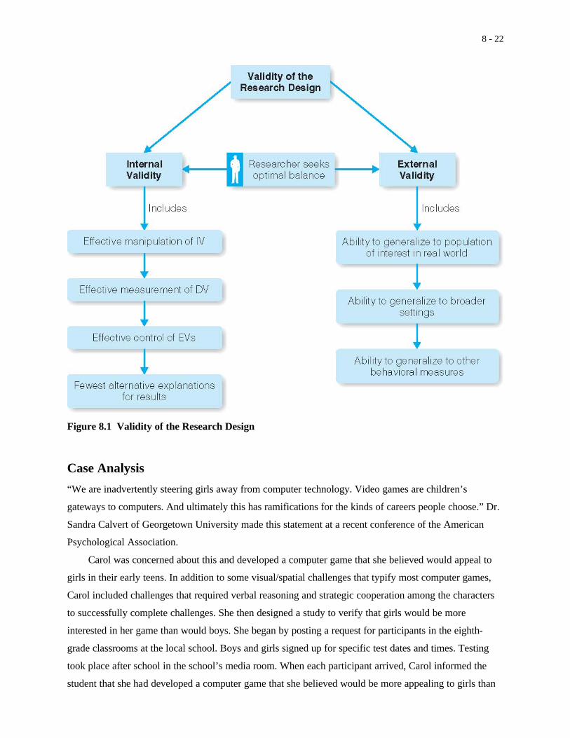
experimental design. Internal validity considers the degree to which there was an effective manipulation

of the independent variable and an effective measurement of the dependent variable, and the degree to

which sources of extraneous variability were eliminated or controlled. External validity considers the

degree to which the results of the study will generalize from the specific sample and conditions of the

experiment to the more general population and more general conditions of the real world.

Internal Validity

Extraneous variables that contribute to random error or are confounds and contribute to systematic error

are undesirable. Whenever they occur, we compromise the internal validity of the experiment. We cannot

be sure whether a lack of significant results is due to no effect of the independent variable, to systematic

error, or to too much random error. We cannot be sure that an observed relationship is between our

independent and dependent variables, because other factors also varied concurrently with the independent

variable. The relationship obtained could be due to confounding variables. As we noted earlier, when

confounding occurs, the relationship that we observe is open to alternative interpretations. It is important

to note that the mere suspicion of confounding is sufficient to compromise internal validity. The burden

of ruling out the possibility of extraneous factors rests with the experimenter. The greater the number of

plausible alternative explanations available to account for an observed finding, the poorer is the

experiment. Conversely, the fewer the number of plausible alternative explanations available, the better

the experiment is. As we shall see, true experiments that are properly executed rule out the greatest

number of alternative hypotheses.

External Validity

Another form of validity, referred to as external validity, deals with generalizing our findings. We want

to design our research so that our findings can be generalized from a small sample of participants to a

population, from a specific experimental setting to a much broader setting, from our specific values of an

independent variable to a wider range of values, and finally, from a specific behavioral measure to other

behavioral measures. The greater the generality of our findings, the greater is the external validity. It

should be clear by now that if an experiment does not have internal validity, then it cannot have external

validity. Other threats to external validity can include specific characteristics of the laboratory setting and

the particular characteristics of the participants used.

8 - 21

The laboratory setting usually involves the research participant in an unfamiliar environment,

interacting with unfamiliar people. In some cases, this can lead to observed behaviors that are different

from those that would be observed in the real world. Consider little Johnny who is in our TV violence

study. Let’s assume that we design our study such that Johnny arrives at the university research center

along with the other children who were randomly sampled, is randomly assigned to be with a particular

group of unfamiliar children who watch an unfamiliar TV program with violence, watches the program

in an unfamiliar room, goes to another unfamiliar room to play with the unfamiliar children and the

unfamiliar toys that are present, and is observed by an unfamiliar adult. Will we observe natural

behavior? Will Johnny behave as if he had just watched the show at home and then gone to his room to

play with friends?

Generally, the greater the degree of experimental control, the more concern there must be with

external validity. The challenge to the researcher is to maximize the degree of experimental control

(internal validity) while designing a testing environment that will result in natural behavior that can be

generalized to nonexperimental settings (external validity). However, we should note that some

laboratory experiments are interested in testing a specific hypothesis under highly controlled conditions

and not too interested in generalizing the data for that study. In this case, internal validity is paramount,

and external validity is less of an issue.

External validity is also related to the particular sample of participants used. In the last chapter, we

discussed the importance of obtaining a representative sample from a well-defined population. It is

important to return to this in our discussion of external validity and to focus on the issues of age, gender,

race, and cultural differences. For many years, the typical human participant in behavioral research was a

young, white, adult American male. Too often, these research findings were translated into general

theories of human behavior without due consideration of the relatively narrow population from which

participants were drawn. In more recent years, researchers have examined how these participant

characteristics can affect results, and there is an increased emphasis on diversity when selecting

participants for a study. However, there continues to be a preponderance of human research in which the

participants are white, American college students. Again, it is important for the researcher to realize the

population from which participants are sampled and to avoid overgeneralization beyond that population.

Figure 8.1 summarizes the components that determine the validity of a research design.

8 - 22

Figure 8.1 Validity of the Research Design

Case Analysis“We are inadvertently steering girls away from computer technology. Video games are children’s

gateways to computers. And ultimately this has ramifications for the kinds of careers people choose.” Dr.

Sandra Calvert of Georgetown University made this statement at a recent conference of the American

Psychological Association.

Carol was concerned about this and developed a computer game that she believed would appeal to

girls in their early teens. In addition to some visual/spatial challenges that typify most computer games,

Carol included challenges that required verbal reasoning and strategic cooperation among the characters

to successfully complete challenges. She then designed a study to verify that girls would be more

interested in her game than would boys. She began by posting a request for participants in the eighth-

grade classrooms at the local school. Boys and girls signed up for specific test dates and times. Testing

took place after school in the school’s media room. When each participant arrived, Carol informed the

student that she had developed a computer game that she believed would be more appealing to girls than

8 - 23

to boys and that she was testing this research question. Carol decided to measure the participants’ interest

in the game in two ways. First, she sat adjacent to each participant at the computer and rated, at five-

minute intervals, the perceived interest of the participant. Second, she asked each participant, at the end of

the session, to rate on a Likert scale their interest in the computer game.

The testing went well except that one-third of the boys had to withdraw from the experiment early to

attend football practice. Carol summarized the data and was happy to note that both the experimenter

ratings and participant ratings showed that the girls were more interested in the computer game than the

boys.

Critical Thinking Questions

1. Describe at least six potential sources of extraneous variability in Carol’s study.

2. For each source identified, describe a more effective methodology that would reduce or eliminate that

source of extraneous variability.

3. What other aspects of the study could be improved?

General SummaryThe heart of behavioral research design is an understanding of the sources of variability in behavior and

an understanding of how to manipulate or control those sources of variability. Systematic variability

explains differences in behavior that result from manipulation of the independent variable. The researcher

attempts to maximize systematic variability. Extraneous variability represents differences in behavior

that result from systematic error (confounds) and random error. The researcher attempts to eliminate

systematic error and to minimize random error.

Sources of extraneous variability include participants (history, maturation, attrition, demand

characteristics, evaluation apprehension, diffusion of treatment), experimenter (experimenter

characteristics, experimenter bias), and method (selection, task and instructions, testing effects, carryover

effects, instrumentation, regression to the mean). The degree to which systematic variability is

established and extraneous variability (error) is minimized relates directly to the internal validity of the

study. Internal validity is necessary but not sufficient to ensure external validity, whereby the researcher

can generalize the results to a particular population of individuals. In the next chapter, we will focus on

experimental control techniques that are designed to reduce both systematic error and random error and,

thus, to increase internal and external validity.

Detailed Summary1. Variability in participant scores is often the result of systematic variance, systematic error, and

random error. Systematic variance is due to any treatment effect (IV); systematic error is due to

8 - 24

extraneous variables (confounds) that affect scores between groups; random error is due to

extraneous variables that affect scores within groups.

2. Extraneous variables should be evaluated both when planning research and when evaluating the

results after the data have been collected.

3. Sources of extraneous variability can be categorized into the areas of participants, experimenter, and

method.

4. Participant sources of extraneous variability include history, maturation, attrition, demand

characteristics, evaluation apprehension, and diffusion of treatment.

5. History is the occurrence of an event during the course of the experiment that affects participant

behavior. Maturation includes short-term and long-term changes in the state of participants that affect

behavior. Attrition is the loss of participants during the course of the study. Demand characteristics

are the expectations for certain behaviors that participants experience as a result of the study.

Evaluation apprehension is the uncomfortable feeling that participants may experience and that may

affect behavior. Diffusion of treatment occurs when initial participants inform later participants about

specifics of the study.

6. Experimenter sources of extraneous variability include experimenter characteristics and experimenter

bias.

7. Experimenter characteristics are the personality and physical characteristics of the experimenter that

affect participant behavior. Experimenter bias includes expectations by the experimenter that

influence the recording or scoring of data, as well as the unintended communication of expectancies

to participants that may affect their behavior.

8. Method sources of extraneous variability include selection, task and instructions, testing effects,

instrumentation, and regression to the mean.

9. Selection is an issue when the groups are selected in a way that creates differences in the dependent

variable before the independent variable is even introduced. Task and instructions are issues when

participants do not perform identical tasks during measurement of the dependent variable or do not

receive identical instructions. Testing is an issue when prior measurements (pretest) influence

subsequent measurements (posttest). Instrumentation is an issue when the criteria for measurement

by physical instruments or human observers change during the course of the experiment. Regression

to the mean is an issue when groups are formed based on extreme scores.

10. The validity of a research design is synonymous with the quality of the study and consists of both

internal validity and external validity.

11. Internal validity of a study includes effective manipulation of the independent variable, effective

measurement of the dependent variable, effective control of extraneous variables, and the ability to

eliminate alternative explanations for the results.

8 - 25

12. External validity of a study includes the ability to generalize from the sample to the population of

interest, the ability to generalize to broader settings, and the ability to generalize to other behavioral

measures.

Key Terms attrition

carryover effects

confounding variables (confounds)

demand characteristics

diffusion of treatment

evaluation apprehension

experimenter bias

experimenter characteristics

experimenter expectancies

external validity

history

instructions

instrumentation

internal validity

maturation

random error

regression to the mean

selection

systematic error (confounding)

systematic variance

task

testing effects

Review Questions / ExercisesA psychology student is interested in whether involvement in aerobic exercise improves mood more than

involvement in nonaerobic exercise. He decides to study a group of university students who have

enrolled in a Bowling course for the fall semester. At the beginning of the semester, he gives them a

mood scale to complete. At the end of the semester, he again gives them the mood scale to complete. He

8 - 26

asks that all the participants enroll in a Jogging course for the spring semester. He gives them the mood

scale again at the end of the spring semester.

1. What method of sampling was used?

2. Evaluate the study in terms of each source of extraneous variability listed in Table 8.2. For each

source, explain why or why not you believe that it is a design issue. If you believe that it is a design

issue, explain whether it is a source of systematic error or random error.

3. How would you rate the internal validity of the study—good, fair, or poor? Explain.

4. How would you rate the external validity of the study—good, fair, or poor? Explain.