CHAPTER 8 Hashing

Instructor: C. Y. Tang

Ref.: Ellis Horowitz, Sartaj Sahni, and Susan Anderson-Freed, “Fundamentals of Data Structures in C,” Computer Science Press, 1992.

Concept of Hashing

In CS, a hash table, or a hash map, is a data structure that associates keys with values.

Look-Up Table Dictionary Cache Extended Array

Tables of logarithms

Example

A small phone book as a hash table.(Figure is from Wikipedia)

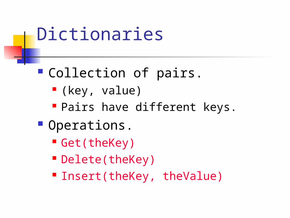
Dictionaries

Collection of pairs. (key, value) Pairs have different keys.

Operations. Get(theKey) Delete(theKey) Insert(theKey, theValue)

Just An Idea

Hash table : Collection of pairs, Lookup function (Hash function)

Hash tables are often used to implement associative arrays, Worst-case time for Get, Insert, and

Delete is O(size). Expected time is O(1).

Origins of the Term

The term "hash" comes by way of analogy with its standard meaning in the physical world, to "chop and mix.” D. Knuth notes that Hans Peter Luhn of IBM appears to have been the first to use the concept, in a memo dated January 1953; the term hash came into use some ten years later.

Data Structure for Hash Table

#define MAX_CHAR 10#define TABLE_SIZE 13typedef struct { char key[MAX_CHAR]; /* other fields */} element;element hash_table[TABLE_SIZE];

Other Extensions

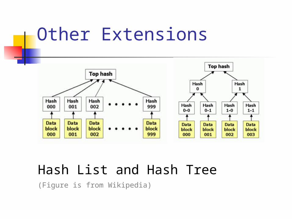
Hash List and Hash Tree(Figure is from Wikipedia)

Formal Definition

Hash Function In addition, one-to-one /

onto

The Scheme

Figure is from Data Structures and Program Design In C++, 1999 Prentice-Hall, Inc.

Ideal Hashing

Uses an array table[0:b-1]. Each position of this array is a bucket. A bucket can normally hold only one

dictionary pair. Uses a hash function f that converts

each key k into an index in the range [0, b-1].

Every dictionary pair (key, element) is stored in its home bucket table[f[key]].

Example

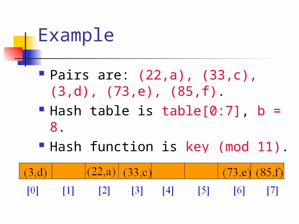
Pairs are: (22,a), (33,c), (3,d), (73,e), (85,f).

Hash table is table[0:7], b = 8. Hash function is key (mod 11).

What Can Go Wrong?

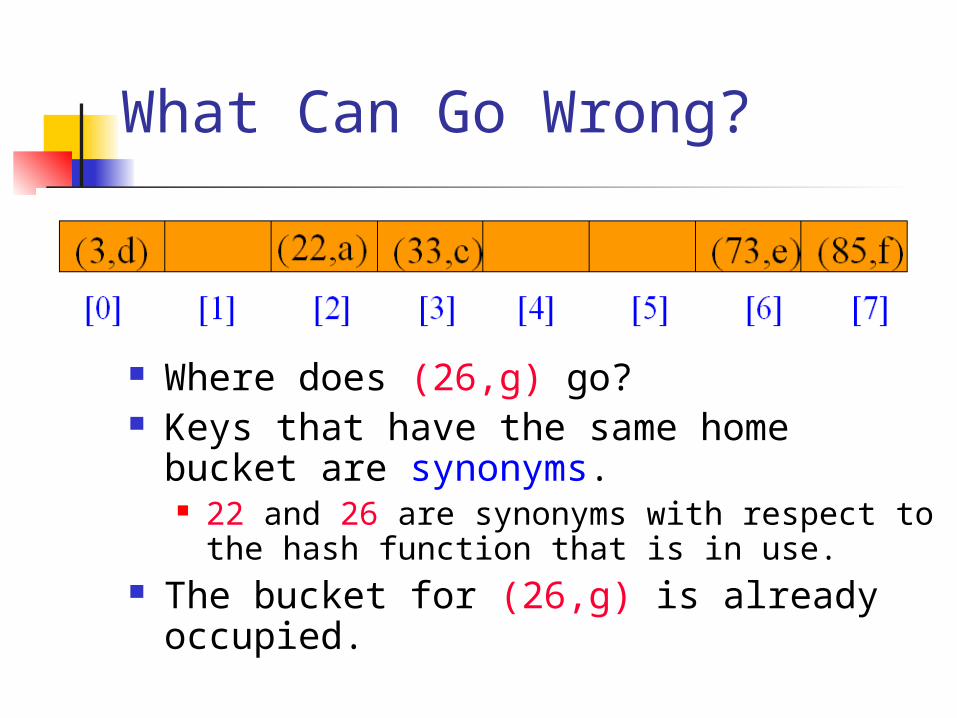
Where does (26,g) go? Keys that have the same home bucket

are synonyms. 22 and 26 are synonyms with respect to the

hash function that is in use. The bucket for (26,g) is already occupied.

Some Issues

Choice of hash function. Really tricky! To avoid collision (two different pairs

are in the same the same bucket.) Size (number of buckets) of hash table.

Overflow handling method. Overflow: there is no space in the

bucket for the new pair.

Example Slot 0 Slot 1

0 acos atan12 char ceil3 define4 exp5 float floor6…25

synonymssynonyms:char, ceil, clock, ctime

overflow

synonyms

Choice of Hash Function

Requirements easy computation minimal number of collisions

If a hashing function groups key values together, this is called clustering of the keys.

A good hashing function distributes the key values uniformly through the range.

Some hash functions

Middle of square H(x):= return middle digits of x^2

Division H(x):= return x (mod k)

Multiplicative: H(x):= return the first few digits of the

fractional part of x*k, where k is a fraction.

advocated by D. Knuth in TAOCP vol. III.

Some hash functions II

Folding: Partition the identifier x into several parts,

and add the parts together to obtain the hash address, e.g., x=12320324111220

Partition x into 123,203,241,112,20; And return the address 123+203+241+112+20=699

Digit analysis: If all the keys have been known, then we

could delete the digits of keys having the most skewed distributions, and use the rest digits as hash address.

Hashing By Division

Domain is all integers. For size of hash table b, the number

of integers that get hashed into bucket i is approximately 232/b.

The division method results in a uniform hash function which means it maps the keys into buckets such that approximately the same number of keys get mapped into each bucket.

Hashing By Division II

In practice, keys tend to be correlated. divisor is an even number, odd

integers hash into odd home buckets and even integers into even home buckets.

20%14 = 6, 30%14 = 2, 8%14 = 8 15%14 = 1, 3%14 = 3, 23%14 = 9

divisor is an odd number, odd (even) integers may hash into any home.

20%15 = 5, 30%15 = 0, 8%15 = 8 15%15 = 0, 3%15 = 3, 23%15 = 8

Hashing By Division III

Similar biased distribution of home buckets is seen, in practice, when the divisor is a multiple of prime numbers such as 3, 5, 7, …

The effect of each prime divisor p of b decreases as p gets larger.

Ideally, choose b so that it is a prime number.

Alternatively, choose b so that it has no prime factor smaller than 20.

Hash Algorithm via Division

void init_table(element ht[]){ int i; for (i=0; i<TABLE_SIZE; i++) ht[i].key[0]=NULL;}

int transform(char *key){ int number=0; while (*key) number += *key++; return number;}

int hash(char *key){ return (transform(key) % TABLE_SIZE);}

Criterion of Hash Table

The key density of a hash table is the ratio n/T n is the number of keys in the table T is possible keys

The loading density or loading factor of a hash table is = n/(sb) s is the number of slots b is the number of buckets

Example Slot 0 Slot 1

0 acos atan12 char ceil3 define4 exp5 float floor6…25

b=26, s=2, n=10, =10/52=0.19, f(x)=the first char of x

synonymssynonyms:char, ceil, clock, ctime

overflow

synonyms

Overflow Handling

An overflow occurs when the home bucket for a new pair (key, element) is full.

We may handle overflows by: Search the hash table in some systematic

fashion for a bucket that is not full. Linear probing (linear open addressing). Quadratic probing. Random probing.

Eliminate overflows by permitting each bucket to keep a list of all pairs for which it is the home bucket.

Array linear list. Chain.

Linear probing (linear open addressing) Open addressing ensures that all

elements are stored directly into the hash table, thus it attempts to resolve collisions using various methods.

Linear Probing resolves collisions by placing the data into the next open slot in the table.

Linear Probing – Get And Insert

divisor = b (number of buckets) = 17. Home bucket = key % 17.

0 4 8 12 16

• Insert pairs whose keys are 6, 12, 34, 29, 28, 11, 23, 7, 0, 33, 30, 45

6 12 2934 28 1123 70 333045

Linear Probing – Delete

Delete(0)

0 4 8 12 166 12 2934 28 1123 70 333045

0 4 8 12 166 12 2934 28 1123 745 3330

• Search cluster for pair (if any) to fill vacated bucket.

0 4 8 12 166 12 2934 28 1123 745 3330

Linear Probing – Delete(34)

Search cluster for pair (if any) to fill vacated bucket.

0 4 8 12 166 12 2934 28 1123 70 333045

0 4 8 12 166 12 290 28 1123 7 333045

0 4 8 12 166 12 290 28 1123 7 333045

0 4 8 12 166 12 2928 1123 70 333045

Linear Probing – Delete(29)

Search cluster for pair (if any) to fill vacated bucket.

0 4 8 12 166 12 2934 28 1123 70 333045

0 4 8 12 166 1234 28 1123 70 333045

0 4 8 12 166 12 1134 2823 70 333045

0 4 8 12 166 12 1134 2823 70 333045

0 4 8 12 166 12 1134 2823 70 3330 45

Performance Of Linear Probing

Worst-case find/insert/erase time is (n), where n is the number of pairs in the table.

This happens when all pairs are in the same cluster.

0 4 8 12 166 12 2934 28 1123 70 333045

Expected Performance

= loading density = (number of pairs)/b. = 12/17.

Sn = expected number of buckets examined in a successful search when n is large

Un = expected number of buckets examined in a unsuccessful search when n is large

Time to put and remove governed by Un.

0 4 8 12 166 12 2934 28 1123 70 333045

Expected Performance

Sn ~ ½(1 + 1/(1 – )) Un ~ ½(1 + 1/(1 – )2) Note that 0 <= <= 1.The proof refers to D. Knuth’s TAOCP

vol. III

alpha Sn Un

0.50 1.5 2.5

0.75 2.5 8.5

0.90 5.5 50.5

<= 0.75 is recommended.

Linear Probing

void linear_insert(element item, element ht[])

{

int i, hash_value;

I = hash_value = hash(item.key);

while(strlen(ht[i].key)) { if (!strcmp(ht[i].key, item.key))

fprintf(stderr, “Duplicate entry\n”);

exit(1);

}

i = (i+1)%TABLE_SIZE;

if (i == hash_value) {

fprintf(stderr, “The table is full\n”);

exit(1);

}

}

ht[i] = item;

}

Problem of Linear Probing

Identifiers tend to cluster together Adjacent cluster tend to coalesce Increase the search time

Coalesce Phenomenon

bucket x bucket searched bucket x bucket searched

0 acos 1 1 atoi 22 char 1 3 define 14 exp 1 5 ceil 46 cos 5 7 float 38 atol 9 9 floor 510 ctime 9 …… 25

Average number of buckets examined is 41/11=3.73

Quadratic Probing

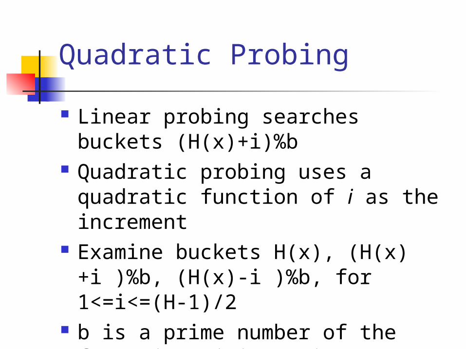
Linear probing searches buckets (H(x)+i)%b

Quadratic probing uses a quadratic function of i as the increment

Examine buckets H(x), (H(x)+i )%b, (H(x)-i )%b, for 1<=i<=(H-1)/2

b is a prime number of the form 4j+3, j is an integer

Random Probing

Random Probing works incorporating with random numbers. H(x):= (H’(x) + S[i]) % b S[i] is a table with size b-1 S[i] is a random permuation of

integers [1,b-1].

Rehashing

Rehashing: Try H1, H2, …, Hm in sequence if collision occurs. Here Hi is a hash function.

Double hashing is one of the best methods for dealing with collisions. If the slot is full, then a second hash

function is calculated and combined with the first hash function.

H(k, i) = (H1(k) + i H2(k) ) % m

Summary: Hash Table Design

Performance requirements are given, determine maximum permissible loading density. Hash functions must usually be custom-designed for the kind of keys used for accessing the hash table.

We want a successful search to make no more than 10 compares (expected). Sn ~ ½(1 + 1/(1 – )) <= 18/19

Summary: Hash Table Design II We want an unsuccessful search to

make no more than 13 compares (expected). Un ~ ½(1 + 1/(1 – )2) <= 4/5

So <= min{18/19, 4/5} = 4/5.

Summary: Hash Table Design III

Dynamic resizing of table. Whenever loading density exceeds

threshold (4/5 in our example), rehash into a table of approximately twice the current size.

Fixed table size. Loading density <= 4/5 => b >= 5/4*1000

= 1250. Pick b (equal to divisor) to be a prime

number or an odd number with no prime divisors smaller than 20.

Data Structure for Chaining

#define MAX_CHAR 10#define TABLE_SIZE 13#define IS_FULL(ptr) (!(ptr))typedef struct { char key[MAX_CHAR]; /* other fields */} element;typedef struct list *list_pointer;typedef struct list { element item; list_pointer link;};list_pointer

hash_table[TABLE_SIZE];

The idea of Chaining is combining the linked list and hash table to solve the overflow problem.

Figure of Chaining

Sorted Chains[0]

[4]

[8]

[12]

[16]

12

6

34

292811

23

7

0

33

30

45

• Put in pairs whose keys are 6, 12, 34, 29, 28, 11, 23, 7, 0, 33, 30, 45

• Bucket = key % 17.

Expected Performance

Note that >= 0. Expected chain length is . Sn ~ 1 + /2.

Un ~

Refer to the theorem 8.1 of textbook, and the proof refers to D. Knuth’s TAOCP vol. III.

Comparison

Comparison : Load Factor If open addressing is used, then

each table slot holds at most one element, therefore, the load factor can never be greater than 1.

If external chaining is used, then each table slot can hold many elements, therefore, the load factor may be greater than 1.

Conclusion

The main tradeoffs between these methods are that linear probing has the best cache performance but is most sensitive to clustering, while double hashing has poor cache performance but exhibits virtually no clustering; quadratic probing falls in-between in both areas.

Dynamic Hashing (extensible hashing)

• In the hashing scheme the set of keys can be varied, and the address space is allocated dynamically

– File F: a collection of records– Record R: a key + data, stored in

pages (buckets)– space utilization

tyPageCapacigesNumberOfPacordNumberOf

*Re

Trie

The detail refers to the section 10.9 of textbook.

Looking up keys is faster. Looking up a key of length m takes worst case O(m) time.

Dynamic Hashing Using Directories

Identifiers Binary representaiton

a0a1b0b1c0c1c2c3

100 000100 001101 000101 001110 000110 001110 010110 011

Example:M (# of pages)=4,P (page capacity)=2

Allocation: lower order two bits

Figure 8.8:Some identifiers requiring 3 bits per character(p.414)

Figure 8.9: A trie to hole identifiers (p.415)

Read it in reverse order.

c5: 110 101

c1: 110 001

Dynamic Hashing Using Directories II We need to consider some issues!

Skewed Tree, Access time increased.

Fagin et. al. proposed extendible hashing to solve above problems. Ronald Fagin, Jürg Nievergelt, Nicholas

Pippenger, and H. Raymond Strong, Extendible Hashing - A Fast Access Method for Dynamic Files, ACM Transactions on Database Systems, 4(3):315-344, 1979.

Dynamic Hashing Using Directories III A directories is a table of pointer of

pages. The directory has k bits to index

2^k entries. We could use a hash function to get

the address of entry of directory, and find the page contents at the page.

The directory of the three tries of Figure 8.9

Dynamic Hashing Using Directories IV

It is obvious that the directories will grow very large if the hash function is clustering.

Therefore, we need to adopt the uniform hash function to translate the bits sequence of keys to the random bits sequence.

Moreover, we need a family of uniform hash functions, since the directory will grow.

Dynamic Hashing Using Directories IV• a family of uniform hash functions:

If the page overflows, then we use hashi to rehash the original page into two pages, and we coalesce two pages into one in reverse case.

Thus we hope the family holds some properties like hierarchy.

Analysis

1. Only two disk accesses.

2. Space utilization ~ 69 %

If there are k records and the page size p is smaller than k, then we need to distribute the k records into left page and right page. It should be a symmetric binomial distribution.

Analysis II

If there are j records in the left page, then there are k-j records in the right page. The probability is:

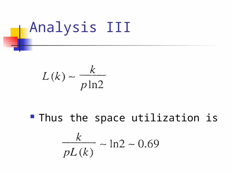
Analysis III

Thus the space utilization is

Overflow pages

To avoid doubling the size of directory, we introduce the idea of overflow pages, i.e., If overflow occurs, than we allocate a

new (overflow) page instead of doubling the directory.

Put the new record into the overflow page, and put the pointer of overflow page to the original page. (like chaining.)

Overflow pages II

Obviously, it will improve the utilization, but increases the retrieval time.

Larson et. al. concluded that the size of overflow page is from p to p/2 if 80% utilization is enough. (p is the size of page.)

Overflow pages III

The better utilization require to monitor Access time Insert time Total space utilization

Fagin et al. conclude that it performed at least as well or better than B-tree, by simulation.

Extendible Hashing: Bibl.

Fagin, R., Nievergelt, J., Pippenger, N., and Strong, H. R. Extendible Hashing - A Fast Access Method for Dynamic Files. ACM Trans. Database System 4, 3(Sept. 1979), 315-344.

Tamminen, M. Extendible Hashing with Overflow. Information Processing Lett. 15, 5(Dec. 1982), 227-232.

Mendelson, H. Analysis of Extendible Hashing. IEEE Trans. on Software Engineering, SE-8, 6(Nov. 1982), 611-619.

Yao, A. C. A Note on the Analysis of Extendible Hashing. Information Processing Letter 11, 2(1980), 84-86.

Directoryless Dynamic Hashing(Linear Hashing)Ref. "Linear Hashing: A new tool for file and database addressing", VLDB 1980. by W. Litwin.

Ref. Larson, “Dynamic Hash Tables,” Communications of the ACM, pages 446–457, April 1988, Volume 31, Number 4.

If we have the contiguous space and large enough, we could estimate the directory and leave the memory management mechanism to OS, e.g., paging.

Figure 8.12

Trie in figure 8.9(a)

Map Trie to the contiguous space without directory.

Linear Hashing II.

Drawback of previous mapping: It wastes space, since we need to double the contiguous space if page overflow occurs.

How to improve: Intuitively, add only one page, and rehash this space!

Ref. Larson, “Dynamic Hash Tables,” Communications of the ACM, pages 446–457, April 1988, Volume 31, Number 4.

Add new page one by one.

Eventually, the space is doubled. Begin new phase!

Linear Hashing II.

The suitable family of hashing functions:

Where N is the minimum size of hash table, c is a constant, and M is a large prime.

This family of hash functions is given by Larson, “Dynamic Hash Tables,” Communications of the ACM, pages 446–457, April 1988, Volume 31, Number 4.

Example

Ref. Larson, “Dynamic Hash Tables,” Communications of the ACM, pages 446–457, April 1988, Volume 31, Number 4.

The case that keys is rehashed into new page.

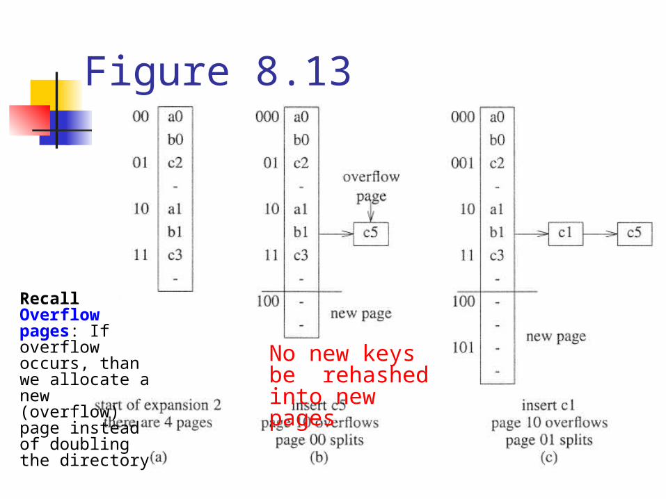
Figure 8.13

Recall Overflow pages: If overflow occurs, than we allocate a new (overflow) page instead of doubling the directory

No new keys be rehashed into new pages

Linear Hashing III.

The family of hash function in the textbook, hash(key, r) := key (mod 2^{r-1})

Analysis

Space utilization is not good! [Litwin] ~ 60% Litwin suggested to keep overflows

until the space utilization exceeds the predefined amount.

Also could be solved by open addressing, etc.