Enhanced Interval Trees for Dynamic IP Router-Tables ∗

Haibin Lu Sartaj Sahni{halu,sahni}@cise.ufl.edu

Department of Computer and Information Science and EngineeringUniversity of Florida, Gainesville, FL 32611

Abstract

We develop an enhanced interval tree data structure that is suitable for the representation ofdynamic IP router tables. Several refinements of this enhanced structure are proposed for a variety ofIP router tables. For example, the data structure called BOB (binary tree on binary tree) is developedfor dynamic router tables in which the rule filters are nonintersecting ranges and in which ties arebroken by selecting the highest-priority rule that matches a destination address. Prefix filters are aspecial case of nonintersecting ranges and the commonly used longest-prefix tie breaker is a specialcase of the highest-priority tie breaker. When an n-rule router table is represented using BOB, thehighest-priority rule that matches a destination address may be found in O(log2 n) time; a new rulemay be inserted and an old one deleted in O(log n) time. For general ranges, the data structure CBOB(compact BOB is proposed). For the case when all rule filters are prefixes, the data structure PBOB(prefix BOB) permits highest-priority matching as well as rule insertion and deletion in O(W ) time,where W is the length of the longest prefix, each. When all rule filters are prefixes and longest-prefixmatching is to be done, the data structures LMPBOB (longest matching-prefix BOB) permits longest-prefix matching in O(W ) time; rule insertion and deletion each take O(log n) time. On practical ruletables, BOB and PBOB perform each of the three dynamic-table operations in O(log n) time andwith O(log n) cache misses. The number of cache misses incurred by LMPBOB is also O(log n).Experimental results also are presented.

Keywords: Interval trees, packet classification, packet routing, router tables, highest-prioritymatching, longest-prefix matching, dynamic rule-tables, rule insertion and deletion.

1 Introduction

An Internet router classifies incoming packets into flows1 utilizing information contained in packet headers

and a table of (classification) rules. This table is called the rule table (equivalently, router table). In this

paper, we assume that packet classification is done using only the destination address of a packet. Each

rule-table rule is a pair of the form (F,A), where F is a filter and A is an action. The action component

of a rule specifies what is to be done when a packet that satisfies the rule filter is received. Sample actions

are drop the packet, forward the packet along a certain output link, and reserve a specified amount of

bandwidth. We also assume that each rule filter is a range [u, v] of destination addresses. A filter matches

∗This work was supported, in part, by the National Science Foundation under grant CCR-9912395.1A flow is a set of packets that are to be treated similarly for routing purposes.

1

the destination address d iff u ≤ d ≤ v. Since an Internet rule-table may contain several rules that match

a given destination address d, a tie breaker is used to select a rule from the set of rules that match

d. For purposes of this tie breaker, each rule is assigned a priority, and the highest-priority rule that

matches d determines the action for all packets whose destination address is d (We may assume either

that all priorities are distinct or that selection among rules that have the same priority may be done in an

arbitrary fashion). Rule tables in which the filters are ranges and in which the highest-priority matching

filter tie breaker is used are referred to as highest-priority range-tables (HPRT). When the filters of no

two rules of an HPRT intersect, the HPRT is a nonintersecting HPRT (NHPRT).

In a static rule table, the rule set does not vary in time. For these tables, we are concerned primarily

with the following metrics:

1. Time required to process an incoming packet. This is the time required to search the rule table for

the rule to use. We refer to this operation as a lookup.

2. Preprocessing time. This is the time to create the rule-table data structure.

3. Storage requirement. That is, how much memory is required by the rule-table data structure?

In practice, rule tables are seldom truly static. At best, rules may be added to or deleted from the

rule table infrequently. Typically, in a “static” rule table, inserts/deletes are batched and the rule-table

data structure reconstructed as needed.

In a dynamic rule table, rules are added/deleted with some frequency and the action component of the

rule may also be changed. For such tables, inserts/deletes are not batched. Rather, they are performed

in real time. For such tables, we are concerned additionally with the time required to insert/delete a rule.

For a dynamic rule table, the initial rule-table data structure is constructed by starting with an empty

data structure and then inserting the initial set of rules into the data structure one by one. So, typically,

in the case of dynamic tables, the preprocessing metric, mentioned above, is very closely related to the

insert time.

Data structures for rule tables in which each filter is a destination address prefix and the rule priority

is the length of this prefix2 have been intensely researched in recent years. We refer to rule tables of this

type as longest-matching prefix-tables (LMPT). Although every LMPT is also an NHPRT, an NHPRT

may not be an LMPT. We use W to denote the maximum possible length of a prefix. In IPv4, W = 32

and in IPv6, W = 128.

2For example, the filter 10* matches all destination addresses that begin with the bit sequence 10; the length of thisprefix is 2.

2

Although much of the research in the router-table area has focused on static prefix-tables, our focus

here is dynamic prefix- and range-tables. We are motivated to study such tables for the following

reasons. First, in a prefix-table, aggregation of prefixes is limited to pairs of prefixes that have the same

length and match contiguous addresses. In a range-table, we may aggregate prefixes and ranges that

match contiguous addresses regardless of the lengths of the prefixes and ranges being aggregated. So,

range aggregation is expected to result in router tables that have fewer rules. Second, with the move to

QoS services, router-table rules include ranges for port numbers (for example). Although ternary content

addressable memories (TCAMs), the most popular hardware solution for prefix tables, can handle prefixes

naturally, they are unable to handle ranges directly. Rather, ranges are decomposed into prefixes. Since

each range takes up to 2W − 2 prefixes to represent, decomposing ranges into prefixes may result in

a large increase in router-table size. Since data structures for multidimensional classifiers are built on

top of data structures for one-dimensional classifiers, it is necessary to develop good data structures

for one-dimensional range router-tables (as we do in this paper). Third, in firewall filter-tables, the

highest-priority matching tie breaker, which is a generalization of the first matching-rule tie breaker, is

usually used. Fourth, dynamic tables that permit high-speed inserts and deletes are essential in QoS

applications [1]. For example, edge routers that do stateful filtering require high-speed updates [2]. For

forwarding tables at backbone routers, Labovitz et al. [3] found that the update rate could reach as

high as 1000 per second. These updates stem from route failures, route repair and route fail-over. With

the number of autonomous systems continuously increasing, it’s reasonable to expect an increase in the

required update rate.

There are basically two strategies to handle router-table updates. In one, we employ two copies–

working and shadow–of the router table. Lookups are done using the working table. Updates are

performed, in the background (either in real time on the shadow table or by batching updates and

reconstructing an updated shadow at suitable intervals); periodically, the shadow replaces the working

table. In this mode of operation, static schemes that optimize lookup time are suitable. However, in

this mode of operation, many packets may be misclassified, because the working copy isn’t immediately

updated. The number of misclassified packets depends on the periodicity with which the working table

can be replaced by an updated shadow. Further, additional memory is required for the shadow table

and/or for periodic reconstruction of the working table. In the second mode of operation, there is

only a working table and updates are made directly to the working table. In this mode, no packet is

improperly classified. However, packet classification may be delayed while a preceding update completes.

3

To minimize this delay, it is essential that updates be done as fast as possible.

In this paper, we focus on data structures for dynamic NHPRTs, HPPTs and LMPTs. The case

of general ranges (i.e., possibly intersecting ranges) is briefly considered in Section 6. We begin, in

Section 3, by developing the terminology used in this paper. In Section 4, we review two popular but

different interval tree structures. One of these is refined to obtain our proposed enhanced interval tree

structure. In Section 5, we develop the data structure binary tree on binary tree (BOB), which, itself,

is a refinement of our proposed enhanced interval tree structure. This data structure is proposed for the

representation of dynamic NHPRTs. Using BOB, a lookup takes O(log2 n) time and cache misses; a new

rule may be inserted and an old one deleted in O(log n) time and cache misses. For HPPTs, we propose

a modified version of BOB–PBOB (prefix BOB)–in Section 7. Using PBOB, a lookup, rule insertion and

deletion each take O(W ) time and cache misses. In Section 8, we develop the data structures LMPBOB

(longest matching-prefix BOB) for LMPTs. Using LMPBOB, the longest matching-prefix may be found

in O(W ) time and O(log n) cache misses; rule insertion and deletion each take O(log n) time and cache

misses. On practical rule tables, BOB and PBOB perform each of the three dynamic-table operations

in O(log n) time and with O(log n) cache misses. Note that since an LMPT is also an HPPT and an

NPHRT, BOB and PBOB may be used for LMPTs also. Experimental results are presented in Section 9.

2 Related Work

Data structures for longest-matching prefix-tables (LMPT) have been intensely researched in recent

years. Ruiz-Sanchez et al. [4] review data structures for static LMPTs and Sahni et al. [5] review data

structures for both static and dynamic LMPTs.

Ternary content-addressible memories, TCAMs, use parallelism to achieve O(1) lookup [6]. A prefix

may be inserted or deleted in O(W ) time, where W is the length of the longest prefix [7]3. Although

TCAMs provide a simple and efficient solution for static and dynamic router tables, this solution re-

quires special hardware, costs more, and uses more power and board space than solutions that employ

SDRAMs [8]. EZchip Technologies, for example, claim that classifiers can forgo TCAMs in favor of

commodity memory solutions [2,8]. Algorithmic approaches that have lower power consumption and are

conservative on board space at the price of slightly increased search latency are sought. “System vendors

are willing to accept some latency in their searches if it means lowering the power of a line card” [8].

Several trie-based data structures for LMPTs have been proposed [9–15]. Structures such as that of [9]

3More precisely, W may be defined to be the number of different prefix lengths in the table.

4

perform each of the dynamic router-table operations (lookup, insert, delete) in O(W ) time. Others (e.g.,

[10–16]) attempt to optimize lookup time and memory requirement through an expensive preprocessing

step. These structures, while providing very fast lookup capability, have a prohibitive insert/delete time

and so, they are suitable only for static router-tables (i.e., tables into/from which no inserts and deletes

take place).

Gupta et al. [16], for example, propose the DIR-24-8 scheme. This scheme uses a 32 MB table with

224 16-bit entries together with a potentially much larger table that has t 256-entry blocks, where t is

the number of distinct 24-bit sequences x such x is the first 24 bits of some length 25 or greater prefix

of the router table. Using these two tables, it is possible to find the longest matching-prefix in at most 2

memory accesses. Although the scheme using an excessive amount of memory, Gupta et al. [16] propose

alternatives that use less memory but require more memory accesses.

Waldvogel et al. [17] have proposed a scheme that performs a binary search on hash tables organized

by prefix length. This binary search scheme has an expected complexity of O(log W ) for lookup. An

alternative adaptation of binary search to longest-prefix matching is developed in [18]. Using this adap-

tation, a lookup in a table that has n prefixes takes O(W + log n) = O(W ) time. Because the schemes

of [17] and [18] use expensive precomputation, they are not suited for a dynamic router-tables.

For dynamic TCAM tables, Shah and Gupta [7] show how to insert and delete in O(W ) time. Con-

tinuing with the special-purpose hardware theme, Basu et al. [19] describe a dynamic router-table design

for pipelined forwarding engines.

Suri et al. [20] have proposed an all-algorithmic design for dynamic LMPTs. Their design employs the

B-tree data structure and permits one to find the longest matching-prefix, LMP (d), in O(log n) time.

However, inserts/deletes take O(W log n) time. When W bits fit in O(1) words (as is the case for IPv4

and IPv6 prefixes) logical operations on W -bit vectors can be done in O(1) time each. In this case, the

scheme of [20] takes O(W + log n) = O(W ) time for an update. The number of cache misses that occur

when the data structure of [20] is used is O(log n) per operation.

Sahni and Kim [21, 22] develop data structures, called a collection of red-black trees (CRBT) and

alternative collection of red-black trees (ACRBT), that support the three operations of a dynamic LMPT

in O(log n) time each. The number of cache misses is also O(log n). In [22], Sahni and Kim show that

their ACRBT structure is easily modified to extend the biased-skip-list structure of Ergun et al. [23]

so as to obtain a biased-skip-list structure for dynamic LMPTs. Using this modified biased skip-list

structure, lookup, insert, and delete can each be done in O(log n) expected time and O(log n) expected

5

cache misses. Like the original biased-skip list structure of [23], the modified structure of [22] adapts

so as to perform lookups faster for bursty access patterns than for non-bursty patterns. The ACRBT

structure may also be adapted to obtain a collection of splay trees structure [22], which performs the

three dynamic LMPT operations in O(log n) amortized time and which adapts to provide faster lookups

for bursty traffic. Lu and Sahni [24] show how priority search trees may be used to support the three

dynamic router-table operations in O(log n) time each. Their work applies to both prefix filters as well

as to the case of a set of conflict-free range filters.

When highest-priority prefix-table (HPPT) is represented as a binary trie [25], each of the three

operations takes O(W ) time and cache misses. Gupta and McKeown [26] have developed two data

structures for dynamic highest-priority range-table (HPRT)—heap on trie (HOT) and binary search tree

on trie (BOT). The HOT structure takes O(W ) time for a lookup and O(W log n) time for an insert or

delete. The BOT structure takes O(W log n) time for a lookup and O(W ) time for an insert/delete. The

number of cache misses in a HOT and BOT is asymptotically the same as the time complexity of the

corresponding operation.

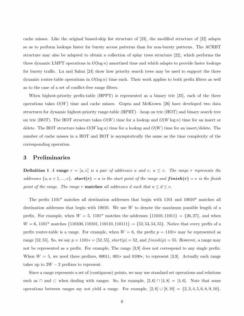
3 Preliminaries

Definition 1 A range r = [u, v] is a pair of addresses u and v, u ≤ v. The range r represents the

addresses {u, u + 1, ..., v}. start(r) = u is the start point of the range and finish(r) = v is the finish

point of the range. The range r matches all addresses d such that u ≤ d ≤ v.

The prefix 1101* matches all destination addresses that begin with 1101 and 10010* matches all

destination addresses that begin with 10010. We use W to denote the maximum possible length of a

prefix. For example, when W = 5, 1101* matches the addresses {11010, 11011} = {26, 27}, and when

W = 6, 1101* matches {110100, 110101, 110110, 110111} = {52, 53, 54, 55}. Notice that every prefix of a

prefix router-table is a range. For example, when W = 6, the prefix p = 1101∗ may be represented as

range [52, 55]. So, we say p = 1101∗ = [52, 55], start(p) = 52, and finish(p) = 55. However, a range may

not be represented as a prefix. For example, The range [3,9] does not correspond to any single prefix.

When W = 5, we need three prefixes, 00011, 001∗ and 0100∗, to represent [3,9]. Actually each range

takes up to 2W − 2 prefixes to represent.

Since a range represents a set of (contiguous) points, we may use standard set operations and relations

such as ∩ and ⊂ when dealing with ranges. So, for example, [2, 6] ∩ [4, 8] = [4, 6]. Note that some

operations between ranges my not yield a range. For example, [2, 6] ∪ [8, 10] = {2, 3, 4, 5, 6, 8, 9, 10},

6

u v x yx y u v

(a)

u vx yx yu v

(b)

u vx yx yu v(c)

Figure 1: Relationships between pairs of ranges. (a). Disjoint ranges. (b). Nested ranges. (c). Inter-secting ranges.

which is not a range.

Definition 2 Let r = [u, v] and s = [x, y] be two ranges.

(a) r and s are disjoint iff r ∩ s = ∅

(b) r and s are nested iff one of the ranges is contained within the other, i.e., r ⊆ s or s ⊆ r

(c) r and s are intersecting iff r and s have a nonempty intersection that is different from both r and

s, i.e., u < x ≤ v < y or x < u ≤ y < v.

Figure 1 shows the relationships between pairs of ranges. [2, 4] and [6, 9] are disjoint; [2,4] and [3,4]

are nested; [2,4] and [4,6] intersect.

Definition 3 Let R be a range set. ranges(d, R) (or simply ranges(d) when R is implicit) is the

subset of ranges of R that match the destination address d.

When R = {[2, 4], [1, 6], [7, 10]}, ranges(3) = {[2, 4], [1, 6]}.

4 Enhanced Interval Tree

4.1 Interval Trees

Two fundamentally different interval tree data structures for range data are described in [27] and [28].

Although both employ a red-black tree and in both each range is stored in exactly one node of this

red-black tree, the structures differ in the strategy used to allocate ranges to nodes. In the interval tree

data structure of [27], each node of the red-black tree z stores exactly one range, range(z). Hence, the

7

red-black tree has exactly n nodes, where n is the number of ranges. Additionally, each node z stores a

value maxFinish(z), which is the maximum of the finish points of all ranges stored in the subtree rooted

at z. Each range r in the left subtree of z satisfies

(start(r) < start(range(z)) or (start(r) = start(range(z)) and finish(r) > finish(range(z)))

Each range r in the right subtree of z satisfies

(start(r) > start(range(z)) or (start(r) = start(range(z)) and finish(r) < finish(range(z)))

When the prefixes of a router table are stored in the interval tree of [27], prefix insertion and deletion

take O(log n) time. However, it takes O(min{n, k log n}) time to find the longest matching-prefix (as

well as the highest-priority matching-prefix), where k is the number of prefixes that match the given

destination address.

In the interval tree of [28], each node z of the red-black tree stores a non-empty subset, ranges(z)4,

of the ranges. Hence the number of nodes in the red-black tree is O(n). There is a point, point(z),

associated with every node of the red-black tree. The points in the left subtree of z are < point(z) and

those in its right subtree are > point(z). Hence, we call this red-black tree the point search tree (PTST).

Let R be the set of ranges stored in the PTST and let root be the root of the PTST. All ranges r ∈ R

such that start(r) ≤ point(z) ≤ finish(r) are stored in the root (these ranges define ranges(z)); all

r ∈ R such that finish(r) < point(z) are stored in the left subtree of z; and the remaining ranges of

R are stored in the right subtree of z. This range allocation rule is recursively applied to the left and

right subtrees of the PTST. In each node z of the PTST, two lists, left(z) and right(z), are maintained.

left(z) stores the ranges of ranges(z) sorted by their start points while right(z) stores these ranges

sorted by their finish points. Using this interval tree organization for a prefix router-table, the longest

matching-prefix (as well as the highest-priority matching-prefix) can be found in O(log n+k) time. Prefix

insertion and deletion are very expensive.

The high complexity of the update operations stems from the requirement that ranges(z) be non-

empty for every node z. Consider the deletion operation. Suppose that following the deletion of a range,

ranges(v) becomes empty for some node v. When v is a degree-2 node, we replace point(v) with either

the largest point in the left subtree of v or the smallest point in the right subtree of v. Suppose we do

the former. Further suppose that the largest point is in the node y. The ranges stored in all nodes on

4We have overloaded the function ranges. When u is a node, ranges(u) refers to the ranges stored in node u; when u isa destination address, ranges(u) refers to the ranges that match u

8

(a) (b) (c)

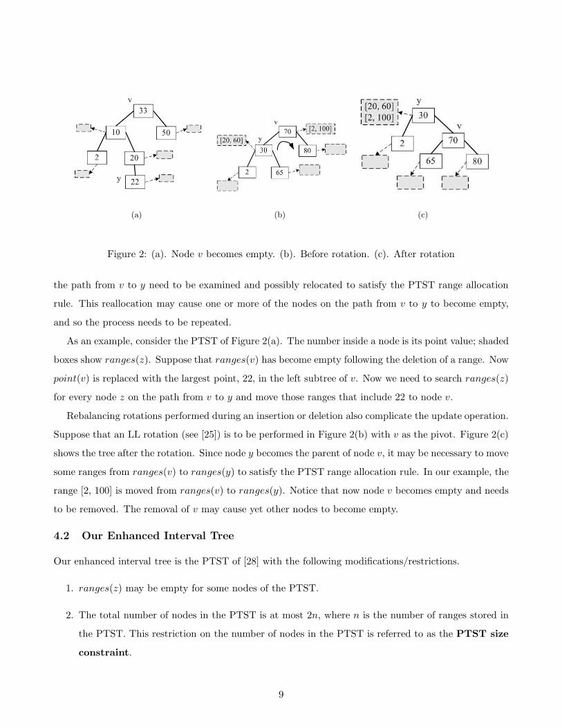
Figure 2: (a). Node v becomes empty. (b). Before rotation. (c). After rotation

the path from v to y need to be examined and possibly relocated to satisfy the PTST range allocation

rule. This reallocation may cause one or more of the nodes on the path from v to y to become empty,

and so the process needs to be repeated.

As an example, consider the PTST of Figure 2(a). The number inside a node is its point value; shaded

boxes show ranges(z). Suppose that ranges(v) has become empty following the deletion of a range. Now

point(v) is replaced with the largest point, 22, in the left subtree of v. Now we need to search ranges(z)

for every node z on the path from v to y and move those ranges that include 22 to node v.

Rebalancing rotations performed during an insertion or deletion also complicate the update operation.

Suppose that an LL rotation (see [25]) is to be performed in Figure 2(b) with v as the pivot. Figure 2(c)

shows the tree after the rotation. Since node y becomes the parent of node v, it may be necessary to move

some ranges from ranges(v) to ranges(y) to satisfy the PTST range allocation rule. In our example, the

range [2, 100] is moved from ranges(v) to ranges(y). Notice that now node v becomes empty and needs

to be removed. The removal of v may cause yet other nodes to become empty.

4.2 Our Enhanced Interval Tree

Our enhanced interval tree is the PTST of [28] with the following modifications/restrictions.

1. ranges(z) may be empty for some nodes of the PTST.

2. The total number of nodes in the PTST is at most 2n, where n is the number of ranges stored in

the PTST. This restriction on the number of nodes in the PTST is referred to as the PTST size

constraint.

9

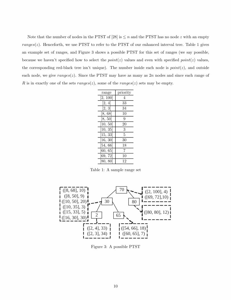
Note that the number of nodes in the PTST of [28] is ≤ n and the PTST has no node z with an empty

ranges(z). Henceforth, we use PTST to refer to the PTST of our enhanced interval tree. Table 1 gives

an example set of ranges, and Figure 3 shows a possible PTST for this set of ranges (we say possible,

because we haven’t specified how to select the point(z) values and even with specified point(z) values,

the corresponding red-black tree isn’t unique). The number inside each node is point(z), and outside

each node, we give ranges(z). Since the PTST may have as many as 2n nodes and since each range of

R is in exactly one of the sets ranges(z), some of the ranges(z) sets may be empty.

range priority

[2, 100] 4

[2, 4] 33

[2, 3] 34

[8, 68] 10

[8, 50] 9

[10, 50] 20

[10, 35] 3

[15, 33] 5

[16, 30] 30

[54, 66] 18

[60, 65] 7

[69, 72] 10

[80, 80] 12

Table 1: A sample range set

70

30 80

2 65

([2, 100], 4) ([69, 72],10)

([80, 80], 12)

([54, 66], 18) ([60, 65], 7)

([8, 68], 10) ([8, 50], 9)

([10, 50], 20) ([10, 35], 3) ([15, 33], 5) ([16, 30], 30)

([2, 4], 33) ([2, 3], 34)

Figure 3: A possible PTST

10

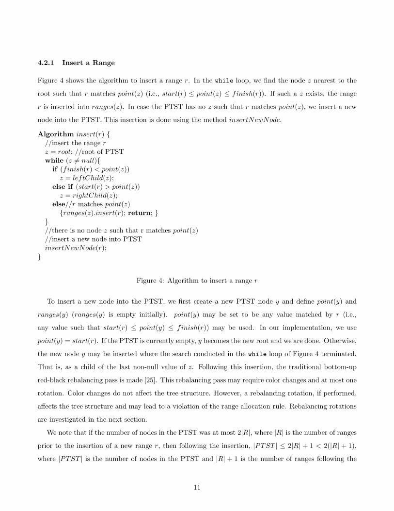
4.2.1 Insert a Range

Figure 4 shows the algorithm to insert a range r. In the while loop, we find the node z nearest to the

root such that r matches point(z) (i.e., start(r) ≤ point(z) ≤ finish(r)). If such a z exists, the range

r is inserted into ranges(z). In case the PTST has no z such that r matches point(z), we insert a new

node into the PTST. This insertion is done using the method insertNewNode.

Algorithm insert(r) {//insert the range r

z = root; //root of PTSTwhile (z 6= null){

if (finish(r) < point(z))z = leftChild(z);

else if (start(r) > point(z))z = rightChild(z);

else//r matches point(z){ranges(z).insert(r); return; }

}//there is no node z such that r matches point(z)//insert a new node into PTSTinsertNewNode(r);

}

Figure 4: Algorithm to insert a range r

To insert a new node into the PTST, we first create a new PTST node y and define point(y) and

ranges(y) (ranges(y) is empty initially). point(y) may be set to be any value matched by r (i.e.,

any value such that start(r) ≤ point(y) ≤ finish(r)) may be used. In our implementation, we use

point(y) = start(r). If the PTST is currently empty, y becomes the new root and we are done. Otherwise,

the new node y may be inserted where the search conducted in the while loop of Figure 4 terminated.

That is, as a child of the last non-null value of z. Following this insertion, the traditional bottom-up

red-black rebalancing pass is made [25]. This rebalancing pass may require color changes and at most one

rotation. Color changes do not affect the tree structure. However, a rebalancing rotation, if performed,

affects the tree structure and may lead to a violation of the range allocation rule. Rebalancing rotations

are investigated in the next section.

We note that if the number of nodes in the PTST was at most 2|R|, where |R| is the number of ranges

prior to the insertion of a new range r, then following the insertion, |PTST | ≤ 2|R| + 1 < 2(|R| + 1),

where |PTST | is the number of nodes in the PTST and |R| + 1 is the number of ranges following the

11

insertion of r. Hence an insert does not violate the PTST size constraint.

Exclusive of the time required to perform the tasks associated with a rebalancing rotation (notice

that at most one rebalancing rotation is needed following an insert), the time required to insert a range

is O(height(PTST )) = O(log n).

4.2.2 Red-Black-Tree Rotations

Figures 5 and 6, respectively, show the red-black LL and RR rotations used to rebalance a red-black

tree following an insert or delete (see [25]). In these figures, pt() is an abbreviation for point(). Since

the remaining rotation types, LR and RL, may, respectively, be viewed as a RR rotation followed by an

LL rotation and an LL rotation followed by an RR rotation, it suffices to examine LL and RR rotations

alone.

pt ( x )

pt (y )

a b

c LL

pt (y )

pt ( x ) a

b c

y

x y

x

Figure 5: LL Rotation

pt (y )

pt ( x )

a b

c RR

pt ( x )

pt (y ) a

b c

x

y x

y

Figure 6: RR Rotation

Lemma 1 Let R be a set of ranges. Let ranges(z) ⊆ R be the ranges allocated by the range allocation

rule to node z of the PTST prior to an LL or RR rotation. Let ranges′(z) be this subset for the PTST

node z following the rotation. Then ranges(z) = ranges′(z) for all nodes z in the subtrees a, b, and c of

12

Figures 5 and 6.

Proof Consider an LL rotation. Let ranges(subtree(x)) be the union of the range sets allocated to the

nodes in the subtree whose root is x. Since the range allocation rule allocates each range r to the node

z nearest the root such that r matches point(z), ranges(subtree(x)) = ranges′(subtree(y)). Further,

r ∈ ranges(a) iff r ∈ ranges(subtree(x)) and finish(r) < point(y). Consequently, r ∈ ranges′(a). From

this and the fact that the LL rotation doesn’t change the positioning of nodes in a, it follows that for

every node z in the subtree a, ranges(a) = ranges′(a). The proof for the nodes in b and c as well as for

the RR rotation is similar.

Let x and y be as in Figures 5 and 6. From Lemma 1, it follows that ranges(z) = ranges′(z) for all z

in the PTST except possibly for z ∈ {x, y}. It is not too difficult to see that ranges′(y) = ranges(y)∪S

and ranges′(x) = ranges(x) − S, where S = {r|r ∈ ranges(x) and start(r) ≤ point(y) ≤ finish(r)}.

The time required to do an LL or RR rotation depends on the time taken to determine S, remove S

from ranges(x), and add S to ranges(y). This depends on the data structure used to represent ranges().

The time for LR and RL rotations is roughly twice that for LL and RR rotations.

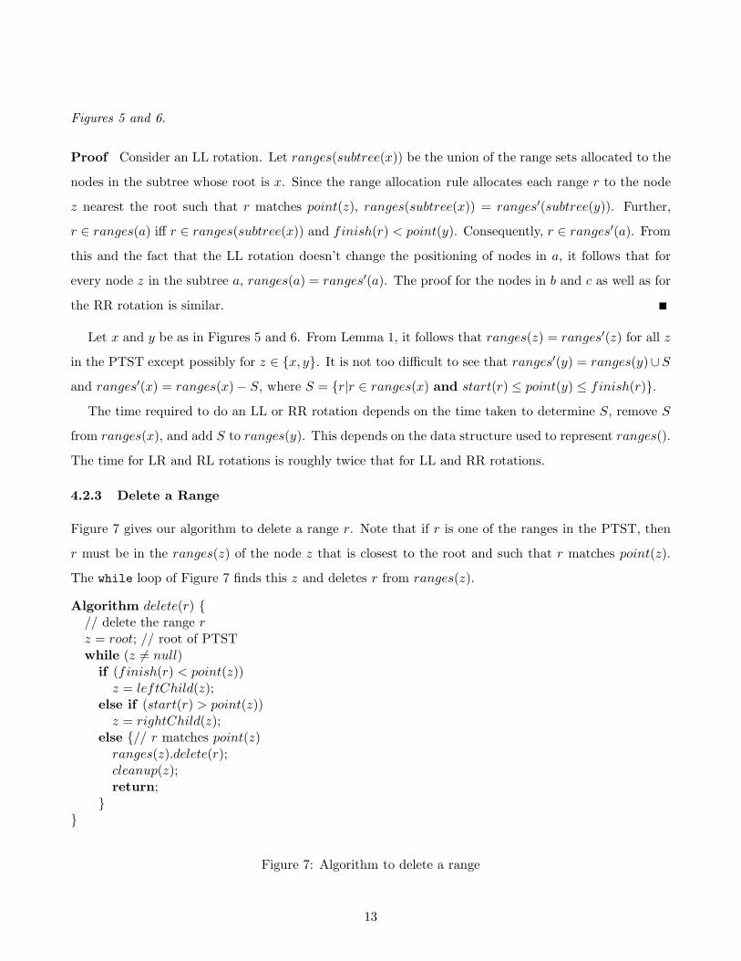
4.2.3 Delete a Range

Figure 7 gives our algorithm to delete a range r. Note that if r is one of the ranges in the PTST, then

r must be in the ranges(z) of the node z that is closest to the root and such that r matches point(z).

The while loop of Figure 7 finds this z and deletes r from ranges(z).

Algorithm delete(r) {// delete the range r

z = root; // root of PTSTwhile (z 6= null)

if (finish(r) < point(z))z = leftChild(z);

else if (start(r) > point(z))z = rightChild(z);

else {// r matches point(z)ranges(z).delete(r);cleanup(z);return;

}}

Figure 7: Algorithm to delete a range

13

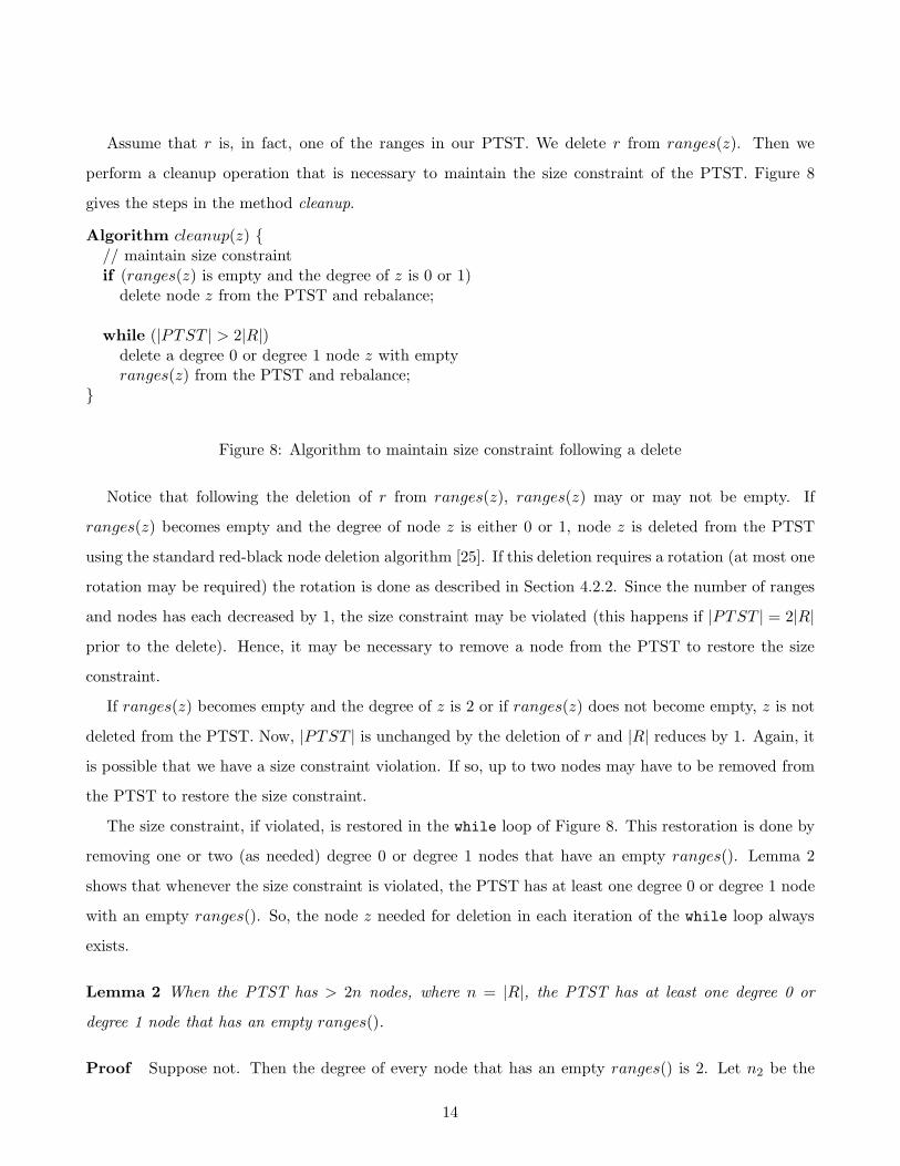
Assume that r is, in fact, one of the ranges in our PTST. We delete r from ranges(z). Then we

perform a cleanup operation that is necessary to maintain the size constraint of the PTST. Figure 8

gives the steps in the method cleanup.

Algorithm cleanup(z) {// maintain size constraintif (ranges(z) is empty and the degree of z is 0 or 1)

delete node z from the PTST and rebalance;

while (|PTST | > 2|R|)delete a degree 0 or degree 1 node z with emptyranges(z) from the PTST and rebalance;

}

Figure 8: Algorithm to maintain size constraint following a delete

Notice that following the deletion of r from ranges(z), ranges(z) may or may not be empty. If

ranges(z) becomes empty and the degree of node z is either 0 or 1, node z is deleted from the PTST

using the standard red-black node deletion algorithm [25]. If this deletion requires a rotation (at most one

rotation may be required) the rotation is done as described in Section 4.2.2. Since the number of ranges

and nodes has each decreased by 1, the size constraint may be violated (this happens if |PTST | = 2|R|

prior to the delete). Hence, it may be necessary to remove a node from the PTST to restore the size

constraint.

If ranges(z) becomes empty and the degree of z is 2 or if ranges(z) does not become empty, z is not

deleted from the PTST. Now, |PTST | is unchanged by the deletion of r and |R| reduces by 1. Again, it

is possible that we have a size constraint violation. If so, up to two nodes may have to be removed from

the PTST to restore the size constraint.

The size constraint, if violated, is restored in the while loop of Figure 8. This restoration is done by

removing one or two (as needed) degree 0 or degree 1 nodes that have an empty ranges(). Lemma 2

shows that whenever the size constraint is violated, the PTST has at least one degree 0 or degree 1 node

with an empty ranges(). So, the node z needed for deletion in each iteration of the while loop always

exists.

Lemma 2 When the PTST has > 2n nodes, where n = |R|, the PTST has at least one degree 0 or

degree 1 node that has an empty ranges().

Proof Suppose not. Then the degree of every node that has an empty ranges() is 2. Let n2 be the

14

total number of degree 2 nodes, n1 the total number of degree 1 nodes, n0 the total number of degree

0 nodes, ne the total number of nodes that have an empty ranges(), and nn the total number of nodes

that have a nonempty ranges(). Since all PTST nodes that have an empty ranges() are degree 2 nodes,

n2 ≥ ne. Further, since there are only n ranges and each range is stored in exactly one ranges(), there

are at most n nodes that have a nonempty ranges(), i.e., n ≥ nn. Thus n2 + n ≥ ne + nn = |PTST |,

i.e., n2 ≥ |PTST | − n. From [25] (Lemma 5.3), we know that n0 = n2 + 1. Hence, n0 + n1 + n2 =

n2 + 1 + n1 + n2 > n2 + n2 ≥ 2|PTST | − 2n > |PTST |. This contradicts n0 + n1 + n2 = |PTST |.

To find the degree 0 and degree 1 nodes that have an empty ranges() efficiently, we maintain a doubly-

linked list of these nodes. Also, a doubly-linked list of degree 2 nodes that have an empty ranges() is

maintained. When a range is inserted or deleted, PTST nodes may be added/removed from these doubly-

linked lists and nodes may move from one list to another. The required operations can be done in O(1)

time each.

Notice that we only remove degree 0 or degree 1 nodes from the PTST. The cleanup step removes

up to 2 nodes from the PTST. At most one rebalancing rotation is needed following the removal of a

node from the PTST. Thus O(1) number of ranges()s need to be adjusted. The overall delete time is

the O(log n) time needed to find the PTST node z that contains the range r that is to be deleted, plus

the time to delete r from ranges(z), plus the time needed to adjust O(1) number of ranges()s. The

complexity of deleting r from ranges(z) and adjusting ranges()s depends on the data structure used for

ranges()s.

5 BOB for Nonintersecting Ranges

In this section, we refine the enhanced interval tree structure of Section 4.2 to obtain a data structure,

BOB (binary tree on binary tree), for nonintersecting ranges. BOB comprises a red-black PTST as in

Section 4.2. This tree is called the top-level tree. For every node z of the PTST, ranges(z) is represented

as a balanced binary search tree called the range search tree (RST). The RST in each node is called a

second-level tree. Using BOB, we can find the highest-priority matching range in O((log n)(log maxR))

time, where n is the number of ranges and maxR is the maximum number of ranges that match any

destination address (so |ranges(z)| ≤ maxR for every node z of the PTST). Inserting or deleting a range

can be done in O(log n) time. The data structure uses O(n) space.

Sahni and Kim [21] have analyzed the prefixes in several real IPv4 prefix router-tables. They report

that a destination address is matched, on average, by about 1 prefix; the maximum number of prefixes

15

that match a destination address is at most 6. Assuming that this analysis holds true even for real range

router-tables (no data is available for us to perform such an analysis), we conclude that maxR ≤ 6. So,

the expected complexity of BOB on real router-tables is O(log n) per operation. Note that every prefix

set is a set of nonintersecting ranges.

5.1 Nonintersecting Ranges

Definition 4 The range set R is nonintersecting iff no pair of ranges intersect (Figure 1(c)).

Definition 5 Let R be a range set. hpr(d) is the highest-priority range in ranges(d). We assume that

ranges are assigned priorities in such a way that hpr(d) is uniquely defined for every d.

Now we define the < relation between two ranges. Range r is less than range s iff the start point of r

is smaller than the start point of s, or the finish point of r is larger than the finish point of s when they

have the same start point. Note that for every pair, r and s, of different ranges, either r < s or s < r.

Definition 6 Let r and s be two ranges. r < s ⇔

start(r) < start(s) or (start(r) = start(s) and finish(r) > finish(s)).

Lemma 3 Let R be a nonintersecting range set. If r ∩ s 6= ∅ for r , s ∈ R, then the following are true:

1. start(r) < start(s) ⇒ finish(r) ≥ finish(s).

2. finish(r) > finish(s) ⇒ start(r) ≤ start(s).

Proof Straightforward.

5.2 The Data Structure for ranges()

The set of ranges in Table 1 is a nonintersecting range set. For such range set, the ranges in ranges(z) may

be ordered using the < relation of Definition 6. Using this < relation, we put the ranges of ranges(z)

into a red-black tree (any balanced binary search tree structure that supports efficient search, insert,

delete, join, and split may be used) called the range search-tree or RST (z). Each node x of RST (z)

stores exactly one range of ranges(z). We refer to this range as range(x). Every node y in the left

(right) subtree of node x of RST (z) has range(y) < range(x) (range(y) > range(x)). In addition, each

node x stores the quantity mp(x), which is the maximum of the priorities of the ranges associated with

the nodes in the subtree rooted at x. mp(x) may be defined recursively as below.

mp(x) =

{

p(x) if x is leafmax {mp(leftChild(x)),mp(rightChild(x)), p(x)} otherwise

16

where p(x) = priority(range(x)). Figure 9 gives a possible RST structure for ranges(node30) of Figure 3.

[10, 35], 3, 30

[8, 50], 9, 20 [15, 33], 5, 30

[8, 68], 10, 10 [10, 50], 20, 20 [16, 30], 30, 30

Figure 9: An example RST for ranges(node30) of Figure 3. Each node shows (range(x), p(x),mp(x))

Lemma 4 Let z be a node in a PTST and let x be a node in RST (z). Let st(x) = start(range(x)) and

fn(x) = finish(range(x)).

1. For every node y in the right subtree of x, st(y) ≥ st(x) and fn(y) ≤ fn(x).

2. For every node y in the left subtree of x, st(y) ≤ st(x) and fn(y) ≥ fn(x).

Proof For 1, we see that when y is in the right subtree of x, range(y) > range(x). From Definition 6, it

follows that st(y) ≥ st(x). Further, since range(y) ∩ range(x) 6= ∅, if st(y) > st(x), then fn(y) ≤ fn(x)

(Lemma 3); if st(y) = st(x), fn(y) < fn(x) (Definition 6). The proof for 2 is similar.

5.3 Search for hpr(d)

The highest-priority range that matches the destination address d may be found by following a path

from the root of the PTST toward a leaf of the PTST. Figure 10 gives the algorithm. For simplicity, this

algorithm finds hp = priority(hpr(d)) rather than hpr(d). The algorithm is easily modified to return

hpr(d) instead.

We begin by initializing hp = −1 and z is set to the root of the PTST. This initialization assumes

that all priorities are ≥ 0. The variable z is used to follow a path from the root toward a leaf. When

d > point(z), d may be matched only by ranges in RST (z) and those in the right subtree of z. The

method RST(z).hpRight(d,hp) (Figure 11) updates hp to reflect any matching ranges in RST (z). This

method makes use of the fact that d > point(z). Consider a node x of RST (z). If d > fn(x), then d is to

the right (i.e., d > finish(range(x))) of range(x) and also to the right of all ranges in the right subtree

of x. Hence, we may proceed to examine the ranges in the left subtree of x. When d ≤ fn(x), range(x)

17

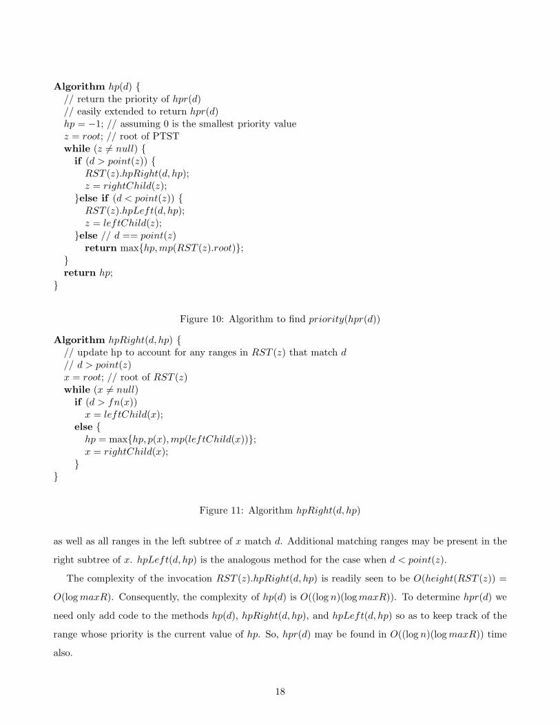
Algorithm hp(d) {// return the priority of hpr(d)// easily extended to return hpr(d)hp = −1; // assuming 0 is the smallest priority valuez = root; // root of PTSTwhile (z 6= null) {

if (d > point(z)) {RST (z).hpRight(d, hp);z = rightChild(z);

}else if (d < point(z)) {RST (z).hpLeft(d, hp);z = leftChild(z);

}else // d == point(z)return max{hp,mp(RST (z).root)};

}return hp;

}

Figure 10: Algorithm to find priority(hpr(d))

Algorithm hpRight(d, hp) {// update hp to account for any ranges in RST (z) that match d

// d > point(z)x = root; // root of RST (z)while (x 6= null)

if (d > fn(x))x = leftChild(x);

else {hp = max{hp, p(x),mp(leftChild(x))};x = rightChild(x);

}}

Figure 11: Algorithm hpRight(d, hp)

as well as all ranges in the left subtree of x match d. Additional matching ranges may be present in the

right subtree of x. hpLeft(d, hp) is the analogous method for the case when d < point(z).

The complexity of the invocation RST (z).hpRight(d, hp) is readily seen to be O(height(RST (z)) =

O(log maxR). Consequently, the complexity of hp(d) is O((log n)(log maxR)). To determine hpr(d) we

need only add code to the methods hp(d), hpRight(d, hp), and hpLeft(d, hp) so as to keep track of the

range whose priority is the current value of hp. So, hpr(d) may be found in O((log n)(log maxR)) time

also.

18

5.4 Adjust RST ()s During Red-Black-Tree Rotations

Since we are dealing with a set of nonintersecting ranges, all ranges in ranges(y) are nested within the

ranges of S (see Section 4.2.2). Figure 12 shows the ranges of ranges(x) using solid lines and those of

ranges(y) using broken lines. S is the set of ranges drawn above ranges(y) (i.e., the solid lines above

the broken lines).

pt ( y ) pt ( x ) pt ( x ) pt ( y )

msr ( pt ( y ), ranges ( x )) msr ( pt ( y ), ranges ( x ))

LL RR

Figure 12: ranges(x) and ranges(y) for LL and RR rotations. Nodes x and y are as in Figures 5 and 6

The range rMax of S with largest start() value may be found by searching RST (x) for the range

with largest start() value that matches point(y). (Note that rMax = msr(point(y), ranges(x)).) Since

RST (x) is a binary search tree of an ordered set of ranges (Definition 6), rMax may be found in

O(height(RST (x)) time by following a path from the root downward. If rMax doesn’t exist, S = ∅,

ranges′(x) = ranges(x) and ranges′(y) = ranges(y).

Assume that rMax exists. We may use the split operation [25] to extract from RST (x) the ranges

that belong to S. The operation

RST (x) → split(small, rMax, big)

separates RST (x) into an RST small of ranges < (Definition 6) than rMax and an RST big of ranges

> than rMax. We see that RST ′(x) = big and RST ′(y) = join(small, rMax,RST (y)), where join [25]

combines the red-black tree small with ranges < rMax, the range rMax, and the red-black tree RST (y)

with ranges > rMax into a single red-black tree.

The standard split and join operations of [25] need to be modified slightly so as to update the mp

values of affected nodes. This modification doesn’t affect the asymptotic complexity, which is logarithmic

19

in the number of nodes in the tree being split or logarithmic in the sum of the number of nodes in the

two trees being joined, of the split and join operations. So, the complexity of performing an LL or RR

rotation (and hence of performing an LR or RL rotation) in the PTST is O(log maxR).

5.5 Insert/Delete a Range

A range r that is known to have no intersection with any of the existing ranges in the router table, may

be inserted using the algorithm of Figure 4. When a new PTST node y is created, RST (y) has only a

root node and this root contains r; its mp value is priority(r).

A rebalancing rotation can be done in O(log maxR) time. Since at most one rebalancing rotation

is needed following an insert, the time to insert a range is O(log n + log maxR) = O(log n). In case it

is necessary for us to verify that the range to be inserted does not intersect an existing range, we can

augment the PTST with priority search trees as in [24] and use these trees for intersection detection.

The overall complexity of an insert remains O(log n).

Assume that r is, in fact, one of the ranges RST (z) of our PTST node z. To delete r from RST (z),

we use the standard red-black deletion algorithm [25] modified to update mp values as necessary.

It takes O(log n) time to find the PTST node z that contains the range r that is to be deleted. Another

O(log maxR) time is needed to delete r from RST (z). The cleanup step removes up to 2 nodes from the

PTST. This takes another O(log n + log maxR) time. So, the overall delete time is O(log n).

6 Compact BOB (CBOB) for General Range-Tables

In this section, we deal with general ranges that may intersect. We assume that maxR, the maximum

number of ranges that match any destination address is a small constant. Hence, |ranges(z)| is small for

every node z of the PTST. Because of this assumption, it suffices to use an array linear list (ALL, [29])

to represent ranges(z). In each node z of CBOB, we maintain 2 ALLs. ALLleft(z) comprises pairs of

the form (range, priority) sorted by the start points of the ranges in ranges(z). ALLright(z) comprises

pairs of the form (range, priority) sorted by the finish points of the ranges in ranges(z). Notice that

these two lists are the same as the two lists stored in each node of the interval tree of [28].

Figure 13 gives the algorithm to find the priority of the highest-priority range that matches the destina-

tion address d. The method ALLleft(z).maxp() returns the highest priority of any range in ALLleft(z)

(note that all ranges in ALLleft(z) match point(z)). The method ALLleft(z).searchALL(d, hp) exam-

ines the ranges in ALLleft(z) and updates hp taking into account the priorities of those ranges that

20

match d.

Algorithm hp(d) {// return the priority of hpp(d)// easily extended to return hpp(d)hp = −1; // assuming 0 is the smallest priority valuez = root; // root of PTSTwhile (z 6= null) {

if (d == point(z))return max{hp,ALLleft(z).maxp()};

if (d < point(z)){ALLleft(z).searchALL(d, hp);z = leftChild(z);

}else{

ALLright(z).searchALL(d, hp);z = rightChild(z);

}}return hp;

}

Figure 13: Algorithm to find priority(hpp(d))

The number of PTST nodes reached in the while loop of Figure 13 is O(log n) and the time spent

at each node z that is reached is |ranges(z)| ≤ maxR. So, the complexity of our lookup algorithm

is O(log n + maxR). The CBOB algorithms to insert/delete a range follow the strategy described in

Section 4.2 for an enhanced interval tree. Since adjusting ranges(), following a rotation, takes O(maxR)

for an array linear list, the CBOB algorithms to insert/delete a range take O(log n + maxR) time. As

noted earlier, maxR is a small constant; so, in practice, CBOB takes O(log n) time and makes this many

cache misses per operation (lookup, insert and delete).

7 Highest-Priority Prefix-Tables (HPPTs)—PBOB

7.1 The Data Structure

When all rule filters are prefixes, maxR ≤ min{n,W}. Hence, if BOB is used to represent an HPPT, the

search complexity is O(log n ∗ min{log n, log W}); the insert and delete complexities are O(log n) each.

Since maxR ≤ 6 for real prefix router-tables, we may expect to see better performance using a

simpler structure (i.e., a structure with smaller overhead and possibly worse asymptotic complexity) for

ranges(z) than the RST structure described in Section 5. In PBOB, we replace the RST in each node,

21

z, of the BOB PTST with an array linear list [29], ALL(z), of pairs of the form (pLength, priority),

where pLength is a prefix length (i.e., number of bits) and priority is the prefix priority. ALL(z) has

one pair for each range r ∈ ranges(z). The pLength value of this pair is the length of the prefix that

corresponds to the range r and the priority value is the priority of the range r. The pairs in ALL(z) are

in ascending order of pLength. Note that since the ranges in ranges(z) are nested and match point(z),

the corresponding prefixes have different length.

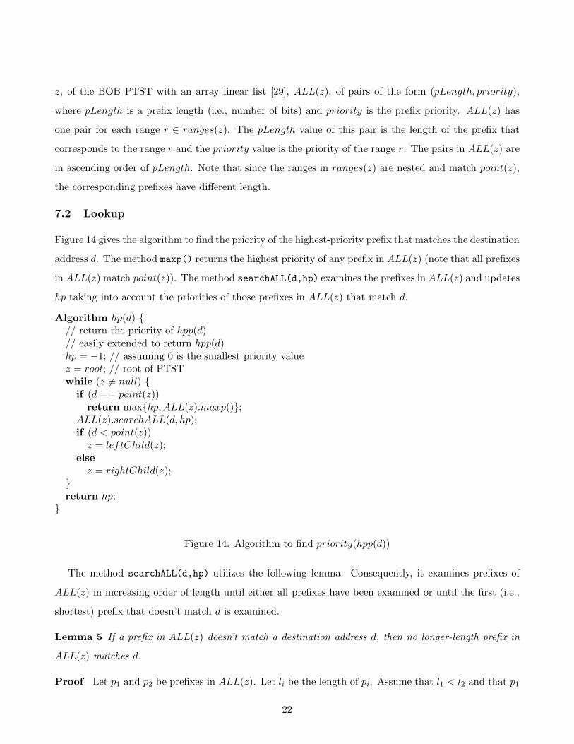
7.2 Lookup

Figure 14 gives the algorithm to find the priority of the highest-priority prefix that matches the destination

address d. The method maxp() returns the highest priority of any prefix in ALL(z) (note that all prefixes

in ALL(z) match point(z)). The method searchALL(d,hp) examines the prefixes in ALL(z) and updates

hp taking into account the priorities of those prefixes in ALL(z) that match d.

Algorithm hp(d) {// return the priority of hpp(d)// easily extended to return hpp(d)hp = −1; // assuming 0 is the smallest priority valuez = root; // root of PTSTwhile (z 6= null) {

if (d == point(z))return max{hp,ALL(z).maxp()};

ALL(z).searchALL(d, hp);if (d < point(z))

z = leftChild(z);else

z = rightChild(z);}return hp;

}

Figure 14: Algorithm to find priority(hpp(d))

The method searchALL(d,hp) utilizes the following lemma. Consequently, it examines prefixes of

ALL(z) in increasing order of length until either all prefixes have been examined or until the first (i.e.,

shortest) prefix that doesn’t match d is examined.

Lemma 5 If a prefix in ALL(z) doesn’t match a destination address d, then no longer-length prefix in

ALL(z) matches d.

Proof Let p1 and p2 be prefixes in ALL(z). Let li be the length of pi. Assume that l1 < l2 and that p1

22

doesn’t match d. Since both p1 and p2 match point(z), p2 is nested within p1. Therefore, all destination

addresses that are matched by p2 are also matched by p1. So, p2 doesn’t match d.

One way to determine whether a length l prefix of ALL(z) matches d is to use the following lemma.

The check of this lemma may be implemented using a mask to extract the most-significant bits of point(z)

and d.

Lemma 6 A length l prefix p of ALL(z) matches d iff the most-significant l bits of point(z) and d are

the same.

Proof Straightforward.

Complexity We assume that the masking operations can be done in O(1) time each. (In IPv4, for

example, each mask is 32 bits long and we may extract any subset of bits from a 32-bit integer by taking

the logical and of the appropriate mask and the integer.) The number of PTST nodes reached in the

while loop of Figure 14 is O(log n) and the time spent at each node z that is reached is linear in the

number of prefixes in ALL(z) that match d. Since the PTST has at most maxR prefixes that match

d, the complexity of our lookup algorithm is O(log n + maxR) = O(W ) (note that log2 n ≤ W and

maxR ≤ W ).

7.3 Insertion and Deletion

The PBOB algorithms to insert/delete a prefix are simple adaptations of the corresponding algorithms

for BOB. rMax is found by examining the prefixes in ALL(x) in increasing order of length. ALL′(y) is

obtained by prepending the prefixes in ALL(x) whose length is ≤ the length of rMax to ALL(y), and

ALL′(x) is obtained from ALL(x) by removing the prefixes whose length is ≤ the length of rMax. The

time require to find rMax is O(maxR). This is also the time required to compute ALL′(y) and ALL′(x).

The overall complexity of an insert/delete operation is O(log n + maxR) = O(W ).

As noted earlier, maxR ≤ 6 in practice. So, in practice, PBOB takes O(log n) time and makes O(log n)

cache misses per operation.

8 Longest-Matching Prefix-Tables (LMPTs)—LMPBOB

8.1 The Data Structure

Using priority = pLength, a PBOB may be used to represent an LMPT obtaining the same performance

as for an HPPT. However, we may achieve some reduction in the memory required by the data structure

23

if we replace the array linear list that is stored in each node of the PTST by a W -bit vector, bit. bit(z)[i]

denotes the ith bit of the bit vector stored in node z of the PTST, bit(z)[i] = 1 iff ALL(z) has a prefix

whose length is i. We note that Suri et al. [20] use W -bit vectors to keep track of prefix lengths in their

data structure also.

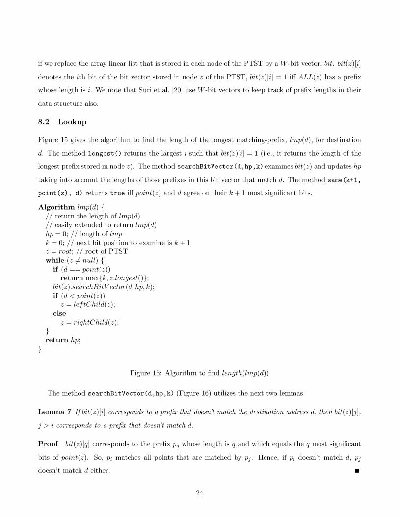
8.2 Lookup

Figure 15 gives the algorithm to find the length of the longest matching-prefix, lmp(d), for destination

d. The method longest() returns the largest i such that bit(z)[i] = 1 (i.e., it returns the length of the

longest prefix stored in node z). The method searchBitVector(d,hp,k) examines bit(z) and updates hp

taking into account the lengths of those prefixes in this bit vector that match d. The method same(k+1,

point(z), d) returns true iff point(z) and d agree on their k + 1 most significant bits.

Algorithm lmp(d) {// return the length of lmp(d)// easily extended to return lmp(d)hp = 0; // length of lmp

k = 0; // next bit position to examine is k + 1z = root; // root of PTSTwhile (z 6= null) {

if (d == point(z))return max{k, z.longest()};

bit(z).searchBitV ector(d, hp, k);if (d < point(z))

z = leftChild(z);else

z = rightChild(z);}return hp;

}

Figure 15: Algorithm to find length(lmp(d))

The method searchBitVector(d,hp,k) (Figure 16) utilizes the next two lemmas.

Lemma 7 If bit(z)[i] corresponds to a prefix that doesn’t match the destination address d, then bit(z)[j],

j > i corresponds to a prefix that doesn’t match d.

Proof bit(z)[q] corresponds to the prefix pq whose length is q and which equals the q most significant

bits of point(z). So, pi matches all points that are matched by pj . Hence, if pi doesn’t match d, pj

doesn’t match d either.

24

Algorithm searchBitV ector(d, hp, k) {// update hp and k

while (k < W and same(k + 1, point(z), d)) {if (bit(z)[k + 1] == 1)

hp = k + 1;k + +;

}}

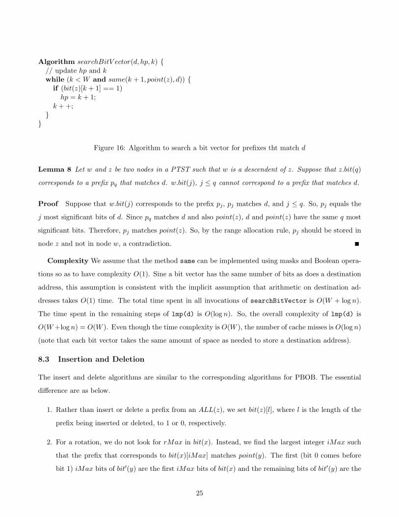
Figure 16: Algorithm to search a bit vector for prefixes tht match d

Lemma 8 Let w and z be two nodes in a PTST such that w is a descendent of z. Suppose that z.bit(q)

corresponds to a prefix pq that matches d. w.bit(j), j ≤ q cannot correspond to a prefix that matches d.

Proof Suppose that w.bit(j) corresponds to the prefix pj, pj matches d, and j ≤ q. So, pj equals the

j most significant bits of d. Since pq matches d and also point(z), d and point(z) have the same q most

significant bits. Therefore, pj matches point(z). So, by the range allocation rule, pj should be stored in

node z and not in node w, a contradiction.

Complexity We assume that the method same can be implemented using masks and Boolean opera-

tions so as to have complexity O(1). Sine a bit vector has the same number of bits as does a destination

address, this assumption is consistent with the implicit assumption that arithmetic on destination ad-

dresses takes O(1) time. The total time spent in all invocations of searchBitVector is O(W + log n).

The time spent in the remaining steps of lmp(d) is O(log n). So, the overall complexity of lmp(d) is

O(W +log n) = O(W ). Even though the time complexity is O(W ), the number of cache misses is O(log n)

(note that each bit vector takes the same amount of space as needed to store a destination address).

8.3 Insertion and Deletion

The insert and delete algorithms are similar to the corresponding algorithms for PBOB. The essential

difference are as below.

1. Rather than insert or delete a prefix from an ALL(z), we set bit(z)[l], where l is the length of the

prefix being inserted or deleted, to 1 or 0, respectively.

2. For a rotation, we do not look for rMax in bit(x). Instead, we find the largest integer iMax such

that the prefix that corresponds to bit(x)[iMax] matches point(y). The first (bit 0 comes before

bit 1) iMax bits of bit′(y) are the first iMax bits of bit(x) and the remaining bits of bit′(y) are the

25

same as the corresponding bits of bit(y). bit′(x) is obtained from bit(x) by setting its first iMax

bits to 0.

Complexity iMax may be determined in O(log W ) time using binary search; bit′(x) and bit′(y) may

be computed in O(1) time using masks and boolean operations. The remaining tasks performed during

an insert or delete take O(log n) time. So, the overall complexity of an insert or delete operation is

O(log n + log W ) = O(log(Wn)). The number of cache misses is O(log n).

9 Experimental Results

Test Data and Memory Requirement

We implemented the BOB, PBOB, and LMPBOB data structures and associated algorithms in C++

and measured their performance on a 1.4 GHz PC. In our implementation, each node is aligned to a

4-byte memory boundary and we use a byte as the basic unit for each field in a node. For example, we

use 1 byte for the color field of a red-black node even though 1 bit suffices. We use 4 bytes for child

pointer fields.

To assess the performance of these data structures, we used six IPv4 prefix databases obtained from

[30]5. We assigned each prefix a priority equal to its length. Hence, BOB, PBOB, and LMPBOB were all

used in a longest matching-prefix mode. For dynamic router-tables that use the longest matching-prefix

tie breaker, the PST structure of Lu and Sahni [24] provides O(log n) lookup, insert, and delete. So, we

included the PST in our experimental evaluation of BOB, PBOB, and LMPBOB.

The number of prefixes in each of our 6 databases as well as the memory requirement for each

database of prefixes are shown in Table 2. For the memory requirement, we performed two measurements.

Measure1 gives the memory used by a data structure that is the result of a series of insertions made into

an initially empty instance of the data structure. For Measure1, less than 1% of the PTST-nodes in the

constructed BOB, PBOB, and LMPBOB instances are empty. So, these data structures use close to the

minimum amount of memory they could use. Measure2 gives the memory used after 75% of the prefixes

in the data structure constructed for Measure1 are deleted. In the resulting BOB, PBOB, and LMPBOB

instances, almost half the PTST nodes are empty. The databases Paix1, Pb1, MaeWest and Aads were

obtained on Nov 22, 2001, while Pb2 and Paix2 were obtained Sep 13, 2000. Figure 17 histograms

the data of Table 2. The memory required by PBOB and LMPBOB is the same when rounded to the

5Our experiments are limited to prefix databases because range databases are not available for benchmarking. Although,we could randomly generate a database of ranges, this database is unlikely to have nesting properties similar to that of realdatabases [2].

26

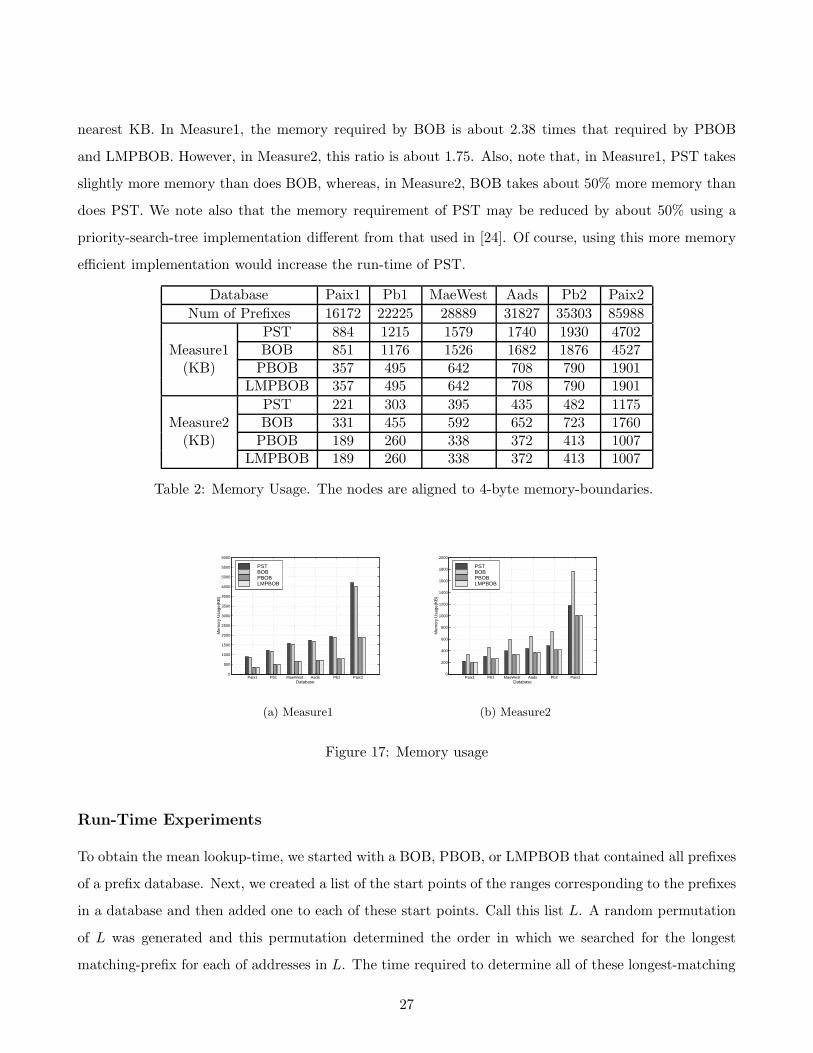
nearest KB. In Measure1, the memory required by BOB is about 2.38 times that required by PBOB

and LMPBOB. However, in Measure2, this ratio is about 1.75. Also, note that, in Measure1, PST takes

slightly more memory than does BOB, whereas, in Measure2, BOB takes about 50% more memory than

does PST. We note also that the memory requirement of PST may be reduced by about 50% using a

priority-search-tree implementation different from that used in [24]. Of course, using this more memory

efficient implementation would increase the run-time of PST.

Database Paix1 Pb1 MaeWest Aads Pb2 Paix2

Num of Prefixes 16172 22225 28889 31827 35303 85988

PST 884 1215 1579 1740 1930 4702Measure1 BOB 851 1176 1526 1682 1876 4527

(KB) PBOB 357 495 642 708 790 1901LMPBOB 357 495 642 708 790 1901

PST 221 303 395 435 482 1175Measure2 BOB 331 455 592 652 723 1760

(KB) PBOB 189 260 338 372 413 1007LMPBOB 189 260 338 372 413 1007

Table 2: Memory Usage. The nodes are aligned to 4-byte memory-boundaries.

Paix1 Pb1 MaeWest Aads Pb2 Paix2 0

500

1000

1500

2000

2500

3000

3500

4000

4500

5000

5500

6000

Database

Mem

ory

Usa

ge(K

B)

PSTBOBPBOBLMPBOB

(a) Measure1

Paix1 Pb1 MaeWest Aads Pb2 Paix2 0

200

400

600

800

1000

1200

1400

1600

1800

2000

Database

Mem

ory

Usa

ge(K

B)

PSTBOBPBOBLMPBOB

(b) Measure2

Figure 17: Memory usage

Run-Time Experiments

To obtain the mean lookup-time, we started with a BOB, PBOB, or LMPBOB that contained all prefixes

of a prefix database. Next, we created a list of the start points of the ranges corresponding to the prefixes

in a database and then added one to each of these start points. Call this list L. A random permutation

of L was generated and this permutation determined the order in which we searched for the longest

matching-prefix for each of addresses in L. The time required to determine all of these longest-matching

27

prefixes was measured and averaged over the number of addresses in L (actually, since the time to

perform all these lookups was too small to measure accurately, we repeated the lookup for all addresses

in L several times and then averaged). The experiment was repeated ten times, each time using different

random permutation of L, and the mean and standard deviation of these average times computed. These

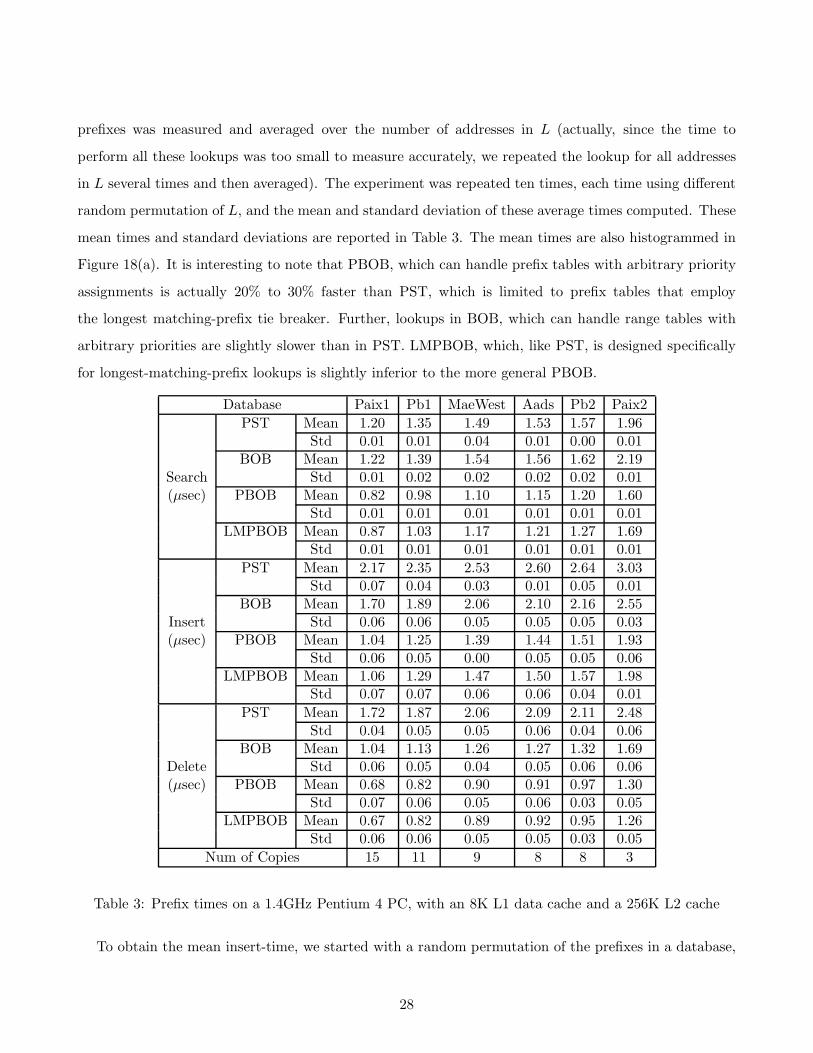
mean times and standard deviations are reported in Table 3. The mean times are also histogrammed in

Figure 18(a). It is interesting to note that PBOB, which can handle prefix tables with arbitrary priority

assignments is actually 20% to 30% faster than PST, which is limited to prefix tables that employ

the longest matching-prefix tie breaker. Further, lookups in BOB, which can handle range tables with

arbitrary priorities are slightly slower than in PST. LMPBOB, which, like PST, is designed specifically

for longest-matching-prefix lookups is slightly inferior to the more general PBOB.

Database Paix1 Pb1 MaeWest Aads Pb2 Paix2

PST Mean 1.20 1.35 1.49 1.53 1.57 1.96Std 0.01 0.01 0.04 0.01 0.00 0.01

BOB Mean 1.22 1.39 1.54 1.56 1.62 2.19Search Std 0.01 0.02 0.02 0.02 0.02 0.01(µsec) PBOB Mean 0.82 0.98 1.10 1.15 1.20 1.60

Std 0.01 0.01 0.01 0.01 0.01 0.01LMPBOB Mean 0.87 1.03 1.17 1.21 1.27 1.69

Std 0.01 0.01 0.01 0.01 0.01 0.01

PST Mean 2.17 2.35 2.53 2.60 2.64 3.03Std 0.07 0.04 0.03 0.01 0.05 0.01

BOB Mean 1.70 1.89 2.06 2.10 2.16 2.55Insert Std 0.06 0.06 0.05 0.05 0.05 0.03(µsec) PBOB Mean 1.04 1.25 1.39 1.44 1.51 1.93

Std 0.06 0.05 0.00 0.05 0.05 0.06LMPBOB Mean 1.06 1.29 1.47 1.50 1.57 1.98

Std 0.07 0.07 0.06 0.06 0.04 0.01

PST Mean 1.72 1.87 2.06 2.09 2.11 2.48Std 0.04 0.05 0.05 0.06 0.04 0.06

BOB Mean 1.04 1.13 1.26 1.27 1.32 1.69Delete Std 0.06 0.05 0.04 0.05 0.06 0.06(µsec) PBOB Mean 0.68 0.82 0.90 0.91 0.97 1.30

Std 0.07 0.06 0.05 0.06 0.03 0.05LMPBOB Mean 0.67 0.82 0.89 0.92 0.95 1.26

Std 0.06 0.06 0.05 0.05 0.03 0.05

Num of Copies 15 11 9 8 8 3

Table 3: Prefix times on a 1.4GHz Pentium 4 PC, with an 8K L1 data cache and a 256K L2 cache

To obtain the mean insert-time, we started with a random permutation of the prefixes in a database,

28

Paix1 Pb1 MaeWest Aads Pb2 Paix2 0

0.2

0.4

0.6

0.8

1

1.2

1.4

1.6

1.8

2

2.2

2.4

2.6

2.8

3

3.2

3.4

Database

Sea

rch

Tim

e (µ

sec)

PSTBOBPBOBLMPBOB

(a) Search

Paix1 Pb1 MaeWest Aads Pb2 Paix2 0

0.2

0.4

0.6

0.8

1

1.2

1.4

1.6

1.8

2

2.2

2.4

2.6

2.8

3

3.2

3.4

Database

Inse

rt T

ime

(µse

c)

PSTBOBPBOBLMPBOB

(b) Insert

Paix1 Pb1 MaeWest Aads Pb2 Paix2 0

0.2

0.4

0.6

0.8

1

1.2

1.4

1.6

1.8

2

2.2

2.4

2.6

2.8

3

3.2

3.4

Database

Rem

ove

Tim

e (µ

sec)

PSTBOBPBOBLMPBOB

(c) Delete

Figure 18: Execution Time

inserted the first 67% of the prefixes into an initially empty data structure, measured the time to insert

the remaining 33%, and computed the mean insert time by dividing by the number of prefixes in 33% of

the database. (Once again, since the time to insert the remaining 33% of the prefixes was too small to

measure accurately, we started with several copies of the data structure and inserted the 33% prefixes

into each copy; measured the time to insert in all copies; and divided by the number of copies and

number of prefixes inserted). This experiment was repeated ten times, each time starting with a different

permutation of the database prefixes, and the mean of the mean as well as the standard deviation in the

mean computed. These latter two quantities as well as the number of copies of each data structure we

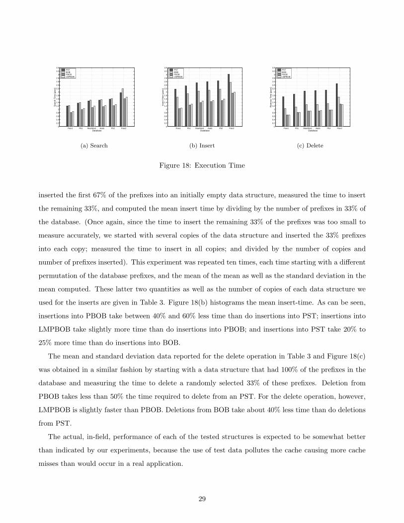
used for the inserts are given in Table 3. Figure 18(b) histograms the mean insert-time. As can be seen,

insertions into PBOB take between 40% and 60% less time than do insertions into PST; insertions into

LMPBOB take slightly more time than do insertions into PBOB; and insertions into PST take 20% to

25% more time than do insertions into BOB.

The mean and standard deviation data reported for the delete operation in Table 3 and Figure 18(c)

was obtained in a similar fashion by starting with a data structure that had 100% of the prefixes in the

database and measuring the time to delete a randomly selected 33% of these prefixes. Deletion from

PBOB takes less than 50% the time required to delete from an PST. For the delete operation, however,

LMPBOB is slightly faster than PBOB. Deletions from BOB take about 40% less time than do deletions

from PST.

The actual, in-field, performance of each of the tested structures is expected to be somewhat better

than indicated by our experiments, because the use of test data pollutes the cache causing more cache

misses than would occur in a real application.

29

10 Conclusion

We have proposed an enhancement of the interval tree structure of [28]. Our enhancement permits nodes

that are empty (i.e., contain no range) but requires there be at most 2n nodes in the interval tree. The

enhanced structure supports efficient insertion and deletion of ranges. Several data structures, based on

this enhanced interval tree, have been proposed for the representation of dynamic IP router-tables.

Our experiments show that PBOB is to be preferred over PST and LMPBOB for the representation of

dynamic longest-matching prefix-router-tables. This is somewhat surprising because PBOB may be used

for highest-priority prefix-router-tables, not just longest-matching prefix-router-tables. A possible reason

why PBOB is faster than LMPBOB is that in LMPBOB one has to check O(W ) prefix lengths, whereas

in PBOB O(maxR) lengths are checked (note that in our test databases, W = 32 and maxR ≤ 6). BOB

is slower than and requires more memory than PBOB when tested with longest-matching prefix-router

tables. The same relative performance between BOB and PBOB is expected when filters are prefixes

with arbitrary priority. Of the data structures considered in this paper, BOB or CBOB may be used

when the filters are ranges that have an associated priority.

References

[1] C. Macian and R. Finthammer. An evaluation of the key design criteria to achieve high update

rates in packet classifiers. IEEE Network, pages 24–29, Nov./Dec. 2001.

[2] F. Baboescu, S. Singh, and G. Varghese. Packet classification for core routers: is there an alternative

to cams? In IEEE INFOCOM, 2003.

[3] C. Labovitz, G. Malan, and F. Jahanian. Internet routing instability. IEEE/ACM Transactions on

Networking, 1997.

[4] M. Ruiz-Sanchez, E. Biersack, and W. Dabbous. Survey and taxonomy of ip address lookup algo-

rithms. IEEE Network, 15(2):8–23, March/April 2001.

[5] S. Sahni, K. Kim, and H. Lu. Data structures for one-dimensional packet classification using most-

specific-rule matching. In International Symposium on Parallel Architectures, Algorithms, and Net-

works (ISPAN), May 2002.

[6] A. McAuley and P. Francis. Fast routing table lookups using cams. In IEEE INFOCOM, pages

1382–1391, 1993.

30

[7] D. Shah and P. Gupta. Fast updating algorithms for tcams. IEEE MICRO, 21(1):36–47, 2001.

[8] C. Matsumoto. Cam vendors consider algorithmic alternatives. EETimes, May 2002.

[9] K. Sklower. A tree-based routing table for berkeley unix. Technical report, University of California

- Berkeley, 1993.

[10] M. Degermark, A. Brodnik, S. Carlsson, and S. Pink. Small forwarding tables for fast routing

lookups. In ACM SIGCOMM, pages 3–14, 1997.

[11] W. Doeringer, G. Karjoth, and M. Nassehi. Routing on longest-matching prefixes. IEEE/ACM

Transactions on Networking, 4(1):86–97, 1996.

[12] S. Nilsson and G. Karlsson. Fast address look-up for internet routers. IEEE Broadband Communi-

cations, 1998.

[13] V. Srinivasan and G. Varghese. Faster ip lookups using controlled prefix expansion. ACM Transac-

tions on Computer Systems, pages 1–40, Feb 1999.

[14] S. Sahni and K. Kim. Efficient construction of fixed-stride multibit tries for ip lookup. In Proceedings

8th IEEE Workshop on Future Trends of Distributed Computing Systems, 2001.

[15] S. Sahni and K. Kim. Efficient construction of variable-stride multibit tries for ip lookup. In

Proceedings IEEE Symposium on Applications and the Internet (SAINT), 2002.

[16] P. Gupta, S. Lin, and N. McKeown. Routing lookups in hardware at memory access speeds. In

IEEE INFOCOM, 1998.

[17] M. Waldvogel, G. Varghese, J. Turner, and B. Plattner. Scalable high speed ip routing lookups. In

ACM SIGCOMM, pages 25–36, 1997.

[18] B. Lampson, V. Srinivasan, and G. Varghese. Ip lookup using multi-way and multicolumn search.

In IEEE INFOCOM, 1998.

[19] A. Basu and G. Narlika. Fast incremental updates for pipelined forwarding engines. In IEEE

INFOCOM, 2003.

[20] S. Suri, G. Varghese, and P. Warkhede. Multiway range trees: Scalable ip lookup with fast updates.

In GLOBECOM, 2001.

31

[21] S. Sahni and K. Kim. o(log n) dynamic packet routing. In IEEE Symposium on Computers and

Communications, 2002.

[22] S. Sahni and K. Kim. Efficient dynamic lookup for bursty access patterns. In

http://www.cise.ufl.edu/∼sahni, 2003.

[23] F. Ergun, S. Mittra, S. Sahinalp, J. Sharp, and R. Sinha. A dynamic lookup scheme for bursty

access patterns. In IEEE INFOCOM, 2001.

[24] H. Lu and S. Sahni. o(log n) dynamic router-tables for prefixes and ranges. In IEEE Symposium on

Computers and Communications, 2003.

[25] E. Horowitz, S. Sahni, and D. Mehta. Fundamentals of Data Structures in C++. W.H. Freeman,

New York, 1995.

[26] P. Gupta and N. McKeown. Dynamic algorithms with worst-case performance for packet classifica-

tion. In IFIP Networking, 2000.

[27] T. Cormen, C. Lieserson, R. Rivest, and C. Stein. Introduction to Algorithms. MIT Press, second

edition edition, 2001.

[28] M. D. Berg, M. V. Kreveld, M. Overmars, and O. Schwarzkopf. Computational Geometry: Algo-

rithms and Applications. Springer Verlag, 1997.

[29] S. Sahni. Data structures, algorithms, and applications in Java. McGraw Hill, New York, 2000.

[30] Merit. Ipma statistics. In http://nic.merit.edu/ipma, 2000, 2001.

32