131

CHAPTER – 6 EVOLVING JIT IMPLIMENTATION STRATEGIES

This chapter has been presenting the inferences drawn from literature, empirical

study carried out in Indian manufacturing industry and case study conducted in the

manufacturing organization. Inferences drawn from the survey and case study have been

synthesized to evolve critical success factors for strategic JIT implementation for Indian

Manufacturing industries. The SWOT analysis of JIT implementation in Indian

industries has also been presented in this chapter.

6.1 Strategies and success factors for overcoming challenges in JIT

implementation in Indian manufacturing industry

6.1.1 Just in time manufacturing

JIT is a method of production that developed out to evolve a defect free process

(see Chen and Podolsky, 1996). Horngren and Forster (1987) identified four major

objectives of JIT i.e., elimination of all process/activities that do not add value to

product or service, high level of quality, continuous improvement in the efficiency of

process/activity and stress on simplification and increased visibility to identify

process/activities that do not add value. Whereas according to Alawode and Ojo (2008)

the JIT philosophy is founded upon three fundamental principles, elimination of waste,

continuous quality improvements and encouragement of workers participation in

operations planning and execution. JIT is a Japanese-developed manufacturing

philosophy emphasizing excellence through the continuous elimination of waste and

improvement in productivity (Fullerton and McWatters, 2002). The primary motivation

for adopting JIT practices has been to reduce and ultimately eliminate waste, enhance

the quality of the product and improve delivery efficiency (Ahmad et al., 2003). Peters

and Austin (1995) suggested that reduction of buffer inventory between process means

closer integration and synchronisation is required. The waste is anything belongs to the

production process that does not add worth to the final product. Thus, waste includes

quality defects, inventories of all kinds, time spent to move material and time spent

setting up machines (Demmy and Gordon, 1988). Peters and Austin (1995) suggested

that reduction of waste or buffer inventory between process means closer integration

132

and synchronisation is required. Toyota Production system has given three broad types

of waste and these are Muda, Mura and Muri. The notion of JIT production was

described by Taiichi Ohno, the godfather of Toyota production system, as All we are

doing at the time line from the moment the customer gives us an order to the point when

we collect the cash and we are reducing that time line by removing the non-value-added

wastes (Liker, 2004).Many researchers have investigated the performance measures and

obstacles faced by an organisation while implementing JIT. Claycomb et al. (1999) in

his research work found that most commonly cited theoretical advantage of JIT is

inventory reduction. But reduction of waste is listed as the most important benefit of

JIT. Waste may be of raw material, waste during production or process and waste of

finished goods. Unlike traditional forms of manufacturing, where fabrication or

assembly takes place on the basis of materials availability (Mullarkey et al., 1995), JIT

is a ‘pull’ system of production where manufacturing only takes place when there are

needs from downstream operations and specific demands from customers. Thus, a major

aim of JIT is to produce and deliver final products just in time to be sold, subassemblies

just in time to be assembled into final products, fabricated parts just in time to go into

subassemblies and purchased materials just in time to be converted into fabricated parts

(Schonberger, 1982a). According to Davy et al. (1992) JIT production includes

following factors: focused factory; reduced setup times; group technology; total

preventive maintenance; uniform workloads; kanban; total quality control; quality

circles. The basic benefit of this manufacturing system is its ability to enhance the

organisation’s ability to compete with others, since with JIT, optimal process can be

developed for the firms. JIT also increases efficiency within the production thus reduces

costs of production also and it reduces waste of men machine, materials, time and effort.

A number of other benefits of JIT such as straitening firm’s culture and values,

improved coordination and relationship of supplier’s, reduction in inventory levels,

more product variety/flexibility, reduction in setup time, better maintenance of

equipment and machinery, delivery compliance and quality improvements.

Despite these benefits, the implementation of JIT production system in the third

world countries is limited because of several operational and systemic deficiencies.

Clark and Mia (1993) listed following difficulties in implementation of JIT like supplier

or customer inflexibility, staff resistance to change in existing systems, difficulties or

133

unexpected costs in the reorganisation of production facilities, prohibitive capital

requirements.

6.1.2 Obstacles to JIT implementation

The literature has revealed that that implementation of JIT is not an easy task by

any means. The failure of JIT implementation is due to lack of a support system to

facilitate learning and transform learning into effective diffusion of the practices of JIT

(Ahuja and Khamba, 2008). It has been found that many of the organisations that tries to

implement initiatives faces difficulties and are not able to achieve the required benefits.

The failure of an organisation to implement a JIT program successfully has been

imputed to the various obstacles that include lack of management support and

understanding, lack of sufficient/proper training, failure to allow sufficient time for the

evolution (Bakerjan, 1994). Some of the major problems in JIT implementation include

partial implementation of JIT, overly optimistic expectations, lack of cooperation from

vendors in a form of inconsistent timing and quantities of deliveries, lack of resources to

invest in direct linkages with vendors, the unwillingness of workers to perform multi-

tasks, management’s resistance to sharing operational power with employees, lack of

management confidence in hourly workers’ commitment to the organisation; and the

lack of accurate forecasting system (Yasin et al., 2004). The intensity of problems

associated with materials and information flow has been reduced in effectively

implemented JIT manufacturing system. On the other hand, new problems for employee

used to arise when any new system or technology is introduced. This phenomenon is in

keeping with ‘socio technical’ theories (Susman and Chase, 1986) and anecdotal

descriptions of JIT implementation problems have suggested that it may occur

frequently (Bailey and Rose, 1988; Heiko, 1989; Hendrick, 1988; Majchrzak, 1988). For

example, employees in a JIT system are highly dependent both on other group members

and on reliable systems for information exchange (Ahuja and Khamba, 2008).

Additionally, Employee has to perform wider range of job functions when they move

from a functional layout to a cellular JIT layout. Thus, we anticipated that some

performance obstacles, such as material delivery, would decrease with JIT, while others

– such as interdependence caused by waiting for co-workers to complete preceding

procedures – would increase (Ahuja and Khamba, 2008).

134

6.1.3 Success factors for successful JIT implementation

In today’s manufacturing environment, the manufacturing organisation is

considered an open, productive, dynamic information system (Yasin and Wafa, 1996).

So in a highly competitive global business scenario, the aim of the manufacturing

organisation is long term survival. To survive, the manufacturing organisations must be

willing to make tactful adjustments consistent with the demands of its environment

(Yasin and Wafa, 1996). JIT is the one of techniques used by manufacturing

organisations to remain competent with their rivals.

It is clear from the research that a JIT philosophy has the potential for increasing

organisational efficiency and effectiveness. Specifically, the following potential benefits

of JIT are cited in the literature: lower materials and finished goods inventory levels

(Clark and Mia, 1993), very low work-in-process inventories (Clark and Mia, 1993),

reductions in materials handling costs (Clark and Mia, 1993), eliminate waste in

production and material (Natarajan, 1991; Tesfay, 1990), improves communication

internally (in the organisation) and externally (between the organisation and its

customers and vendors (Inman and Mehra, 1991).

Successful application of the JIT manufacturing is assumed to lead to

improvements in both financial and non-financial performance such as lower production

costs, higher and faster throughput and improved product quality and on-time delivery

of products, which should ultimately result in improved profitability (Fullerton et al.,

2003). It has been argued by many that adoption of JIT philosophy might lead to

improved operations in an organisation but does not necessarily always result in higher

profitability (Johnson and Kaplan, 1989) particularly over a short term period. Cooper

(1987) explained that by implementing JIT companies should not expect financial

benefits over a short term period but they could instead learn from the Japanese

counterparts who stress more on stability, long-term reliability and growth. Johnson and

Bröms (2000) reveal in his work that it is Toyota’s manufacturing practices that

promote growth and stability over the long run and not the achievement of short-run

financial targets that contribute to its stable performance. Thus, the focus on financial

performance alone is not sufficient for firms to survive and excel in today’s market (Isa,

2011). Some of the benefits reported by Yasin et al. (2004) are reduction in work-

135

in-process inventory, improved material flow and throughput, reduced lead-times,

improvement in the quality level of incoming material, less paperwork, significant

reduction in rejects of outgoing final products/services and reduction in the number of

grievances filed by workers.

In manufacturing, JIT has been credited with many holistic benefits. These

benefits include reduced inventory levels; reduced investment in inventory; improved

quality of incoming materials; and consistent high-quality products. Some additional

benefits of JIT that have been achieved in manufacturing firms are: improved

operational efficiency, uniform workstation loads; standardised components;

standardised work methods; cooperative relationships with suppliers; closer

collaboration with customers and improved customer satisfaction (Yasin et al., 2004).

Abdallah and Matsui (2007) suggested following performance measures of JIT and

these are on time delivery performance, flexibility to change volume, inventory turnover

and cycle time. Whereas Manoj (2011) observed that by implementing JIT various types

of inventories like raw material inventory, work in process inventory and finishes goods

inventory got reduced drastically in Indian manufacturing industries.

However, there have not been many references to strategic initiatives for

overcoming the limitations to successful JIT implementation in the Indian context. Thus

this study assumes significance since it lay stress on evolution of key success factors for

overcoming the obstacles to JIT implementation in the Indian manufacturing industry.

6.1.4 Challenges for JIT implementation in Indian manufacturing industry

… JIT is something that is already implemented in the industries of India

without much knowhow what JIT actually means (Telsan et al., 2006)

As the organisations across the world have faced stiff cut-throat competition in

the last three decades, the Indian industry too could not escape the brunt of globalisation

(Ahuja and Khamba, 2008). Due to entry of multinational companies since early 1990’s,

Indian manufacturing industry has also witness’s stiff competition in recent times.

Owing to opening up of the Indian economy from merely a regulated economy, the

manufacturing industry has been faced with uphill task of competing with the best in the

world (Ahuja and Khamba, 2008). The competition worldwide has been witnessed in

136

terms of lowering of costs, improved quality and products with high performance

(Chandra and Sastry, 1998).

Moreover reducing lead times and setup time, innovation times and controlling

inventories have lead to increasing demands on the organisation’s preparedness,

adaptability and versatility.

Indian manufacturing sector is one of the largest industrial powers of the word,

which has never been allowed to realise its potential due to the interference of

bureaucratic governments and protectionists (Kumar, 2010). Due to this Indian goods

are unable to compete with the product of other countries. Traditionally, Indian

manufacturing organisations have suffered from inherent problems like poor

responsiveness to changing market scenarios, low productivity, poor quality, poor cost

effectiveness of production systems, stubborn organisational character and structures,

uncertain policy regimes, low skill and knowledge base of employees, low production

automation, non-motivating work environments, high customer complaints, high utility

rates, high wastages associated with production systems, high labour rigidity, high

internal taxes and infrastructural glitches (Ahuja and Khamba, 2008). Challenge of cost

effective manufacturing strategies has to be adopted for staying competitive by Indian

industry (Chandra and Kodali, 1998). While implementing effective JIT manufacturing,

the Indian organisations have often been bothered with some problems and challenges

like difficulties to understand business economics, reluctance to change, worker’s

apprehensions of more work, management’s commitment and inability to realise the

same level of benefits as reaped by developed countries by imitating the JIT

implementation procedures and practices adopted abroad. Thus Indian manufacturing

organisations need to shed the sluggish character and move forward aggressively to

develop adapt proactive processes and practices for overcoming the inherent

deficiencies in manufacturing systems for harnessing distinct competencies in

comparison to their global competitors (Ahuja and Khamba, 2008). The present study

critically examines the factors effecting the implementation of JIT practices in Indian

manufacturing industry. Currently many models are undergoing failures and in this

situation this study is relevant. Implementation of JIT in Indian industry lead to an

enormous saving and creation of new productivity ethics which go in a long way to

strengthening of Indian economy (Singh and Garg, 2011). In addition to that Indian

137

industries become more competitive worldwide. But researchers have listed some issues

that can make or break the implementation of JIT manufacturing. Successful

implementation of JIT requires top management involvement and proper employee

training. Wakchaure et al. (2006) listed the major reasons pointed out for the slow

implementation by respondents are: Lack of information on JIT implementation, Lack

of justification for practicing JIT, Lack of assistance available from consulting firms and

government bodies, Lack of formal cross training program for workers, Problem in

maintenance time reduction, Initial high investment in layout improvement to suit JIT

requirements, JIT purchasing due to lack of infrastructure.

Venkatesh et al. (2007) listed the following difficulties in implementing JIT in

Indian: Lack of cooperation of suppliers in correctly supplied material, the lack of

resources to invest in direct linkages with vendors, Lack of formal cross training

programs for workers, Lack of formal training/education, Lack of cooperation from

vendors in the form of inconsistent lead times and capacity constraints imposed by

suppliers, Lack of an accurate forecasting system, Lack of strategic planning, Problem

in maintenance time reduction through machine, modification or replacement of existing

equipment, Quality problems with supplied material, Lack of cooperation of suppliers in

timing of supplied materials, Reduction in the levels of work load variability, Problems

with machines (Machine failures and reliability, Lack of information and

communication with suppliers, Inability to meet schedule, Lack of communication

between workers and management, Problem in line balancing, Lack of performance

measure, Problem in lead times reduction, Problems in layout modification, Lack of

team work spirit, Departmental conflicts, Poor quality. Whereas Malik et al. (2011)

listed following factors for the slow implementation of JIT: High cost of

implementation, Informal/casual quality auditing, On QC, lack of communication, Lack

of customer awareness on QC, Lack of employee participation, Lack of production

technology, Lack of support from workers, Lack of support from supervisors, Lack of

support from suppliers, Lack of support from designers, Lack of support from HRD,

Lack of support from R&D. Figure 6.1 elaborates the reasons for slow implementation

of JIT in Indian manufacturing industry.

138

Figure 6.1 Slow implementation of JIT in Indian manufacturing industries

6.1.5 Barriers to JIT implementation in Indian manufacturing industry

Some of the major organisational obstacles affecting the successful JIT

implementation in Indian manufacturing organisations include:

Organisation’s inability to bring about cultural transformation.

Lack of information on JIT implementation.

Ineffectiveness of top management to holistically implement change

management initiatives.

Lack of formal cross training program for workers.

139

Lack of commitment from top management and communication regarding JIT.

High initial investment in layout improvement to suit JIT requirements.

Lack of Infrastructure for JIT purchasing.

Lack of cooperation of suppliers to supply materials in time and frequently.

Lack of strategic planning.

Lack of Poka-yoke installation.

Inability to Kanban system installation.

Maintenance, machine failures and reliability.

The detailed observations regarding JIT implementation obstacles in Indian context are

listed below:

Obstacles regarding culture of an organisation: Culture of an organisation implies the

system of shared meaning, cooperating and the way one works and gets work done

under all circumstances. In every organisation there are some beliefs, norms, rituals,

actions, communication, ceremonies, behaviours, myths, sagas, activities, decision

making method, management style and practices that have been come into existence

over a period of time. Culture of an organisation plays a vital role in implementing JIT.

Figure 6.2 explain the barriers in implementing JIT due to culture on an organisation.

Figure 6.2 Obstacles related to culture of an organization

140

Obstacles related to employees involvement and commitment: The main aim of JIT is

to reduce waste and reduction or eliminate inventories. The reduction of inventory

between processes means closer integration and synchronisation is required between

workers. Due to this operators/worker’s latitude and freedom are reduced, creativity and

motivation may in turn also be reduced. Some of the issues that lead to barrier in JIT

implementation in an organisation are listed in Figure 6.3.

Figure 6.3 Obstacles related to employee’s involvement and commitment

Obstacles related to quality: The main aim of the quality control department is to make

sure that the level of defective parts leaving the shop floor should falls within specified

levels, the main objective is that defect should be detect at source as soon as it arise.

TQM is a production method with an aim of continuously improvement and

maintenance of quality of products and processes. This can be achieved by the

involvement of management, workers, suppliers and customers in order to meet

customer expectations. The difficulties related to quality in Indian context are listed in

Figure 6.4.

141

Figure 6.4 Obstacles related to quality

Plant and equipment/facility layout related obstacles: For ensuring the smooth and

continuous work flow from the raw material to finished products, it is necessary that

industry should adopt a product approach in spite of functional or process layout. To

prevent the accumulation of work in process various techniques of grouping the

faculties/equipment are used. To obstacles related to this are shown in Figure 6.5.

Figure 6.5 Obstacles related to plant and equipment/facility layout

Inventory management obstacles: The main aim of JIT is to eliminate or to reduce all

kind of inventories whether it is raw material, work in process or finished goods

inventories. High inventory holdings are commonly identified as poor management.

Figure 6.6 explains the obstacles related to inventory observed by Indian industries.

142

Figure 6.6 Inventory management obstacles

Obstacles related to process/production system: For the success of JIT

process/production strategies also plays an important role. Some of the obstacles related

to process are listed in Figure 6.7.

Figure 6.7 Obstacles related to process/production system

143

6.1.6 Success factors and enablers for successful JIT implementation

The new emerging technologies have far reaching impact for the competitive

advantages of countries in the global competition of international markets. Developing

countries like India cannot remain just silent spectator when this new industrial burst in

technology sweeps the industrialised world. In the present context, Indian

manufacturing organisations have risen to the occasion and progressed to envisage

efficient policies that helps an organisation to enhance production system reliability,

cost effectiveness of production operations, low cost of product with high quality so as

to enabling the organisations to realise competencies to meet the challenges posed by

global competition.

The success factors achieved by implementing JIT system are enhanced profi ts

and to get huge return on investment by reduction of input costs, reduction of inventory

and improvement in quality. But to achieve all these goals it has been observed strong

resistance from within. Indian manufacturing organisations have suffered due to lacking

organizational cultures, management commitment, low skill and knowledge of

operators, multi skill labour, inadequate resources and poor work environments. Indian

manufacturing organisations need to take many initiatives to overcome the barriers

mentioned earlier to ensure the realization of true potential of JIT. Thus it becomes

compulsory for the Indian organisations to develop proactive strategies for indigenous

JIT implementation program for the Indian industry. The key enablers and success

factors for implementation of JIT in Indian manufacturing industry can be classified into

ten categories:

Top management’s commitment and culture of an organization.

Employee’s involvement and commitment.

Supplier’s coordination and relationship.

Inventory levels.

Product variety and flexibility.

Set-up-time.

Production.

Maintenance of equipment.

144

Delivery compliance.

Quality.

The enables and success factors for implementation of JIT have been shown in

Figure 6.8. It is believed strongly that the adaptation of the above enablers and success

factors can reduce/ eliminate the ill effects of obstacles to JIT implementation and can

strategically lead the organisation to attain competencies for remaining competitive.

Support, commitment and involvement of top management are required for the

successful implementation of JIT. Commitment of top management should be required

to implement JIT program and they should evolve mechanisms for multi-level

communication to all employees and clarify the importance, objectives and benefits of

the whole program and whole heartedly advocate the benefits of JIT to the organisation.

The first step is to establish a strategic direction for JIT. A master plan should be

prepared for implementation of JIT.

This must be followed by designing JIT secretariat in accordance with

organisation’s policies involving employees from various organisation hierarchical

levels. The management contributions towards successful JIT implementations can

include revising business plans to include JIT goals, take steps to change culture of an

organisation, building strong success stories so that employees should be motivated for

JIT implementations, JIT goals should be communicating to the entire organisation,

providing adequate financial resources, promoting multi skill working in organisation,

providing training to workers, evolving reward and incentive system to motivate

workers, improvements and changes in workplace should be supported, barriers at the

middle level management should be removed, leadership and managerial skills should

be used instead of considering themselves as boss.

An organisation implementing JIT should consider workers as assets. They

should be given more authority and power to make decisions. The workers have to

perform a more varied role within the organisation because they are trained to perform

multi skill duties like flexibility in reducing bottlenecks as well as substituting for

absent co-workers. The worker has to perform the following additional duties in a JIT

environment:

Performing several different jobs that require multi-skilling.

145

Maintaining production and inventory control.

Inspecting own work.

Performing rework on non-conforming (defective) parts.

Setting up production equipment.

Executing preventive and light maintenance of the production equipment.

Receiving or giving training both on and off the job.

Figure 6.8 Success factors and enablers for JIT implementation in an organisation

JIT purchasing requires reliable and frequent deliveries in exact quantities In JIT

environment partnership has to be developed between supplier and customer so as to

involve the suppliers and customers into the efficient process of JIT (Gupta, 1990). For

the selection of supplier most relevant factors is not price but minimum defective goods

and quality should be the criteria. So while selecting supplier the criteria should be such

146

that there should be minimum waste, less inspection, low costs of freight (with

geographic proximity), less paper work and small lot size and frequent delivery.

Although small lot size and frequent delivery is an important factor in JIT environment

but quality assurance should be the most important perquisite to select the supplier.

Following strategies should be taken into consideration while purchasing in JIT

environment:

Suppliers strategies

o Few suppliers.

o Nearby suppliers.

o Training of suppliers.

o Repeat business with same suppliers.

o Clusters of remote suppliers.

o Encouraging suppliers to implement JIT.

o Minimum paper work.

Quantity strategies

o Small lot size with frequent deliveries.

o Suppliers should be encouraged to deliver exact quantity.

o Suppliers to be encouraged to produce in small lots.

Quality strategies

o Minimum product specifications to be imposed on supplier.

o Suppliers are to be helped to meet quality requirements.

o Suppliers should be encouraged to use quality check techniques like

process control charts or statistical.

Shipment strategies

o Shipping should be done in such a way so that there should be no delays

during shipping.

147

In Indian industries have conventionally believed that inventory is needed as

they help in smooth and efficient running of enterprises. Implementation of JIT in an

industry leads to low levels of inventory. It is observed from the survey that various

types of inventories like raw material inventory, work in process inventory and finish

goods inventory got reduced drastically by implementing JIT in Indian manufacturing

industries.

The successful implementation of JIT also leads to enhancement in product

variety, flexibility and production of an organisation. It has also been seen from the

responses that setup time and down time of equipment and machinery got reduced.

Quality of products also got enhanced as the scrap and rework of part got reduced

drastically.

Finally the concerted efforts should be made for affecting JIT performance

improvements through deploying feedback from customer and various departments,

relation with suppliers, focusing upon learning from existing equipments to new

systems, incorporating design related improvements, using various techniques like

kanban, kaizan, Heijunka etc., improving safety at workplace, improving workplace

organisation through focused 5S initiatives and integrating JIT with other performance

improvement initiatives.

Interpretations and Conclusions

It has been seen from the research that conventional Indian manufacturing

industries have somewhat agonize in the past, while attempting to implement strategic

JIT initiatives and practices, since it needs to bring about important cultural conversions

in the organisation for changing the mind sets of the employees. The study seriously

examines various obstacles that affect the implementation of JIT in Indian

manufacturing organisations successfully. The obstacles/difficulties faced by the

organisations have been categorised into organisational, cultural, behavioural,

operational, technological, financial and departmental obstacles. Enablers and success

factors for successful implementation of JIT in Indian manufacturing industry have been

evolved by critically analysing the issues/obstacles faced by industry. Nevertheless, it

has also been found in the study that successful implementation of JIT initiatives can be

realistically achieved in an Indian manufacturing enterprise by bringing out successful

cultural changes, commitment of management. In order to ensure the implementation of

148

JIT initiatives and practices in the Indian manufacturing environments successfully, the

organisations must be willing to cultivate an environment that is ready to support

change in the workplace and create support for JIT concepts. Contributions of top

management’s contributions have been found to be highly important for implementation

of JIT successfully. Managers must know how to use JIT initiatives in the different

situations so as to develop involvement of employee in every step of the manufacturing

process and facilities smooth flow of product, improve product quality, reduce operating

costs, reduction in scrap and rework and low down time of equipment. Moreover, it can

be concluded from the research that the successful JIT implementation in an

organisations need to implement initiatives successfully so as to enhance organisation’s

productivity, improve maintenance performance, reduce costs, enhance quality of

product, improve plant profitability, minimise unnecessary downtime, ensure

participation of workers, ensure better utilisation of resources, thereby enhancing the

competitiveness of the organisation.

6.2 Selection of Performance Measure in JIT through Fuzzy Logic Based

Simulation

The study has been conducted by using Fuzzy Logic Toolbox of MATLAB and

fuzzy inference system for determination of significant performance measures by using

fuzzy interface system. The fuzzy toolbox helps developing models of complex system

behaviors using simple logic rules, and then those rules are implementing in a fuzzy

inference system. The study has focused on finding out significant performance

measures Fuzzy Based Simulation (FBS) model. Therefore, the most important factors

that affect the performance measures of any organization like percentage of JIT

implementation and percentage gain in performance measure by implementing JIT are

taken into account as input factors and in output following performance measures are

taken into account. These factors had been taken after considering the view points of JIT

coordinators from different manufacturing industries.

A suitable method to identify significant performance measures is expressed by

the following equation:

Significant Performance measure/s = f [percentage JIT implemented, percentage gain in

Performance measure] ……………………Eq. 6.1

Therefore the above equation is further optimized with use of fuzzy logic.

149

6.2.1 Brief Introduction of Fuzzy logic (FL)

The basic of Fuzzy logic begins with the concept of a fuzzy set. Whereas fuzzy

set is defined as a set that have no crisp, clearly defined boundary. It contains elements

which have only partial degree of membership. On the other hand, a membership

function (MF) is a curve that explains how each point in the input space is mapped to a

membership value (or degree of membership) between 0 and 1. The only condition a

membership function must satisfy is that it must lie between 0 and 1.

The membership function itself can be arbitrary curves shape of which can be defined as

a function that more appropriate from the simplicity, convenience, speed, and efficiency

point of view. It is a mathematical representation of the relationship between the input

and output of a system or a process. It also helps to facilitate the optimization of process

output by defining the relation- ship between input and the output variables. In the

context Optimization means minimizing the requirement in variability and shifting the

mean to some desired target value specified by the end user or customer. The function

presented in equation 1 is formulized and refined with the use of fuzzy logic. However,

in present study the refined function is acquainted as sets (sequences) of fuzzy logic

rules evaluated using the MATLAB’s fuzzy logic toolbox. Figure 6.9 shows the

graphical user interface (GUI) tool of Fuzzy Logic Toolbox to build a Fuzzy Inference

System (FIS). Fuzzy Logic may be described as a methodology for computing with

words rather than numbers. Although words are basically less precise than numbers as

their use is closer to human factor. Furthermore, computing with words exploits the

tolerance for imprecision and thereby lowers the cost of solution.

Another major concept in FL that plays a central role in most of its applications

is known as fuzzy if-then rule or, simply fuzzy rule. Although in Artificial Intelligence

(AI) rule-based systems have a long history of use but this system mechanism for

dealing with fuzzy consequents and fuzzy antecedents is missing. Calculus of fuzzy

rules has provided this mechanism in fuzzy logic. The calculus of fuzzy rules serves as a

basis for the Fuzzy Dependency and Command Language (FDCL). Although FDCL is

not used absolutely in the toolbox but it is effectively considered as one of its principal

constituents. In most of the applications of fuzzy logic, a fuzzy logic solution is a

translation of a human solution into FDCL.

150

Figure 6.9 Tools used in Fuzzy Logic Toolbox

6.2.2 Fuzzy Inference Systems (FIS)

Fuzzy inference is the process of formulating the mapping from a given input to

an output using fuzzy logic. The mapping administers a basis from which decisions can

be made, or patterns are anticipated. Fuzzy inference systems have been successfully

applied in many fields like data classification, automatic control, decision analysis,

expert systems, and computer vision. Because of multidisciplinary nature of fuzzy

inference systems, it is associated with a number of names like fuzzy expert systems,

fuzzy-rule-based systems, fuzzy modeling, fuzzy logic controller, fuzzy associative

memory and simply (and ambiguously) fuzzy systems. The Figure 6.10 explains the FIS

used in present study. Two types of fuzzy inference systems can be used in the Fuzzy

Logic Toolbox and these are Mamdani-type and Sugeno-type. Mamdani-type inference,

as defined for the toolbox, expects the output membership functions to be fuzzy sets.

After the aggregation process, for each output variable there is a fuzzy set that requires

defuzzification. It is much more efficient in many cases, to use a single spike as the

output membership function instead of a distributed fuzzy set. This type of output is

called as a singleton output membership function, and it is also known as a pre-

defuzzified fuzzy set. Sugeno-type systems can be used for model any inference system

in which the output membership functions are either linear or constant. The inference

process of Fuzzy comprises five parts: fuzzification of the input variables, application of

the fuzzy operator (AND or OR) in the antecedent, implication from the antecedent to

the consequent, aggregation of the consequents across the rules, and defuzzification.

151

Figure 6.10 FIS procedure used in present study

6.2.3 Fuzzification

The first step is to select the inputs and there degree to which these inputs belong

to each of the e appropriate fuzzy sets via membership functions is to be determined. In

Toolbox of Fuzzy Logic software, the input is always a numerical value and the output

is a fuzzy degree of membership in the qualifying linguistic set (always the interval

between 0 and 1).

6.2.4 Rule evaluation

The FIS generates appropriate rules and on the basis of these rules the decision is

made. This is principally constituted on the concepts of the fuzzy set theory of fuzzy IF–

THEN rules, and fuzzy reasoning. ‘IF... THEN...’ statements is used in FIS and the

connectors that exist in the rule statement are ‘OR’ or ‘AND’ to create the essential

decision rules. The basic FIS can accept either fuzzy inputs or crisp inputs, but the

outputs provided by it are virtually fuzzy sets. When the FIS is employed as a controller,

it is needed to have a crisp output. Hence, in this case the rules are formed with the

expert knowledge, feedback and guidance given by experts in the manufacturing

industries and are further refined with experienced persons in the field of operation,

production management and are further refined, following real life application and

appraisal which either confirm them or require them to be modified.

152

6.2.5 Defuzzification

The input for the defuzzification process is a fuzzy set (the aggregate output

fuzzy set) and the output is a single number. As much as fuzziness helps the rule

evaluation during the intermediate steps, the final desired output for each variable is

generally a single number. However, the aggregate of a fuzzy set encompasses a range

of output values, and so must be defuzzified in order to resolve a single output value

from the set.

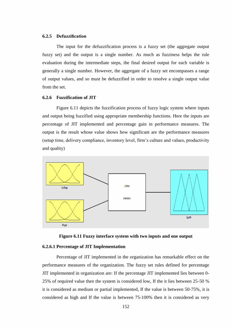
6.2.6 Fuzzification of JIT

Figure 6.11 depicts the fuzzification process of fuzzy logic system where inputs

and output being fuzzified using appropriate membership functions. Here the inputs are

percentage of JIT implemented and percentage gain in performance measures. The

output is the result whose value shows how significant are the performance measures

(setup time, delivery compliance, inventory level, firm’s culture and values, productivity

and quality)

Figure 6.11 Fuzzy interface system with two inputs and one output

6.2.6.1 Percentage of JIT Implementation

Percentage of JIT implemented in the organization has remarkable effect on the

performance measures of the organization. The fuzzy set rules defined for percentage

JIT implemented in organization are: If the percentage JIT implemented lies between 0-

25% of required value then the system is considered low, If the it lies between 25-50 %

it is considered as medium or partial implemented, If the value is between 50-75%, it is

considered as high and If the value is between 75-100% then it is considered as very

153

high or fully implemented as shown in Table 6.1 and the transfer function in fuzzy

format is shown in Figure 6.12.

Table 6.1 Range of Percentage JIT Implemented

Fuzzy Linguistic Term Range

1 Low 0-25%

2 Medium 25-50%

3 High 50-75%

4 Very High 75-100%

Figure 6.12 Transfer function in fuzzy format of Percentage JIT Implemented

6.2.6.2 Gain in Performance Measure

Performance measure is the gains achieved by the organization due to

implementation of JIT. The fuzzy set rules defined for gain in performance measure is

set as: if performance measure lies between 0-10% than it is considered as marginal gain

whereas if gain is greater than 40% than it is considered as extremely high gain. The

actual division of gain in performance measure is given in Table 6.2. The transfer

function in fuzzy format is shown in Figure 6.13.

154

Table 6.2 Range of percentage Gain in Performance Measure

Fuzzy Linguistic Term Range

1 Marginal Gain 0-10%

2 Reasonable Gain 10-25%

3 High Gain 25-40%

4 Extremely Very High >40%

Figure 6.13 Transfer function in fuzzy format of percentage gain in performance

measure

6.2.6.3 Performance Measures

Performance measures are considered as key elements in determining whether or

not an improvement effort in the organization will succeed. Lack of an appropriate

performance measurement system could also impede a successful JIT implementation.

There are many performance measures that from which an organization can reap its

goals. Most critical performance measures which effects the performance of the

organization are setup time (ST), delivery compliance (DC), inventory level (IL), firm’s

culture and values (FCV), productivity (P) and quality (Q). These performance

measures are divided according to weightage gained from the feedback response from

155

various organizations. These weigh age are shown in Table 6.3 and transfer function in

fuzzy format is shown in Figure 6.14.

Table 6.3 Percent Weightage of Performance Measure

Fuzzy Performance Measure Range

1 Setup- Time (ST) 0-25%

2 Delivery Compliance (DC) 0-40%

3 Inventory Level (IL) 10-40%

4 Firm’s Culture and Values (FCV) 25-35%

5 Productivity (P) 25-40%

6 Quality (Q) >25%

Figure 6.14 Transfer function in fuzzy format of percent weightage of performance

measure

6.2.7 Rule Evaluation in Fuzzy

The rule evaluation in fuzzy logic is a platform on which relation between input

and output is made. In this system inputs are expert rule, and fuzzy input obtained from

the first step, while output is fuzzy value of significant performance measures. In this

study, there are two variables, percentage JIT implemented and percentage gain in

156

performance measure and each has four subdivisions. So at least sixteen (4×4) rules to

describe this model are needed. These rules are based on statement of if-then and are

formed with data knowledge and guidance given by expert in a manufacturing company.

If –then statement has a form of ―If A is X then B is Y. Notice that the above actions

are not crisp, and can be change according to the environment of each industry. The

objective is to present a frame work for developing rule for the fuzzy controller. A

summary of the application of each action in fuzzy logic (using Matlab) is shown in

Figure 6.15.

Figure 6.15 Fuzzy set rules for performance measures.

Figure 6.16 Rule Viewer for JIT- Result

157

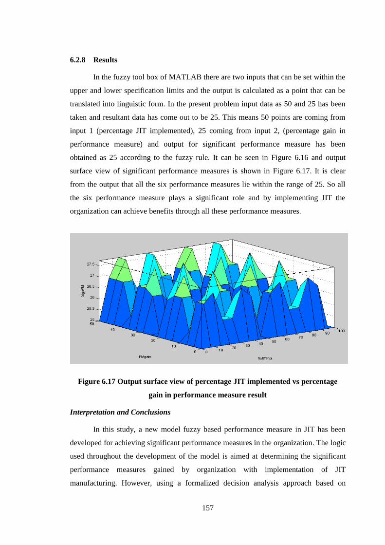
6.2.8 Results

In the fuzzy tool box of MATLAB there are two inputs that can be set within the

upper and lower specification limits and the output is calculated as a point that can be

translated into linguistic form. In the present problem input data as 50 and 25 has been

taken and resultant data has come out to be 25. This means 50 points are coming from

input 1 (percentage JIT implemented), 25 coming from input 2, (percentage gain in

performance measure) and output for significant performance measure has been

obtained as 25 according to the fuzzy rule. It can be seen in Figure 6.16 and output

surface view of significant performance measures is shown in Figure 6.17. It is clear

from the output that all the six performance measures lie within the range of 25. So all

the six performance measure plays a significant role and by implementing JIT the

organization can achieve benefits through all these performance measures.

Figure 6.17 Output surface view of percentage JIT implemented vs percentage

gain in performance measure result

Interpretation and Conclusions

In this study, a new model fuzzy based performance measure in JIT has been

developed for achieving significant performance measures in the organization. The logic

used throughout the development of the model is aimed at determining the significant

performance measures gained by organization with implementation of JIT

manufacturing. However, using a formalized decision analysis approach based on

158

multiple criteria and rule-based system is the contribution of the presented model. One

of the main advantages of proposed model is that it enhances the decision making

capacity of organizations which are at different stages of implementation of JIT or

planning to implement JIT. The model can be used to understand, describe, analyze and

prescribe the significant performance measure, from which the organization can gain

benefits by implementing JIT.

Some of the salient features of the proposed model include

Enhancement is decision making capacity of organization that are at various

stages of JIT implementation.

Better understanding, describing, analyzing and prescribing the performance

measures the organization can achieve by implementing JIT.

6.3 Validation of JIT performance measure model through Structural Equation

Modeling

6.3.1 Use of Structural Equation Modeling in Manufacturing Industry

A number of serious difficulties have been posed by modeling of industrial

production process. This is because that large number of independent variables is

involved and they have great impact on the performance measures or dependent

variables. Moreover the independent variable also interacts with each other, whereby

traditional methods are not viable and more approximations are required to successfully

model the production process.

All these difficulties were noted by many authors in early times by Wright

(1932). In the year 1970’s, conceptual theoretical framework called SEM was developed

with purpose of finding relationship between independent and dependent variable. After

that some authors also applied SEM in this research work. Vinodh and Dino (2012)

applied SEM model for sustainable manufacturing practices and the purpose of their

research study was to study the sustainable manufacturing practices across industrial

sectors and to identify the critical factors for its success implementation. Lin et al.

(2005) have applied SEM in supply chain management. Wu and LI (2010) also applied

structural equation model in location selection and spatial layout of convention and

convention and exhibition industry cluster. Tan (2001) applier SEM for new product

design and development. In the research author uses structural equation modeling to

159

analyze the effects of supplier assessment, Just-In-Time, and quality management

strategies on new product design and development.

Although SEM has been used by many authors in their research work for certain

purpose, the application of SEM in modeling the manufacturing environment is

attempted by very few authors which formed the research problem. Review of literature

indicated that there are no concrete evidence of use of SEM in manufacturing industry

particularly for JIT environment, which must be practically feasible in the industry. This

study validates the model developed in Fuzzy logic by using the data collected from

various manufacturing industries implementing JIT.

6.3.2 Variable used in Study

Input / Independent Variables used in the study

With reference to the fuzzy model shown in Fig 6.11 in which percentage of JIT

implemented in an organization and percentage gain in performance measures due to

implementation of JIT issues in the organization were taken. In the preset study one

variable regarding percentage JIT implemented and three factors regarding JIT issues

that leads to gain in performance measure in the organization have been taken. The

input variables selected are shown in Table 6.4:

Table 6.4 Input Variables used in the study

Symbol Name of Variable

Z1 JIT implementation in an organization

Z2 Organization culture, Management Commitment, Employee’s

Involvement and Work Place Organization

Z3 JIT Purchasing

Z4 Production System, Process Control, Daily Schedule Adherence,

Maintenance, Customer’s Orientation

Output / Dependent Variables used in Study

Further, in the fuzzy model six performance measures (PM), Setup- Time (ST),

Delivery Compliance (DC), Inventory Level (IL), Firm’s Culture and Values (FCV),

Productivity (P), Quality (Q) were taken. In this study the performance measure (PM) is

taken as dependent variables. The abbreviations used for performance measure are listed

in Table 6.5.

160

Table 6.5 Symbols used in output variables

Symbol used Name of Output Variable

B11, B12 Setup- Time (ST)

B21, B22 Delivery Compliance (DC)

B31, B32 Inventory Level (IL)

B41, B42 Firm’s Culture and Values (FCV)

B51, B52 Productivity (P)

B61, B62 Quality (Q)

6.3.3 Generating Structural Equation Modeling (SEM) of fuzzy model

‘Figure 6.18 shows the theoretical framework of the JIT model. The key data

required for the SEM model has been obtained from the questionnaires developed for

the study. The questionnaire used includes JIT implementation issues and performance

measures gained by an organization due to implementation of JIT. In the questionnaire 4

point likert scale is used to extract the respondent’s options.

Figure 6.18 Theoretical Model of SEM-JIT

6.3.3.1 Preliminary Analyses

After collection of data various data examination techniques like skewness,

kurtosis, normality test, test for reliability and factor analysis tests were applied. After

applying all the reliability tests data is used to build SEM-JIT model using the AMOS

161

software and the inter-relationship among the variables is established. The values of

skewness <± 2 and kurtosis < ± 7 are considered as acceptable according to Currie et al.

(1999). The Table 6.6 shows the measures of descriptive statistics of all items for

independent variable and dependent variable of model. Since the measures of kurtosis

and skewness for all items are within the range thus it is assumed that the distribution of

data is normal (Figure 6.19).

.

Figure 6.19 Illustration of kurtosis and Skewness

Table 6.6 Values of Skewness and Kurtosis for variable of JIT model

Variables Items

N Minimu

m

Maxim

um Mean Std. Skewness Kurtosis

Statistic Statistic Statistic Statistic Statistic Statistic Std. Error Statistic Std. Error

X1 60 1 4 3.00 .736 -.527 .309 -.413 .608

Z1 X2 60 1 4 2.93 .899 -.155 .309 -1..180 .608

X3 60 1 4 2.92 .944 -.330 .309 -.949 .608

X4 60 1 4 2.73 1.006 -.466 .309 -.791 .608

A11 60 1 4 3.27 .861 -.883 .309 -.177 .608

A12 60 1 4 3.33 .752 -1.138 .309 1.413 .608

Z2 A13 60 1 4 3.12 .825 -.411 .309 -.900 .608

A14 60 2 4 3.03 .663 -.036 .309 -.643 .608

A15 60 1 4 2.70 .926 -.416 .309 -.567 .608

A16 60 1 4 2.85 1.055 -.497 .309 -.944 .608

A17 60 1 4 3.07 1.006 -.963 .309 -.059 .608

162

A18 60 1 4 2.93 .989 -.515 .309 -.790 .608

A21 60 2 4 3.33 .601 -.287 .309 -.607 .608

A22 60 2 4 3.70 .561 -1.747 .309 2.185 .608

A23 60 1 4 3.23 .890 -.932 .309 -.003 .608

Z3 A24 60 2 4 3.63 .637 -1.542 .309 1.208 .608

A25 60 1 4 3.08 .869 -.806 .309 .167 .608

A26 60 2 4 3.15 .732 -.243 .309 -1.075 .608

A27 60 1 4 3.25 .914 -.802 .309 -.650 .608

A28 60 1 4 3.42 .869 -1.256 .309 .430 .608

Z4

A31 60 1 4 3.22 .555 -.556 .309 3.252 .608

A32 60 1 4 3.22 .846 -1.132 .309 1.056 .608

A33 60 1 4 3.33 .681 -.865 .309 1.018 .608

A34 60 1 4 2.88 .846 -.120 .309 -.897 .608

A35 60 1 4 3.07 .778 -1.011 .309 1.460 .608

A36 60 1 4 2.92 1.013 -.637 .309 -.634 .608

A37 60 2 4 3.48 .651 -.891 .309 -.252 .608

A38 60 1 4 3.17 .785 -.524 .309 -.510 .608

A39 60 2 4 3.30 .788 -.594 .309 -1.129 .608

A310 60 1 4 3.25 .856 -.849 .309 -.193 .608

A311 60 1 4 3.10 .817 -.382 .309 -.871 .608

A312 60 1 4 3.08 .926 -.435 .309 -1.131 .608

PM

B11 60 2 4 3.22 .691 -.315 .309 -.851 .608

B12 60 2 4 3.18 .624 -.145 .309 -.467 .608

B21 60 1 4 3.00 .736 -.263 .309 -.352 .608

B22 60 1 4 2.82 .770 -.591 .309 .395 .608

B31 60 1 4 2.98 .792 -.182 .309 -.838 .608

B32 60 1 4 3.18 .792 -.555 .309 -.533 .608

B41 60 1 4 2.77 .890 .037 .309 -1.007 .608

B42 60 1 4 2.63 .882 -.115 .309 -.644 .608

B51 60 1 4 2.87 .769 .004 .309 -.787 .608

B52 60 1 4 2.53 .892 .193 .309 -.716 .608

B61 60 1 4 3.28 .804 -.769 .309 -.377 .608

B62 60 1 4 3.13 .833 -.622 .309 -.330 .608

163

6.3.3.2 Confirmatory Factor Analysis (CFA)

To see if the data collected is suitable for the study confirmatory factor analysis

have been applied. In the confirmatory factor analysis, the strength of the inter-

correlations among the items was checked by Bartlett’s test of sphericity. The adequacy

of the sample size has been checked by Kaiser Meyer Olkin (KMO) test. In the KMO

test the CFA should be considered appropriate if Barletts test of sphericity is significant

at p <0.05 for CFA, and KMO index should range from 0 to1, with 0.5 as minimum

value for CFA (Tabachnick and Fidell, 2007). The KMO and Bartlett’s Test for the

independent and dependent variable are shown in the Table 6.7 and the values of the test

recommended that the data is suitable to continue with a confirmatory factor analysis

procedure. CFA for all independent and dependent variables of the model are shown in

figures 6.20 to 6.24.

Figure 6.20 Path Diagram of CFA for JIT Implementation issue Z1

Figure 6.21 Path Diagram of CFA for JIT issue Z2

164

Fig. 6.22 Path Diagram of CFA for JIT issue Z3

Figure 6.23 Path Diagram of CFA for JIT issue Z4

Figure 6.24 Path Diagram of CFA for JIT Performance Measure

165

Table 6.7 KMO and Bartlett’s Test for the independent and dependent variables

Variable Kaiser-Meyer-

Olkin Measure Bartlett's Test of Sphericity

Chi-Square value P-value

Z1 0.756 81.100 0.000

Z2 0.744 196.009 0.000

Z3 0.693 109.702 0.000

Z4 0.808 142.283 0.000

Performance Measure

(PM) 0.894 445.850 0.000

If the regression weights are less than 0.5 than that should be removed as they

may cause the SEM model unfit (Rakowski et al., 1997). So in the Figures 6.20 to 6.24

it is seen that in Z1 all the four items have value more than 0.6, in input variable Z2 item

A11 is having value 0.42 so it is deleted, in Z2 item A21, A22 got deleted and in Z4

again six variables got deleted. Then reliability test of the data is done by using

Cronbach’s Alpha and values of chronbach’s Alpha are shown in Table 6.8. The

reliability values more than 0.7 and considered as acceptable vales in chronbach alpha

(Nunally, 1978). From the Table 6.8 it is seen that all the values are more than 0.7 so

data is considered as reliable.

Table 6.8 Cronbach’s Alpha for variables of JIT model

Variables Items Cronbach’s Alpha (α)

Z1 4 .809

Z2 7 .886

Z3 6 .760

Z4 6 .842

Performance Measure (PM) 12 .929

166

6.3.3.3 SEM- JIT Model generation and Result Analysis

Figure 6.25 describes the SEM-JIT model which is constructed using AMOS

20.0 to build up the relationship between each variable in the study. The SEM- JIT

model presents the regression coefficients linking the construct in the study. AMOS

output for un standardized model provides the covariance between independent

variables, the ordinary regression coefficient, the error measurement of each

independent variables and the significance level (p-value) for each relationship.

Figure 6.25 Model 1: describes the full SEM-JIT model

The Path Diagram with the regression coefficients among the construct of SEM-

JIT model is shown in Figure 6.25. The output of model 1 was studied and then

compared with the cut-off criteria given by (Schreiber et al. 2006) for Several Fit

Indexes as shown in Table 6.10. It has been seen that the value of RMR is 0.067. RMR

(root mean square residual) is the square root of the average squared amount by which

167

the sample variances and covariance’s differ from their estimates which is preferred as

he smaller the RMR is the better.

The value of GFI suggested by Jeong and Phillips, (2001) is found to be 0.557.

Although GFI is an alternative to the chi-square test and calculates the proportion of

variances that is accounted by estimating population covariance. The value of AGFI is

0.490 which is based upon degrees of freedom with more saturated models reducing fit

(Tabachnick and Fidell, 2007). The values of GFI and AGFI closer to 0.95 is considered

as a perfect fit of the Model.

6.3.3.4 Modification Indices of SEM- JIT model

The SEM-JIT model1 is modified using the modification indices of AMOS 20.0

as shown in Table 6.9. Modification indices indicate the improvement in fit that may

result in the inclusion of a particular relationship in the model. Instead of showing all

possible modifications, setting a threshold for modification indices reduces the display

of modification indices to a smaller set. Or we can say that the modification index for a

parameter is an estimate of the amount by which the discrepancy function would

decrease if the analysis were repeated with the removed constraints on that parameter.

The actual decrease that would occur may be much more. Each time Amos displays a

modification index for a parameter, it also displays an estimate of the amount by which

the parameter would change from its current constrained value, if the constraints on it

are removed. The modified SEM-JIT model and its output is shown in Figure 6.26.

Table 6.9 Modification Indices for SEM-JIT model

Covariance’s of items M.I. Par Change

e12 <--> e19 11.323 .214

e16 <--> e28 10.415 .213

e9 <--> e12 7.664 .202

Regression Weights of the items M.I. Par Change

A34 <--- Z2 9.025 .327

A34 <--- Z1 4.995 .257

A34 <--- PM 5.460 .399

A25 <--- Z2 5.578 -.197

A26 <--- Z2 9.040 .256

168

Figure 6.26 Model 2: Path diagram of SEM- JIT model after modification

Model Fit summary has been made in Table 6.9 showing the indices before and

after modification. It was seen that after modifying the model 1, there has been slight

improvement in the model 2 as the value of RMR decreased to 0.061. Similarly, the

value of GFI increased to 0.590. The RMSEA value is coming closer to.08 showing a

near model fit. The other values as shown in Table 6.10 are also coming closer to model

fit values like CFI, NFI, and RFI etc.

169

Table 6.10 SEM-JIT model Statistics

Model Fit Summary

Before

Modification

Indices

After

Modification

Indices

Recommended

value for Model

Fit*

CMIN/Df 1.884 1.757 x2/ df < 3.0

Degrees of Freedom 517 509 Smaller is better

Probability level 0.000 0.000

Root-Mean-Square Residual

Index (RMR) 0.067 0.061

Smaller is better;

0 indicates

perfect fit

Root-Mean-Square Error of

Approximation (RMSEA) 0.122 0.113 < 0.08

Baseline Comparisons

Goodness-of-Fit Index (GFI) 0.557 0.590 > 0.95

Adjusted Goodness-of-Fit

Index (AGFI) 0.490 0.520 > 0.95

Comparative Fit Index (CFI) 0.704 0.751 > 0.95

Incremental Fit Index (IFI) 0.712 0.759 > 0.95

Normed Fit Index (NFI) 0.538 0.575 > 0.95

Relative Fit Index (RFI) 0.498 0.532 > 0.95

Tucker-Lewis index (TLI) 0.679 0.725 > 0.95

170

Interpretation and Conclusions

JIT has been employed by many manufacturing organizations in India to

enhance the performance of an organization. Based on the concept of finding out the

significant performance measures a empirical study was done and a JIT model was

developed by using Fuzzy Logic Toolbox of MATLAB which provided the steps for

designing fuzzy interface system using graphical tools (Amin and Karim, 2013). By

implementing that model it was concluded that if the organization implement JIT, all

these performance measure Setup- Time (ST), Delivery Compliance (DC), Inventory

Level (IL), Firm’s Culture and Values (FCV), Productivity (P), Quality (Q) can be

achieved by the organization.

Above study is validated in the present study. In this study SEM-JIT model is

formed with SEM using AMOSE software. Various significant factors used for SEM

model are customer orientation, process control, continuous improvement and business

performance. Further various data examination techniques like test for skewness and

kurtosis i.e. to check the normality of the independent and dependent variables data

have been applied. Through CFA, various items affecting the model to unfit have been

removed from independent and dependent variables. Then using AMOS 20.0 software

Structural Equation Modeling has been performed and statistics data before and after

modification indices were compared. SEM-JIT model implies that companies

implementing the JIT can reap the benefits of performance measures.

6.4 Analytical Hierarchy Process for justification of JIT implementations in

Indian manufacturing industries

6.4.1 Description of structure of model

A detailed analysis of the problem is done for the identification of the important

attributes (sub-objectives) involved in Just in Time manufacturing. For this study, the

selection of attributes has been determined by analysing literatures, from questionnaire

and holding discussions with experts during visits to various industries. The attributes

and the used in the AHP model for the justification of success of JIT are shown in

Figure 6.27.

171

Figure 6.27 Description of Attributes

Alternatives: The alternative system is failure of Just in Time manufacturing in

Indian manufacturing industry. This alternative is compared and evaluated in the light of

above discussed set of attributes.

6.4.2 Formulation of Hierarchy

The schematic hierarchy for decision-making in AHP is formulated by breaking

down the current problem statement into a schematic hierarchy (levels) of decision

attributes as shown in Figure 6.28. In this way we have zeroed down on nine attributes

(OCMC, EIC, JP, PPCFL, KAN, ST, QL, DSAT, CO) and there are two alternatives

(success and failure).

172

Figure 6.28 Schematic Hierarchy formulation of AHP Model

6.4.3 Comparison scale used for pair-wise comparison of attributes

The key step in an AHP model has been Pair-wise comparison, to determine

priority weights of factors and it also provides a rating for alternatives based on

qualitative factors. The AHP model focuses on two factors at a time and determines

their relation to each other, so decision-making will be more easy as to offer relative

(rather than absolute) preference information. The importance of each factor relative to

other is rated by a measurement scale to provide numerical judgments’ corresponding to

verbal judgments’. The discrete scale, from 1 to 9 has been used in this research where 1

represents the equal importance of two factors and 9 represents the highest possible

importance of the factor over another factor, as shown in Figure 6.29.

173

Figure 6.29 Comparison scale used

In the first stage data was collected from various organizations implementing JIT by

distributing questionnaires and then the selected attributes were compare to each other.

In this comparison, the importance of ith sub-objective is compared with jth sub

objective where ith sub-object is represented in row and jth sub- object represents

column. To obtain this, the number of attributes is selected and in our case it is 9. A 9 ×

9 matrix was formed and to fill this matrix following procedure was adopted.

1. The diagonal elements of the matrix always remain 1.

2. Upper triangular matrixes were filled as per the data obtained through

companies and this represents how much one attribute is important than the

other. According to importance of attribute value of each attribute has been

given from 1-9 in Table 6.11.

3. To fill the lower triangular matrix, reciprocal values of the upper diagonal was

used, i.e. if aij is the element of row ith and column jth of the matrix, then the

lower diagonal is filled using this formula aji = 1/aij. Thus, the pair-wise

comparison of matrix for different attributes is shown in Table 6.11.

174

Table 6.11 Comparison matrix pair-wise

OCMC EIC JP PPCFL KAN ST QL DSAT CO

OCMC 1 4 2 5 3 6 3 4 9

EIC 1/4 1 1 4 3 1 4 2 8

JP 1/2 1 1 1 2 3 4 4 6

PPCFL 1/5 1/4 1 1 4 2 3 3 7

KAN 1/3 1/3 1/2 1/4 1 3 4 3 5

ST 1/6 1 1/3 1/2 1/3 1 1 2 6

QL 1/3 1/4 1/4 1/3 1/4 1 1 0.5 4

DSAT 1/4 1/2 1/4 1/3 1/3 1/2 2 1 3

CO 1/9 1/8 1/6 1/7 1/5 1/6 1/4 1/3 1

Sum 3.147 8.459 6.501 12.561 15.118 17.667 22.25 19.834 49

6.4.4. Normalisation of comparison matrix

Having made all the pair wise comparisons and entered the data, the consistency

is determined using the eigen value. So next step is to calculate priority vector that is the

normalised eigenvector of the matrix. For this, each entry in column is divided by the

sum of all entries in that column to get value of normalised matrix. Thus, in each

column we get the sum 1 as shown in Table 6.12.

Table 6.12 Normalised matrix of different variables along with priority weights

OCMC EIC JP PPCFL KAN ST QL DSAT CO Weights

OCMC 0.318 0.473 0.308 0.398 0.198 0.340 0.135 0.201 0.184 0.300

EIC 0.079 0.118 0.154 0.318 0.198 0.057 0.180 0.100 0.163 0.163

JP 0.159 0.118 0.154 0.079 0.132 0.170 0.180 0.201 0.122 0.143

PPCFL 0.034 0.029 0.153 0.079 0.264 0.113 0.135 0.151 0.143 0.126

KAN 0.064 0.039 0.077 0.020 0.066 0.170 0.180 0.151 0.102 0.095

ST 0.053 0.118 0.051 0.040 0.022 0.057 0.045 0.100 0.122 0.066

QL 0.063 0.029 0.038 0.026 0.017 0.057 0.045 0.025 0.081 0.044

DSAT 0.079 0.059 0.038 0.026 0.022 0.028 0.090 0.051 0.061 0.048

CO 0.036 0.150 0.026 0.013 0.013 0.009 0.011 0.017 0.020 0.017

Normalized

sum 1.000 1.000 1.000 1.000 1.000 1.000 1.000 1.000 1.000 1.000

175

From the Table 6.12, it is normalized sum of each column comes out to be one

means that matrix is consistent. The normalised value rij is calculated as:

-------- Eq. 6.2

Thus, the approximate priority weight (W1, W2, …, Wj) for each attribute is

obtained as shown in Table 6.12.

--------------- Eq. 6.3

6.4.5 Check for Consistency

The results of pair wise comparisons are filled in positive reciprocal matrices to

calculate the Eigenvector and Eigen value. The consistency of the judgments is

determined by a measure called consistency ratio (C.R.). The consistency ratio is

obtained to filter out the inconsistent judgments, when the value of the consistency

index (C.I.) is greater than 0.1 then all the judgments are found to be consistent and

accepted for analysis. Saaty (1980) has proved that for any reciprocal matrix, the

maximum Eigen value is equal to the size of comparison matrix, and then a measure of

consistency which is called consistency index (CI) as deviation or degree of consistency

was given by him. Considering above relative weight, that would also represent the

Eigen values of criteria, should verify as below:

---------- Eq. 6.4

Where A denotes the pair-wise comparison decision matrix and is the

highest eigen value. Then consistency index (CI), that measures the inconsistencies of

pair-wise comparisons, is calculated as under:

--------- Eq. 6.5

The last ratio which has to be calculated for consistency check is consistency

ratio (CR). Generally, if the value of CR is less than 0.1, than it is judged that data are

consistent and acceptable. The calculation of CR is as under:

176

------------- Eq. 6.6

where random index (RI) depicts the average RI along with the value obtained

by different orders of the pair-wise comparison matrices. The values of this consistency

test obtained from the above formula are given in Table 6.14, whereas Table 6.13 gives

values of constancy index according to size of matrix. In this case, size of matrix is 9X9

so value of RI from Table 6.13 is 1.45.

Table 6.13 Random Consistency Index (RI)

Size of matrix 1 2 3 4 5 6 7 8 9 10

RI 0 0 0.58 0.9 1.12 1.24 1.32 1.42 1.45 1.49

Table 6.14 Results of consistency test

Maximum Eigen Value (λ max) C.I. R.I. C.R.

10.0765 0.135 1.45 0.0931

From the Table 6.14 it is clear that value of CR is 0.0931 that is <1. Therefore, it

is evident from results that data is consistent and acceptable.

6.4.6 Priority weights for alternatives with respect to attribute

The chances of successfully implementing JIT manufacturing techniques in an

organisation are enhance only if attributes (sub-objectives) present are quite strong.

Priority weights have been used for the measurement of the preference of the alternative

(success or failure) with respect to an attribute. Thus, if one attribute is strong in the

organisation, success is more likely to provide by that attribute, as compared to the other

attribute the presence of which is considered to be weak.

For calculating priority weights, the weight evaluation of each attribute is

multiplied in the matrix of evaluation rating by vector of attribute weight and then

adding over the entire attribute. Table 6.15 depicts the summary of the weights of each

177

attribute according to its importance in the organization. So weight of attributes in Table

6.15 is multiplied with weight of each one of nine attribute in Table 6.12.

The prediction of weight for success JIT is calculated as under:

Decision index of success = 0.87 × 0.300 + 0.85 × 0.163 + 0.87 × 0.143 + 0.34 × 0.126

+ 0.84 × 0.095 + 0.87 × 0.066 + 0.75 × 0.044+ 0.84 × 0.048 + 0.85 × 0.017 = 0.791 or

79.1%

Thus decision index of failure = 1 - 0.791 = 0.209 or 20.9%

It is clear from above that the success rate of JIT in the Indian manufacturing

organisations is 79.1% and the failure rate is 20.9%.

Table 6.15 Priority weights for sub-objectives

Success Failure Weight

OCMC Success 1 7 0.87

Failure 1/7 1 0.13

EIC Success 1 6 0.85

Failure 1/6 1 0.25

JP Success 1 7 0.87

Failure 1/7 1 0.13

PPCFL Success 1 1/2 0.34

Failure 2 1 0.66

KAN Success 1 5 0.84

Failure 1/5 1 0.16

ST Success 1 7 0.87

Failure 1/7 1 0.13

QL Success 1 3 0.75

Failure 1/3 1 0.25

DSAT Success 1 5 0.84

Failure 1/5 1 0.16

CO Success 1 6 0.85

Failure 1/6 1 0.15

178

Interpretation and Conclusions

The AHP method has been used in the selection of the best competitive

advantage for manufacturing organization under uncertainty to develop its most critical

competitive advantage in JIT implementation. Also by using the AHP method, this

study is facile to analyse and affirm the important criteria and attributes, for attaining

the overall objective for JIT implementations in Indian manufacturing organisations.

The results obtained by this study are quite significant and promising and shows that

success rate of JIT implementation in Indian manufacturing industry are 79.1% with are

quite significant. Thus, it is evident that using the philosophy of JIT can bring in

remarkable reforms and enhancement in terms of achievement of manufacturing

excellence in industrial organisations. So, the preferences which have been formed

lastly can be useful in many decision-making steps like relocating and utilization of

resources depending upon decisive and operational functions in the organisation.

6.5 SWOT Analysis of JIT

The SWOT analysis involves systematic thinking and comprehensive

diagnosis of factors relating to a new product, technology, management, or planning

(Weihrich, 1982). It is used extensively in strategic planning, where all factors

influencing the operational environment are diagnosed in great detail (Kotler, 1994).

Specifically, SWOT (Figure 6.30) allows analysts to categorize factors into internal

(strengths, weaknesses) or external (opportunities, threats) as they relate to a decision,

enabling comparison of opportunities and threats with strengths and weaknesses,

respectively. One of the main limitations of this approach, however, is that the

importance of each factor in decision-making cannot be measured quantitatively, and it

is difficult to assess which factor has the greatest influence on the strategic decision

(Pesonon, et al., 2001) Improve the usability of SWOT analysis, several attempts have

been made to expand SWOT with quantitative methods recently (Arslan and Deha,

2008; Amin et al., 2011). The SWOT analysis of JIT has been depicted in Table 6.16.

179

Figure 6.30 SWOT analysis example

Table 6.16 SWOT Analysis of JIT

Strengths Weaknesses

Just-in-time manufacturing keeps

stock holding costs to a bare

minimum. The release of storage

space results in better utilization of

space and thereby bears a favorable

impact on the rent paid and on any

insurance premiums that would

otherwise need to be made.

Just-in-time manufacturing eliminates

waste, as out-of-date or expired

products; do not enter into this

equation at all.

Due to the afore-mentioned low level

of stocks held, the organizations

return on investment (referred to as

ROI, in management parlance) would

generally be high.

Just-in-time manufacturing

provides zero tolerance for

mistakes, as it makes re-working

very difficult in practice, as

inventory is kept to a bare

minimum.

There is a high reliance on

suppliers, whose performance is

generally outside the purview of

the manufacturer.

Due to there being no buffers for

delays, production downtime and

line idling can occur, which

would bear a detrimental effect

on finances and on the

equilibrium of the production

process.

180

Strengths Weaknesses

As under this technique, only

essential stocks are obtained, less

working capital is required, to finance

procurement. Here, a minimum re-

order level is set, and only once that

mark is reached fresh stocks are

ordered, making this a boon to

inventory management too.

As just-in-time production works on a

demand-pull basis, all goods made

would be sold, and thus it

incorporates changes in demand with

surprising ease. This makes it

especially appealing today, where the

market demand is volatile and

somewhat unpredictable.

Just-in-time manufacturing

encourages the right first time

concept, so that inspection costs and

cost of rework is minimized.

High quality products and greater

efficiency can be derived from

following a just-in-time production

system.

Close relationships are fostered along

the production chain under a just-in-

time manufacturing system.

Constant communication with the

customer results in high customer

satisfaction.

Over production is eliminated, when

just-in-time manufacturing is

adopted.

The organization would not be

able to meet an unexpected

increase in orders, due to the fact

that there are no excess finish

goods.

Transaction costs would be

relatively high, as frequent

transactions would be made.

Just-in-time manufacturing may

have certain detrimental effects

on the environment, due to the

frequent deliveries that would

result in increased use of

transportation which in turn

would consume more fossil fuels.

181

Opportunities Threats

Need to remain competitive

globally.

Satisfy global customers.

Eliminate threats faced by

organization from tough

competition, increase of raw

material costs, energy costs and

globalization.

Improve the work culture and

mindset of organization.

To increase the efficiency of the

workers by providing them training,

incentive and to make each worker

multi-skilled.

To improve the quality of product.

To reduce the cost of product.

To ensure that minimum

breakdowns should occur in the

industrial organization.

To ensure that each part is to be

procured or produced as and when

required so as to reduce waste.

Inventory levels and lead time in an

industrial organization should be

reduced to minimum.

There should be optimum utilization

of men, machine and material.

Delay of good due to weather

conditions.

Lack of communication with

suppliers.

Quality of parts delivered by

suppliers.

On time delivery by suppliers.

Attitude of management.

Incentive to workers.

Long working hours for all.

Multi work to be done by workers.

Unions of workers.

Proper training of workers.

Skill level of employee.

Attitude of worker toward work.

Schedule change.

Poor forecasting.

Lack of communication with

customers.

182

Interpretation and Conclusions

The SWOT analysis has been used in the determination of the strengths,

weaknesses, opportunities and threats due to JIT implementation in Indian

manufacturing Industry. By adopting SWOT the organization can analysis its strengths

(characteristics of the business or project that give it an advantage over others),

weaknesses (characteristics that place the team at a disadvantage relative to others),

opportunities (elements that the project could exploit to its advantage) threats (elements

in the environment that could cause trouble for the business or project)

6.7 Concluding Remarks

Indian manufacturing organisations had been facing with various aspects of

changes like complexity of change, competition, customers and creativity from the past

many years. And now in the beginning of the last decade they have well understood that

the strategic implications of various manufacturing methods are very important to

improve competitiveness in business. So in the quest to achieve manufacturing

excellence through improvement initiatives, the leading Indian entrepreneurs have made

sincere efforts to adopt various lean manufacturing initiatives like JIT, TQM, TPM and

TOC as a proactive technique. At the same time they have understand that there is need

to reduce the cost of product with enhance quality.

This chapter presents a strategic JIT for the Indian manufacturing industry for

their sustained growth and competitiveness. Various success factors and obstacles, while

implementing JIT has been highlighted.

Further a new model fuzzy based performance measure in JIT has been

developed for achieving significant performance measures in the organization. This

Fuzzy model is validated by SEM-JIT model, formed with SEM using AMOSE

software. The AHP method has been used in the selection of the best competitive

advantage for manufacturing organization under uncertainty to develop its most critical

competitive advantage in JIT implementation. Lastly SWOT analysis has been

conducted to ascertain strengths, weaknesses, opportunities and threats in JIT

environment.