Chapter - 5 SIMULATION AND IMPLIMENTATION
66
On-Demand Routing In Multi-Hop Wireless Mobile Ad Hoc Networks Simulation and Implementation 73 Chapter - 5 SIMULATION AND IMPLIMENTATION The present research work involves implementing of four routing protocols namely DSDV (Table driven), DSR, AODV and AOMDV (On-demand), and the comprehensive analysis of unipath on demand routing protocols like DSR, AODV and multipath on-demand routing protocol like AOMDV using NS-2 ( version NS- 2.31 ) simulator. We have further compared on-demand routing protocols with one of the efficient table driven routing protocol DSDV to demonstrate that how and why on-demand protocols work better than table driven protocols under the identical conditions of traffic load and mobility pattern. The protocols were also studied under random mobility patterns. The simulation environment, implementation and response are presented in a comprehensive manner, in the section to follow. 5.1 SIMULATION ENVIRONMENT A number of network simulators are available and practiced. Some of the more popular ones are NS-2, GloMoSim [112] , CSIM [113] and OPNET [114] , as highlighted in the table 5.1. The entire simulations were carried out using NS-2.31 network simulator which is a discrete event driven simulator developed at UC Berkeley [20] as a part of the VINT project. The prime goal of NS-2 is to support Research and Education in networking [115] . It is suitable for designing new protocols, comparing different protocols and traffic evaluations. NS-2 simulator developed as collaborative environment of networks is distributed as open source software. Large number of Institutes and Researchers use it as network simulator tool for prototype of network simulation in research studies.
Transcript of Chapter - 5 SIMULATION AND IMPLIMENTATION

On-Demand Routing In Multi-Hop Wireless Mobile Ad Hoc Networks
Simulation and Implementation 73
Chapter - 5
SIMULATION AND IMPLIMENTATION
The present research work involves implementing of four routing protocols
namely DSDV (Table driven), DSR, AODV and AOMDV (On-demand), and the
comprehensive analysis of unipath on demand routing protocols like DSR, AODV
and multipath on-demand routing protocol like AOMDV using NS-2 ( version NS-
2.31 ) simulator. We have further compared on-demand routing protocols with one of
the efficient table driven routing protocol DSDV to demonstrate that how and why
on-demand protocols work better than table driven protocols under the identical
conditions of traffic load and mobility pattern. The protocols were also studied under
random mobility patterns. The simulation environment, implementation and response
are presented in a comprehensive manner, in the section to follow.
5.1 SIMULATION ENVIRONMENT
A number of network simulators are available and practiced. Some of the
more popular ones are NS-2, GloMoSim [112], CSIM [113] and OPNET [114], as
highlighted in the table 5.1.
The entire simulations were carried out using NS-2.31 network simulator
which is a discrete event driven simulator developed at UC Berkeley [20] as a part of
the VINT project. The prime goal of NS-2 is to support Research and Education in
networking [115]. It is suitable for designing new protocols, comparing different
protocols and traffic evaluations.
NS-2 simulator developed as collaborative environment of networks is
distributed as open source software. Large number of Institutes and Researchers use it
as network simulator tool for prototype of network simulation in research studies.
On-Demand Routing In Multi-Hop Wireless Mobile Ad Hoc Networks
Simulation and Implementation 74
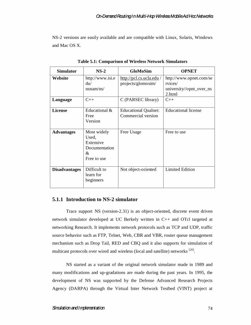
NS-2 versions are easily available and are compatible with Linux, Solaris, Windows
and Mac OS X.
Table 5.1: Comparison of Wireless Network Simulators
Simulator NS-2 GloMoSim OPNET
Website http://www.isi.edu/nsnam/ns/
http://pcl.cs.ucla.edu / projects/glomosim/
http://www.opnet.com/services/ university//opnt_over_ns2.html
Language C++ C (PARSEC library) C++
License Educational & FreeVersion
Educational Qualnet: Commercial version
Educational license
Advantages Most widely Used,ExtensiveDocumentation &Free to use
Free Usage Free to use
Disadvantages Difficult to learn for beginners
Not object-oriented Limited Edition
5.1.1 Introduction to NS-2 simulator
Trace support NS (version-2.31) is an object-oriented, discrete event driven
network simulator developed at UC Berkely written in C++ and OTcl targeted at
networking Research. It implements network protocols such as TCP and UDP, traffic
source behavior such as FTP, Telnet, Web, CBR and VBR, router queue management
mechanism such as Drop Tail, RED and CBQ and it also supports for simulation of
multicast protocols over wired and wireless (local and satellite) networks [20].
NS started as a variant of the original network simulator made in 1989 and
many modifications and up-gradations are made during the past years. In 1995, the
development of NS was supported by the Defense Advanced Research Projects
Agency (DARPA) through the Virtual Inter Network Testbed (VINT) project at

On-Demand Routing In Multi-Hop Wireless Mobile Ad Hoc Networks
Simulation and Implementation 75
Xerox Palo Alto Research Center (PARC), and at the Information Sciences Institute
(USC/ISI) of the University of Southern California. Currently, NS-2 development is
supported through DARPA with Simulation Augmented by Measurement and
Analysis for Networks (SAMAN) and National Science Foundation (NSF) with
Collaborative Simulation for Education and Research (CONSER), in collaboration
with other researchers including the ICSI [115] (International Computer Science
Institute) and Center for Internet Research (ICIR).
5.1.2 Operating System and Installation of NS-2
NS-2 can run under the environment of both UNIX and Windows operating
systems. The user can choose to install it partly or completely, however many
supporting components are desirable during installation for successful running of NS
simulation. For beginners it is suggested to make a complete installation that
automatically installs all necessary components at once and it requires about 320 MB
disk space. With the higher degree of familiarization and expertise the user can go for
partial installation of NS-2, for the faster simulation.
When operated under Windows, a piece of software called Cygwin is required
before the installation of NS-2. Cygwin could provide a Linux-like environment under
Windows. During installation of Cygwin, components XFree86-base, XFree86-bin,
XFree86-prog, XFree86-lib, XFree86-etc, make, patch, perl, gcc, gcc-g++, gawk,
gnuplot, tar and gzip must be chosen because they are required by NS-2 installation.
Guidelines for installation of NS-2 under Windows are available in [116].
5.1.3 General Structure and Architecture of NS-2
A simplified user's view is depicted in Fig 5.1[115]. NS-2 is Object-oriented
Tcl (OTcl) script interpreter that has a simulation event scheduler and network
component object libraries, and network setup (plumbing) module libraries. To setup
and run a simulation network, a user should write an OTcl script that initiates an event
scheduler, sets up the network topology using the network objects and the plumbing
functions in the library informing traffic sources to start and stop transmitting packets
through the event scheduler.

On-Demand Routing In Multi-Hop Wireless Mobile Ad Hoc Networks
Simulation and Implementation 76
Another major component of NS-2 beside network objects is the event
scheduler. An event in NS is a packet ID that is unique for a packet with scheduled
time and the pointer to an object that handles the event. In NS, an event scheduler
keeps track of simulation time and fires all the events in the event queue scheduled for
the current time by invoking appropriate network components by an Event Scheduler
which initiate the appropriate action associated with packet pointed by the event.
Fig 5.1: Simplified User's View of NS-2
NS-2 is written not only in OTcl but in C++ also. For efficient operation, NS-2
separates the data path implementation from control path implementations. In order to
reduce packet and event processing time (not simulation time), the event scheduler
and the basic network component objects in the data path are written and compiled
using C++. These compiled objects are made available to the OTcl interpreter through
an OTcl linkage that creates a matching OTcl object for each of the C++ objects and
makes the control functions and the configurable variables specified by the C++
object acting as member functions and member variables of the corresponding OTcl
object. In this way, the controls of the C++ objects are given to OTcl. It is also
possible to add member functions and variables to a C++ linked OTcl object. The
objects in C++ that do not need to be controlled in a simulation or internally used by
OTcl : Tcl interpreterWith OO extension
NS Simulation Library* Event Scheduler Objects* Network Component Objects* Network Setup Helping
Modules (Plumbing Modules)
OTcl ScriptSimulationProgram
SimulationResults
Analysis
NAMNetwork Animator

On-Demand Routing In Multi-Hop Wireless Mobile Ad Hoc Networks
Simulation and Implementation 77
another object do not need to be linked to OTcl. Likewise, an object (not in the data
path) can be entirely implemented in OTcl.
Fig 5.2 shows an object hierarchy in C++ and OTcl. For C++ objects that
have an OTcl linkage forming a hierarchy, there is a matching OTcl object hierarchy
very similar to that of C++.
Fig. 5.2: C++ and OTcl Duality
Fig.5.3: Architectural View of NS-2
OTcl
C++
Event Scheduler
tclcl
otcl
tcl 8.0
NS-2
NetworkComponent

On-Demand Routing In Multi-Hop Wireless Mobile Ad Hoc Networks
Simulation and Implementation 78
Fig 5.3 shows the general architecture of NS-2. A general user (not an NS
developer) can be thought of standing at the left bottom corner, designing and running
simulations in Tcl using the simulator objects in the OTcl library. The event
schedulers and most of the network components are implemented in C++ and
available to OTcl through an OTcl linkage that is implemented using tclcl. The whole
thing together makes NS, which is an Object Oriented extended Tcl Interpreter with
network simulator libraries.
The procedural flow involved in NS-2 simulation programming is as follows-
The user has to program with OTcl script language to initiate an event
scheduler, set up the network topology using the network objects and informs traffic
sources to start and stop transmitting packets through the event scheduler. OTcl script
is executed by NS-2. The simulation results from running this script in NS-2 include
one or more text based output files and an input to a graphical simulation display tool
called Network Animator (NAM). Text based files record the activities taking place in
the network. It can be analyzed by other tools such as ‘Perl’ or ‘Gwak’ to evaluate the
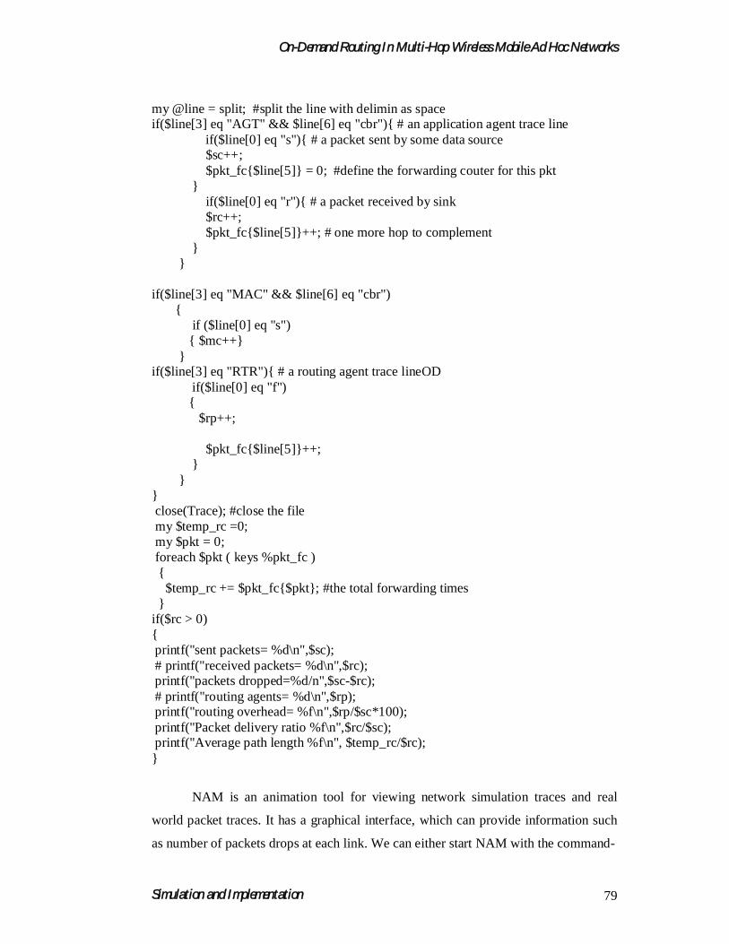
results as illustrated in the ‘Perl’ program as follows.
Perl Program to evaluate the Performance Metrics
#!/usr/bin/perl
use :strict;# to run this programm pass output trace file as command line aurgument
if($#ARGV<0){ printf("Usage: <trace-file>\n"); exit 1;}# to open the given trace fileopen(Trace, $ARGV[0]) or die "Cannot open the trace file";my $sc = 0; # sending countermy $rc = 0; # receiving countermy $rp = 0;my $mc =0;my %pkt_fc = (); #packet forwarding counterwhile(<Trace>){ # read one line in from the file
On-Demand Routing In Multi-Hop Wireless Mobile Ad Hoc Networks
Simulation and Implementation 79
my @line = split; #split the line with delimin as spaceif($line[3] eq "AGT" && $line[6] eq "cbr"){ # an application agent trace line if($line[0] eq "s"){ # a packet sent by some data source
$sc++; $pkt_fc{$line[5]} = 0; #define the forwarding couter for this pkt } if($line[0] eq "r"){ # a packet received by sink $rc++; $pkt_fc{$line[5]}++; # one more hop to complement}
}
if($line[3] eq "MAC" && $line[6] eq "cbr") { if ($line[0] eq "s") { $mc++}
}if($line[3] eq "RTR"){ # a routing agent trace lineOD
if($line[0] eq "f") { $rp++;
$pkt_fc{$line[5]}++;}
}}close(Trace); #close the file my $temp_rc =0;my $pkt = 0;foreach $pkt ( keys %pkt_fc )
{ $temp_rc += $pkt_fc{$pkt}; #the total forwarding times }if($rc > 0){printf("sent packets= %d\n",$sc);# printf("received packets= %d\n",$rc);printf("packets dropped=%d/n",$sc-$rc);# printf("routing agents= %d\n",$rp);printf("routing overhead= %f\n",$rp/$sc*100);printf("Packet delivery ratio %f\n",$rc/$sc);printf("Average path length %f\n", $temp_rc/$rc);}
NAM is an animation tool for viewing network simulation traces and real
world packet traces. It has a graphical interface, which can provide information such
as number of packets drops at each link. We can either start NAM with the command-

On-Demand Routing In Multi-Hop Wireless Mobile Ad Hoc Networks
Simulation and Implementation 80
'nam <nam-file>'
where '<nam-file>' is the name of a NAM trace file that was generated by NS, or one
can execute it directly out of the Tcl simulation script for visualization of node
movement. Fig 5.4 shows the screen shot of a NAM window with important
functions.
Fig 5.4: Screenshot of a Nam Window
5.1.4 The Basic Wireless Model in NS-2
The wireless model essentially consists of the Mobile Node at the core, with
additional supporting features that allows simulations of multi-hop Ad hoc networks,
wireless LANs etc. The Mobile Node object is a split object. The C++ class Mobile
Node is derived from parent class Node. A Mobile Node thus is the basic Node object
with added functionalities of a wireless and mobile node with the ability to move
within a given topology, ability to receive and transmit signals to and from a wireless
On-Demand Routing In Multi-Hop Wireless Mobile Ad Hoc Networks
Simulation and Implementation 81
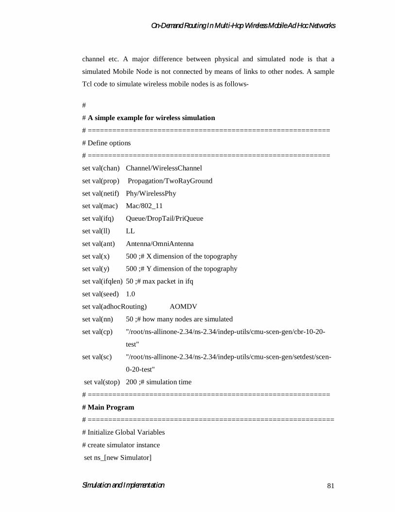
channel etc. A major difference between physical and simulated node is that a
simulated Mobile Node is not connected by means of links to other nodes. A sample
Tcl code to simulate wireless mobile nodes is as follows-
#
# A simple example for wireless simulation
# ===========================================================
# Define options
# ===========================================================
set val(chan) Channel/WirelessChannel
set val(prop) Propagation/TwoRayGround
set val(netif) Phy/WirelessPhy
set val(mac) Mac/802_11
set val(ifq) Queue/DropTail/PriQueue
set val(ll) LL
set val(ant) Antenna/OmniAntenna
set val(x) 500 ;# X dimension of the topography
set val(y) 500 ;# Y dimension of the topography
set val(ifqlen) 50 ;# max packet in ifq
set val(seed) 1.0
set val(adhocRouting) AOMDV
set val(nn) 50 ;# how many nodes are simulated
set val(cp) "/root/ns-allinone-2.34/ns-2.34/indep-utils/cmu-scen-gen/cbr-10-20-
test"
set val(sc) "/root/ns-allinone-2.34/ns-2.34/indep-utils/cmu-scen-gen/setdest/scen-
0-20-test"
set val(stop) 200 ;# simulation time
# ===========================================================
# Main Program
# ============================================================
# Initialize Global Variables
# create simulator instance
set ns_[new Simulator]

On-Demand Routing In Multi-Hop Wireless Mobile Ad Hoc Networks
Simulation and Implementation 82
# setup topography object
set topo [new Topography]
# create trace object for ns and nam
set tracefd [open p0-aomdv.tr w]
set namtrace [open p0-aomdv.nam w]
$ns_ trace-all $tracefd
$ns_ namtrace-all-wireless $namtrace $val(x) $val(y)
# define topology
$topo load_flatgrid $val(x) $val(y)
# Create God
set god_ [create-god $val(nn)]
# define how node should be created
#global node setting
set chan [new $val(chan)]
$ns_ node-config -adhocRouting $val(adhocRouting) \
-llType $val(ll) \
-macType $val(mac) \
-ifqType $val(ifq) \
-ifqLen $val(ifqlen) \
-antType $val(ant) \
-propType $val(prop) \
-phyType $val(netif) \
-channel $chan \
-topoInstance $topo \
-agentTrace ON \
-routerTrace ON \
-macTrace OFF
# Create the specified number of nodes [$val(nn)] and "attach" them
# to the channel.
for {set i 0} {$i < $val(nn) } {incr i} {
On-Demand Routing In Multi-Hop Wireless Mobile Ad Hoc Networks
Simulation and Implementation 83
set node_($i) [$ns_ node]
$node_($i) random-motion 0 ;# disable random motion
}
# Define node movement model
puts "Loading connection pattern..."
source $val(sc)
# Define traffic model
puts "Loading scenario file..."
source $val(cp)
# Define node initial position in nam
for {set i 0} {$i < $val(nn)} {incr i} {
# 20 defines the node size in nam, must adjust it according to your scenario
# The function must be called after mobility model is defined
$ns_ initial_node_pos $node_($i) 20
}
# Tell nodes when the simulation ends
for {set i 0} {$i < $val(nn) } {incr i} {
$ns_ at $val(stop).0 "$node_($i) reset";
}
$ns_ at $val(stop).0002 "puts \"NS EXITING...\" ; $ns_ halt"
puts $tracefd "M 0.0 nn $val(nn) x $val(x) y $val(y) rp $val(adhocRouting)"
puts $tracefd "M 0.0 sc $val(sc) cp $val(cp) seed $val(seed)"
puts $tracefd "M 0.0 prop $val(prop) ant $val(ant)"
puts "Starting Simulation..."
$ns_ run
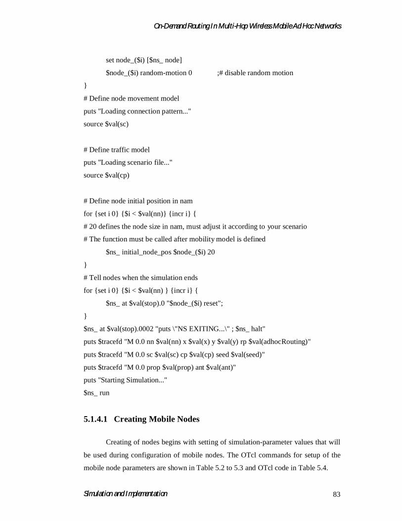
5.1.4.1 Creating Mobile Nodes
Creating of nodes begins with setting of simulation-parameter values that will
be used during configuration of mobile nodes. The OTcl commands for setup of the
mobile node parameters are shown in Table 5.2 to 5.3 and OTcl code in Table 5.4.

On-Demand Routing In Multi-Hop Wireless Mobile Ad Hoc Networks
Simulation and Implementation 84
Table 5.2: Part of the Tcl Script for Setting Mobile Node Parameter
Part of the Tcl script for setting of
parameters
Explanations
set val(chan) Channel/Wireless Channel
set val(prop) Propagation/TwoRayGround
set val(netif) Phy/WirelessPhy
set val(mac) Mac/802_11
set val(ifq) Queue/DropTail/PriQueue
set val(ll) LL
set val(ant) Antenna/OmniAntenna
set val(ifqlen) 50
set val(nn) 50
set val(rp) AOMDV
;# channel type
;# radio-propagation model
;# network interface type
;# MAC type
;# interface queue type
;# link layer type
;# antenna model
;# max packet in ifq
;# number of mobile nodes
;# routing protocol
Table 5.3: Part of the Tcl Script for Configuration of Nodes
$ns_ node-config -adhocRouting $val(rp) \
-llType $val(ll) \
-macType $val(mac) \
-ifqType $val(ifq) \
-ifqLen $val(ifqlen) \
-antType $val(ant) \
-propType $val(prop) \
-phyType $val(netif) \
-channelType $val(chan) \
-topoInstance $topo \
-agentTrace ON \
-routerTrace ON \
-macTrace OFF \
-arpTrace OFF \
-movementTrace OFF
On-Demand Routing In Multi-Hop Wireless Mobile Ad Hoc Networks
Simulation and Implementation 85
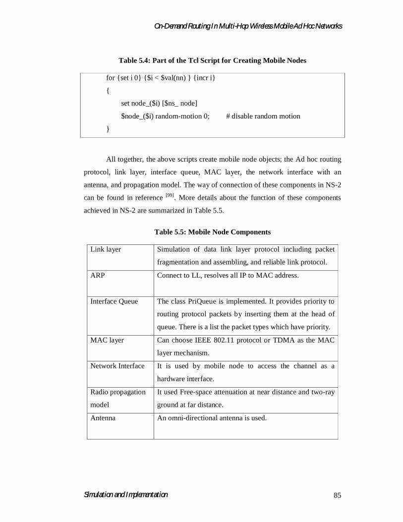
Table 5.4: Part of the Tcl Script for Creating Mobile Nodes
for {set i 0} {$i < $val(nn) } {incr i}
{
set node_($i) [$ns_ node]
$node_($i) random-motion 0; # disable random motion
}
All together, the above scripts create mobile node objects; the Ad hoc routing
protocol, link layer, interface queue, MAC layer, the network interface with an
antenna, and propagation model. The way of connection of these components in NS-2
can be found in reference [99]. More details about the function of these components
achieved in NS-2 are summarized in Table 5.5.
Table 5.5: Mobile Node Components
Link layer Simulation of data link layer protocol including packet
fragmentation and assembling, and reliable link protocol.
ARP Connect to LL, resolves all IP to MAC address.
Interface Queue The class PriQueue is implemented. It provides priority to
routing protocol packets by inserting them at the head of
queue. There is a list the packet types which have priority.
MAC layer Can choose IEEE 802.11 protocol or TDMA as the MAC
layer mechanism.
Network Interface It is used by mobile node to access the channel as a
hardware interface.
Radio propagation
model
It used Free-space attenuation at near distance and two-ray
ground at far distance.
Antenna An omni-directional antenna is used.

On-Demand Routing In Multi-Hop Wireless Mobile Ad Hoc Networks
Simulation and Implementation 86
5.1.4.2 Trace File Formats in Wireless Networks
Trace file is one of the text-based results that the user gets from a simulation.
It records the actions and relevant information of every discrete event in the
simulation. There is variety of forms for trace files. Simulations using different
simulation networks or using different routing protocols could get trace files having
different trace file formats. For example, a wired network and a wireless network
have absolutely different format for recording each event. In the same network, for
example in wireless networks, each routing protocol has its own format of the routing
record. Useful material describing all kinds of record format can be found [117] in
literature. In the trace file, actions of different layers in the network can be traced. It
includes agent trace, router trace, MAC trace and movement trace. All of these traced
events can be written to a file in a predefined format. When the user simulates large
events, the trace file can be very large. It will not only require time to generate the
trace file during simulation but also need space to store that increases exponentially
with number of nodes. As a result, user should always prefer to choose minimum
possible number of parameters to trace. For example, in simulation of Section 5.1.4,
we would always take the agent trace and the router trace in on-mode, while MAC
trace and movement trace in off-mode of a trace function to keep track of actions of
nodes in the routing layer.
A typical CMU trace format for CBR traffic is as follows-
s 20.000000000 _0_ AGT --- 6 cbr 512 [0 0 0 0] ------- [0:0 1:0 32 0]
r 20.000000000 _0_ RTR --- 6 cbr 512 [0 0 0 0] ------- [0:0 1:0 32 0]
s 20.000000000 _0_ RTR --- 6 cbr 532 [0 0 0 0] ------- [0:0 1:0 32 1]
s 20.000275000 _0_ MAC --- 6 cbr 584 [13a 1 0 800] ------- [0:0 1:0 32 1]
r 20.004947063 _1_ MAC --- 6 cbr 532 [13a 1 0 800] ------- [0:0 1:0 32 1]
s 20.004957063 _1_ MAC --- 0 ACK 38 [0 0 0 0]
r 20.004972063 _1_ AGT --- 6 cbr 532 [13a 1 0 800] ------- [0:0 1:0 32 1]
r 20.005261125 _0_ MAC --- 0 ACK 38 [0 0 0 0]

On-Demand Routing In Multi-Hop Wireless Mobile Ad Hoc Networks
Simulation and Implementation 87
The components of format separated by space called field. The first field can
be r, s, f and d for received, send, forward and drop the data packets respectively. The
second field indicates the time of the event occurrence. The third field is the node
number. The fourth field is the trace name that can be AGT, RTR, MAC, and IFQ.
These represents transport, routing, and MAC layer respectively. IFQ indicate events
related to the Interface Priority Queue.
The number after the dashes is a Globally Unique Sequence Number of a
packet. The letters after the number give the traffic type. Traffic types can be CBR
(Constant Bit Rate), TCP (Transport Control Protocol) and ACK. The number right
after the packet type is the packet size in bytes. The following two square brackets
separated by the dashes are MAC and routing layer information such as source and
destination addresses. With the information recorded in each event, performance
metrics such as packet delivery ratio, throughput, packet loss, and end-to-end delay
can be calculated with the help of some additional programs using Gawk, Perl,
Gnuplot , Tracegraph e.t.c.
Interpretation of Trace file format is as follows-
ACTION: [s|r|D]: s -- sent, r -- received, D -- dropped
WHEN: the time when the action happened
WHERE: the node where the action happened
LAYER: AGT -- application,
RTR -- routing,
LL -- link layer (ARP is done here)
IFQ -- outgoing packet queue (between link and mac layer)
MAC -- mac,
PHY -- physical
flags: [......]
SEQNO: the sequence number of the packet
TYPE: the packet type
cbr -- CBR data stream packet
DSR -- DSR routing packet (control packet generated by routing)
RTS -- RTS packet generated by MAC 802.11

On-Demand Routing In Multi-Hop Wireless Mobile Ad Hoc Networks
Simulation and Implementation 88
ARP -- link layer ARP packet
SIZE: the size of packet at current layer, when packet goes down, size increases, goes
up size decreases
[a b c d]: a -- the packet duration in mac layer header
b -- the mac address of destination
c -- the mac address of source
d -- the mac type of the packet body
flags: [......]
[source node ip : port number
destination node ip (-1 means broadcast) : port number
ip header ttl
ip of next hop (0 means node 0 or broadcast)]
Interpretation of sample of trace files as follows-
s 76.000000000 _98_ AGT --- 1812 cbr 32 [0 0 0 0] ---- [98:0 0:0 32 0] -------(5.1)
Trace file (5.1) can be interpreted as follows:
Application 0 (port number) on node 98 sent a CBR packet whose ID is 1812 and size
is 32 bytes, at time 76.0 second, to application 0 on node 0 with TTL is 32 hops. The
next hop is not decided yet.
r 0.010176954 _9_ RTR - 1 gpsr 29 [0 ffffffff 8 800] --- [8:255 -1:255 32 0] --(5.2)
While trace file (5.2) can be interpreted as follows:
As the routing agent on node 9 received a GPSR broadcast (mac address 0xff
and ip address is -1, either of them means broadcast) routing packet whose ID is 1 and
size is 29 bytes, at time 0.010176954 second, from node 8 (both MAC and IP
addresses are 8), port 255 (routing agent).

On-Demand Routing In Multi-Hop Wireless Mobile Ad Hoc Networks
Simulation and Implementation 89
5.1.5 Generating Node-Movement and Traffic-Connection Files for Large Wireless Scenarios
5.1.5.1 Generation of Node Movement
A tool called ‘setdest’ is developed by CMU (Carnegie Mellon University) for
generating random movements of nodes in the wireless network. It defines node
movements with specific moving speed toward a random or specified location within
a fixed area. When the node arrives to the movement location, it could be set to stop
for a period of time. After that, the node keeps on moving towards the next location.
The location ‘setdest’ is at the directory-
‘~ns/indep-utils/cmu-scen-gen/setdest/’
Users need to run ‘setdest’ program before running the simulation program.
The options of ‘setdest’ command and corresponding interpretation are shown in
Table 5.6.
./setdest [-v version ] [-n num_of_nodes] [-p pausetime] [-M maxspeed] [-t simtime]
[-x maxx] [-y maxy] > [outdir/movement-file].
Option details as shown table 5.6.
Table 5.6: Options with ‘Setdest’ Sub-Command
Options Interpretation
-v version Version of simulator used.
-n num Number_ of _nodes total number of node in the scenario
-p pausetime Duration when a node stays still after it arrive a location. If this value is set to 0, it means that the node won’t stop when it arrive a location and keep on moving.
-M maxspeed Maximum moving speed of nodes. Nodes will move at a random speed choosing from the range [0, maxspeed].
-t simtime Simulation time.
-x maxx Maximum length of the area.
-y maxy Maximum width of the area.
On-Demand Routing In Multi-Hop Wireless Mobile Ad Hoc Networks
Simulation and Implementation 90
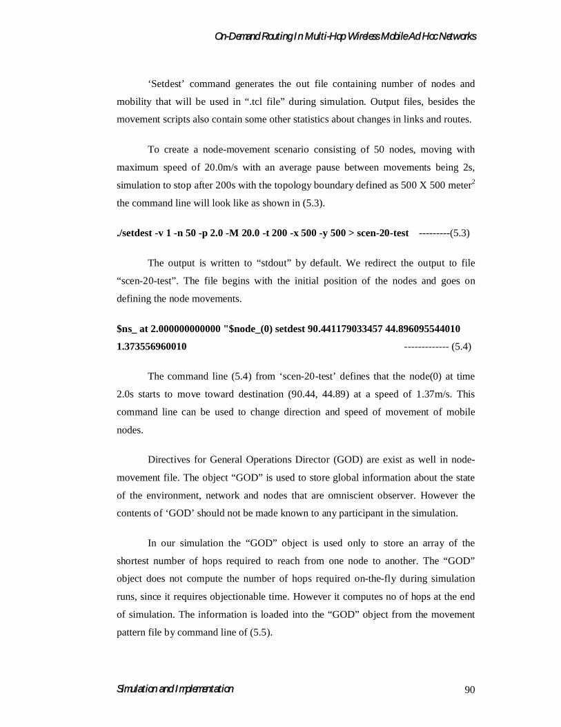
‘Setdest’ command generates the out file containing number of nodes and
mobility that will be used in “.tcl file” during simulation. Output files, besides the
movement scripts also contain some other statistics about changes in links and routes.
To create a node-movement scenario consisting of 50 nodes, moving with
maximum speed of 20.0m/s with an average pause between movements being 2s,
simulation to stop after 200s with the topology boundary defined as 500 X 500 meter2
the command line will look like as shown in (5.3).
./setdest -v 1 -n 50 -p 2.0 -M 20.0 -t 200 -x 500 -y 500 > scen-20-test ---------(5.3)
The output is written to “stdout” by default. We redirect the output to file
“scen-20-test”. The file begins with the initial position of the nodes and goes on
defining the node movements.
$ns_ at 2.000000000000 "$node_(0) setdest 90.441179033457 44.896095544010
1.373556960010 ------------- (5.4)
The command line (5.4) from ‘scen-20-test’ defines that the node(0) at time
2.0s starts to move toward destination (90.44, 44.89) at a speed of 1.37m/s. This
command line can be used to change direction and speed of movement of mobile
nodes.
Directives for General Operations Director (GOD) are exist as well in node-
movement file. The object “GOD” is used to store global information about the state
of the environment, network and nodes that are omniscient observer. However the
contents of ‘GOD’ should not be made known to any participant in the simulation.
In our simulation the “GOD” object is used only to store an array of the
shortest number of hops required to reach from one node to another. The “GOD”
object does not compute the number of hops required on-the-fly during simulation
runs, since it requires objectionable time. However it computes no of hops at the end
of simulation. The information is loaded into the “GOD” object from the movement
pattern file by command line of (5.5).

On-Demand Routing In Multi-Hop Wireless Mobile Ad Hoc Networks
Simulation and Implementation 91
$ns_ at 899.642 "$god_ set-dist 23 46 2" ----------- (5.5)
This implies that the shortest path between node 23 and node 46 changed to 2 hops at
time 899.642 s.
The “setdest” program generates node-movement files using the random waypoint
algorithm. The commands are included in the main program to load these files in the
“GOD” object.
5.1.5.2 Generation of Random Traffic
Random traffic connections of TCP and CBR can be setup between mobile
nodes using a traffic-scenario generator script. To generate random flows of traffic, a
Tcl script called “cbrgen” can be used. This script helps to generate the traffic load.
The load can be either TCP or CBR. These scripts are stored in the file ‘cmu-scen-
gen’ located in the directory-
~ns/indep-utils/cmu-scen-gen
The program “cbrgen.tcl” is used according to the command line (5.6) and
with option is shown in Table 5.7.
ns cbrgen.tcl [-type cbr|tcp] [-nn nodes] [-seed seed] [-mc connections] [-rate
rate] > traffic-file -------- (5.6)
Table 5.7: Option with Cbrgen Sub-Commands
Command Options Interpretation
-type cbr|tcp Type of the generated traffic, TCP or CBR
-nn nodes Total number of nodes
-seed seed Random seed
-mc connections Number of connections
-rate rate Number of packets per second. In CBR, packet
length is fixed as 512 byte during the
simulation.

On-Demand Routing In Multi-Hop Wireless Mobile Ad Hoc Networks
Simulation and Implementation 92
Considering CBR, the data rate can be calculated as follows-
Data Rate (bits/second) = 512 bytes*8 bits/bytes * rate (packets/second defined in
"cbrgen")
The command line (5.7) creates a CBR connection file between 50 nodes, having
maximum of 20 connections, with a seed value of 1.0 and a rate of 4.0.
ns cbrgen.tcl -type cbr -nn 50 -seed 1.0 -mc 20 -rate 4.0 > cbr-20-test --------
(5.7)
From cbr-20-test file (into which the output of the generator is redirected) thus created
one of the cbr connections looks like as follows-
#
# 2 connecting to 3 at time 82.557023746220864
#
set udp_(0) [new Agent/UDP]
$ns_ attach-agent $node_(2) $udp_(0)
set null_(0) [new Agent/Null]
$ns_ attach-agent $node_(3) $null_(0)
set cbr_(0) [new Application/Traffic/CBR]
$cbr_(0) set packetSize_ 512
$cbr_(0) set interval_ 0.25
$cbr_(0) set random_ 1
$cbr_(0) set maxpkts_ 10000
$cbr_(0) attach-agent $udp_(0)
$ns_ connect $udp_(0) $null_(0)
$ns_ at 82.557023746220864 "$cbr_(0) start"
Thus a UDP connection is setup between node 2 and 3. Total UDP sources (chosen
between nodes 0-50) and total number of connections setup is indicated as 20, at the
end of the file cbr-20-test.

On-Demand Routing In Multi-Hop Wireless Mobile Ad Hoc Networks
Simulation and Implementation 93
5.2 IMPLEMENTATION
The performance of Ad hoc network is studied under varying condition of the
traffic load and mobility of nodes. Two models used in the simulation study of
evaluation of on demand and table driven protocols for Ad hoc networks are as
follows-
1. Mobility Generation Model. It is used to study the effect of mobility
of nodes on overall performance of the network.
2. Traffic Generation Model. It is used to study the effect of traffic load
on the network.
Implementation study begins with simulation of Network Environment. This
requires setting of simulation network parameters. These parameters are depicted in
the Table 5.8.
Table 5.8: Simulation Parameters
SerialNo.
Parameters Value
1 Number of nodes 50
2 Simulation Time 200sec.
3 Area 500*500m2
4 Max Speed 20 m/s
5 Traffic Source CBR
6 Pause Time (sec) 0,20,30,40,100
7 Packet Size 512 Bytes
8 Packets Rate 4 Packets/s
9 Max. Number of connections 10,20,30,40
10 Bandwidth 10Mbps
11 Delay 10 ms
12 Mobility model used Random way point

On-Demand Routing In Multi-Hop Wireless Mobile Ad Hoc Networks
Simulation and Implementation 94
--- (5.9)
5.2.1 Traffic Generation Models
Traffic-scenario generator script ‘cbrgen.tcl’ is used to create CBR traffic
connections between wireless mobile nodes. To study the effect of traffic load on the
network, various numbers of maximum connections were setup between the nodes
with the traffic rate of 4 packets per second, where each packet size was 512 bytes. A
set of traffic generation files created corresponds to different traffic to be generated.
To study the effect of traffic load on the network, the maximum numbers of
connections were varied as 10, 20, 30 and 40 connections. The network was simulated
for high mobility scenario keeping the pause time 0 seconds.
The command line (5.8) is used to generate random traffic pattern.
ns cbrgen.tcl [-type cbr|tcp] [-nn nodes] [-seed seed] [-mc connections] [-rate rate] > traffic file -------- (5.8)
For maximum connections 10, 20, 30 and 40 the corresponding traffic load files are
generated in the directory “~ns/indep-utils/cmu-scen-gen” as follows-
ns cbrgen.tcl –type cbr nn 50 –seed 1.0 –mc 10 rate 4.0 >cbr-20-10-test.
ns cbrgen.tcl –type cbr nn 50 –seed 1.0 –mc 20 rate 4.0 >cbr-20-20-test.
ns cbrgen.tcl –type cbr nn 50 –seed 1.0 –mc 30 rate 4.0 >cbr-20-30-test.
ns cbrgen.tcl –type cbr nn 50 –seed 1.0 –mc 40 rate 4.0 >cbr-20-40-test.
The set of traffic load files (5.9) of varying connections corresponds to the
maximum number of nodes 50. As we vary the size of traffic to 20, 30, 40 and 50 then
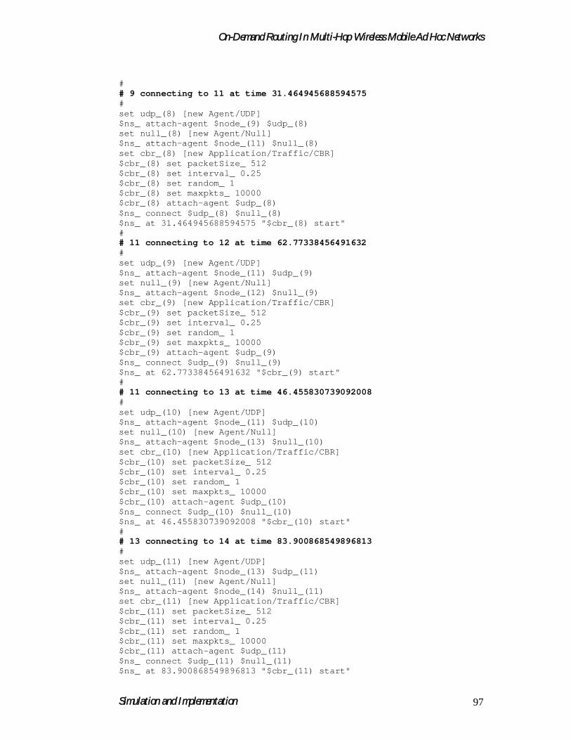
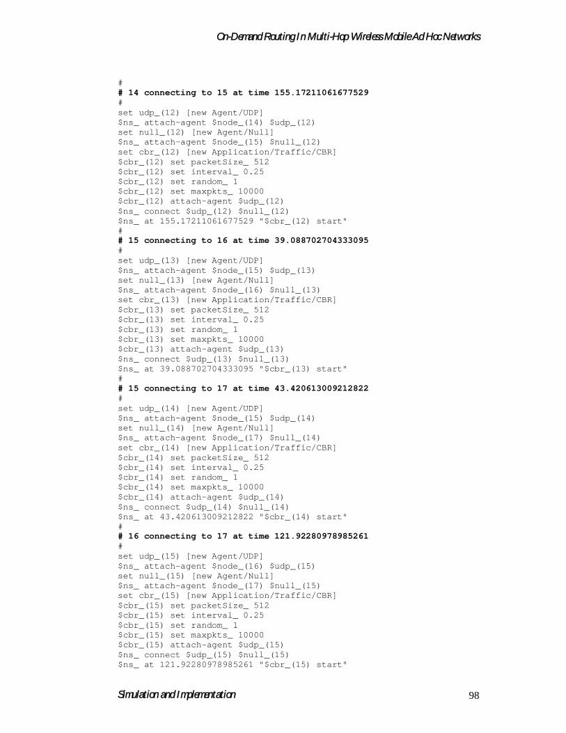
four files are generated for a given routing protocol. One of the traffic load generator
file (cbr-20-20-test) is enlisted as follows:
A Traffic Load Generation File (cbr-20-20-test)
## nodes: 50, max conn: 20, send rate: 0.25, seed: 1.0#

On-Demand Routing In Multi-Hop Wireless Mobile Ad Hoc Networks
Simulation and Implementation 95
## 1 connecting to 2 at time 2.5568388786897245#set udp_(0) [new Agent/UDP]$ns_ attach-agent $node_(1) $udp_(0)set null_(0) [new Agent/Null]$ns_ attach-agent $node_(2) $null_(0)set cbr_(0) [new Application/Traffic/CBR]$cbr_(0) set packetSize_ 512$cbr_(0) set interval_ 0.25$cbr_(0) set random_ 1$cbr_(0) set maxpkts_ 10000$cbr_(0) attach-agent $udp_(0)$ns_ connect $udp_(0) $null_(0)$ns_ at 2.5568388786897245 "$cbr_(0) start"## 4 connecting to 5 at time 56.333118917575632#set udp_(1) [new Agent/UDP]$ns_ attach-agent $node_(4) $udp_(1)set null_(1) [new Agent/Null]$ns_ attach-agent $node_(5) $null_(1)set cbr_(1) [new Application/Traffic/CBR]$cbr_(1) set packetSize_ 512$cbr_(1) set interval_ 0.25$cbr_(1) set random_ 1$cbr_(1) set maxpkts_ 10000$cbr_(1) attach-agent $udp_(1)$ns_ connect $udp_(1) $null_(1)$ns_ at 56.333118917575632 "$cbr_(1) start"## 4 connecting to 6 at time 146.96568928983328#set udp_(2) [new Agent/UDP]$ns_ attach-agent $node_(4) $udp_(2)set null_(2) [new Agent/Null]$ns_ attach-agent $node_(6) $null_(2)set cbr_(2) [new Application/Traffic/CBR]$cbr_(2) set packetSize_ 512$cbr_(2) set interval_ 0.25$cbr_(2) set random_ 1$cbr_(2) set maxpkts_ 10000$cbr_(2) attach-agent $udp_(2)$ns_ connect $udp_(2) $null_(2)$ns_ at 146.96568928983328 "$cbr_(2) start"## 6 connecting to 7 at time 55.634230382570173#set udp_(3) [new Agent/UDP]$ns_ attach-agent $node_(6) $udp_(3)set null_(3) [new Agent/Null]$ns_ attach-agent $node_(7) $null_(3)set cbr_(3) [new Application/Traffic/CBR]$cbr_(3) set packetSize_ 512$cbr_(3) set interval_ 0.25$cbr_(3) set random_ 1$cbr_(3) set maxpkts_ 10000$cbr_(3) attach-agent $udp_(3)$ns_ connect $udp_(3) $null_(3)$ns_ at 55.634230382570173 "$cbr_(3) start"

On-Demand Routing In Multi-Hop Wireless Mobile Ad Hoc Networks
Simulation and Implementation 96
## 7 connecting to 8 at time 29.546173154165118#set udp_(4) [new Agent/UDP]$ns_ attach-agent $node_(7) $udp_(4)set null_(4) [new Agent/Null]$ns_ attach-agent $node_(8) $null_(4)set cbr_(4) [new Application/Traffic/CBR]$cbr_(4) set packetSize_ 512$cbr_(4) set interval_ 0.25$cbr_(4) set random_ 1$cbr_(4) set maxpkts_ 10000$cbr_(4) attach-agent $udp_(4)$ns_ connect $udp_(4) $null_(4)$ns_ at 29.546173154165118 "$cbr_(4) start"## 7 connecting to 9 at time 7.7030203154790309#set udp_(5) [new Agent/UDP]$ns_ attach-agent $node_(7) $udp_(5)set null_(5) [new Agent/Null]$ns_ attach-agent $node_(9) $null_(5)set cbr_(5) [new Application/Traffic/CBR]$cbr_(5) set packetSize_ 512$cbr_(5) set interval_ 0.25$cbr_(5) set random_ 1$cbr_(5) set maxpkts_ 10000$cbr_(5) attach-agent $udp_(5)$ns_ connect $udp_(5) $null_(5)$ns_ at 7.7030203154790309 "$cbr_(5) start"## 8 connecting to 9 at time 20.48548468411224#set udp_(6) [new Agent/UDP]$ns_ attach-agent $node_(8) $udp_(6)set null_(6) [new Agent/Null]$ns_ attach-agent $node_(9) $null_(6)set cbr_(6) [new Application/Traffic/CBR]$cbr_(6) set packetSize_ 512$cbr_(6) set interval_ 0.25$cbr_(6) set random_ 1$cbr_(6) set maxpkts_ 10000$cbr_(6) attach-agent $udp_(6)$ns_ connect $udp_(6) $null_(6)$ns_ at 20.48548468411224 "$cbr_(6) start"## 9 connecting to 10 at time 76.258212521792487#set udp_(7) [new Agent/UDP]$ns_ attach-agent $node_(9) $udp_(7)set null_(7) [new Agent/Null]$ns_ attach-agent $node_(10) $null_(7)set cbr_(7) [new Application/Traffic/CBR]$cbr_(7) set packetSize_ 512$cbr_(7) set interval_ 0.25$cbr_(7) set random_ 1$cbr_(7) set maxpkts_ 10000$cbr_(7) attach-agent $udp_(7)$ns_ connect $udp_(7) $null_(7)$ns_ at 76.258212521792487 "$cbr_(7) start"
On-Demand Routing In Multi-Hop Wireless Mobile Ad Hoc Networks
Simulation and Implementation 97
## 9 connecting to 11 at time 31.464945688594575#set udp_(8) [new Agent/UDP]$ns_ attach-agent $node_(9) $udp_(8)set null_(8) [new Agent/Null]$ns_ attach-agent $node_(11) $null_(8)set cbr_(8) [new Application/Traffic/CBR]$cbr_(8) set packetSize_ 512$cbr_(8) set interval_ 0.25$cbr_(8) set random_ 1$cbr_(8) set maxpkts_ 10000$cbr_(8) attach-agent $udp_(8)$ns_ connect $udp_(8) $null_(8)$ns_ at 31.464945688594575 "$cbr_(8) start"## 11 connecting to 12 at time 62.77338456491632#set udp_(9) [new Agent/UDP]$ns_ attach-agent $node_(11) $udp_(9)set null_(9) [new Agent/Null]$ns_ attach-agent $node_(12) $null_(9)set cbr_(9) [new Application/Traffic/CBR]$cbr_(9) set packetSize_ 512$cbr_(9) set interval_ 0.25$cbr_(9) set random_ 1$cbr_(9) set maxpkts_ 10000$cbr_(9) attach-agent $udp_(9)$ns_ connect $udp_(9) $null_(9)$ns_ at 62.77338456491632 "$cbr_(9) start"## 11 connecting to 13 at time 46.455830739092008#set udp_(10) [new Agent/UDP]$ns_ attach-agent $node_(11) $udp_(10)set null_(10) [new Agent/Null]$ns_ attach-agent $node_(13) $null_(10)set cbr_(10) [new Application/Traffic/CBR]$cbr_(10) set packetSize_ 512$cbr_(10) set interval_ 0.25$cbr_(10) set random_ 1$cbr_(10) set maxpkts_ 10000$cbr_(10) attach-agent $udp_(10)$ns_ connect $udp_(10) $null_(10)$ns_ at 46.455830739092008 "$cbr_(10) start"## 13 connecting to 14 at time 83.900868549896813#set udp_(11) [new Agent/UDP]$ns_ attach-agent $node_(13) $udp_(11)set null_(11) [new Agent/Null]$ns_ attach-agent $node_(14) $null_(11)set cbr_(11) [new Application/Traffic/CBR]$cbr_(11) set packetSize_ 512$cbr_(11) set interval_ 0.25$cbr_(11) set random_ 1$cbr_(11) set maxpkts_ 10000$cbr_(11) attach-agent $udp_(11)$ns_ connect $udp_(11) $null_(11)$ns_ at 83.900868549896813 "$cbr_(11) start"
On-Demand Routing In Multi-Hop Wireless Mobile Ad Hoc Networks
Simulation and Implementation 98
## 14 connecting to 15 at time 155.17211061677529#set udp_(12) [new Agent/UDP]$ns_ attach-agent $node_(14) $udp_(12)set null_(12) [new Agent/Null]$ns_ attach-agent $node_(15) $null_(12)set cbr_(12) [new Application/Traffic/CBR]$cbr_(12) set packetSize_ 512$cbr_(12) set interval_ 0.25$cbr_(12) set random_ 1$cbr_(12) set maxpkts_ 10000$cbr_(12) attach-agent $udp_(12)$ns_ connect $udp_(12) $null_(12)$ns_ at 155.17211061677529 "$cbr_(12) start"## 15 connecting to 16 at time 39.088702704333095#set udp_(13) [new Agent/UDP]$ns_ attach-agent $node_(15) $udp_(13)set null_(13) [new Agent/Null]$ns_ attach-agent $node_(16) $null_(13)set cbr_(13) [new Application/Traffic/CBR]$cbr_(13) set packetSize_ 512$cbr_(13) set interval_ 0.25$cbr_(13) set random_ 1$cbr_(13) set maxpkts_ 10000$cbr_(13) attach-agent $udp_(13)$ns_ connect $udp_(13) $null_(13)$ns_ at 39.088702704333095 "$cbr_(13) start"## 15 connecting to 17 at time 43.420613009212822#set udp_(14) [new Agent/UDP]$ns_ attach-agent $node_(15) $udp_(14)set null_(14) [new Agent/Null]$ns_ attach-agent $node_(17) $null_(14)set cbr_(14) [new Application/Traffic/CBR]$cbr_(14) set packetSize_ 512$cbr_(14) set interval_ 0.25$cbr_(14) set random_ 1$cbr_(14) set maxpkts_ 10000$cbr_(14) attach-agent $udp_(14)$ns_ connect $udp_(14) $null_(14)$ns_ at 43.420613009212822 "$cbr_(14) start"## 16 connecting to 17 at time 121.92280978985261#set udp_(15) [new Agent/UDP]$ns_ attach-agent $node_(16) $udp_(15)set null_(15) [new Agent/Null]$ns_ attach-agent $node_(17) $null_(15)set cbr_(15) [new Application/Traffic/CBR]$cbr_(15) set packetSize_ 512$cbr_(15) set interval_ 0.25$cbr_(15) set random_ 1$cbr_(15) set maxpkts_ 10000$cbr_(15) attach-agent $udp_(15)$ns_ connect $udp_(15) $null_(15)$ns_ at 121.92280978985261 "$cbr_(15) start"
On-Demand Routing In Multi-Hop Wireless Mobile Ad Hoc Networks
Simulation and Implementation 99
## 16 connecting to 18 at time 137.20174070317378#set udp_(16) [new Agent/UDP]$ns_ attach-agent $node_(16) $udp_(16)set null_(16) [new Agent/Null]$ns_ attach-agent $node_(18) $null_(16)set cbr_(16) [new Application/Traffic/CBR]$cbr_(16) set packetSize_ 512$cbr_(16) set interval_ 0.25$cbr_(16) set random_ 1$cbr_(16) set maxpkts_ 10000$cbr_(16) attach-agent $udp_(16)$ns_ connect $udp_(16) $null_(16)$ns_ at 137.20174070317378 "$cbr_(16) start"## 17 connecting to 18 at time 72.99343390995331#set udp_(17) [new Agent/UDP]$ns_ attach-agent $node_(17) $udp_(17)set null_(17) [new Agent/Null]$ns_ attach-agent $node_(18) $null_(17)set cbr_(17) [new Application/Traffic/CBR]$cbr_(17) set packetSize_ 512$cbr_(17) set interval_ 0.25$cbr_(17) set random_ 1$cbr_(17) set maxpkts_ 10000$cbr_(17) attach-agent $udp_(17)$ns_ connect $udp_(17) $null_(17)$ns_ at 72.99343390995331 "$cbr_(17) start"## 17 connecting to 19 at time 19.655724884781858#set udp_(18) [new Agent/UDP]$ns_ attach-agent $node_(17) $udp_(18)set null_(18) [new Agent/Null]$ns_ attach-agent $node_(19) $null_(18)set cbr_(18) [new Application/Traffic/CBR]$cbr_(18) set packetSize_ 512$cbr_(18) set interval_ 0.25$cbr_(18) set random_ 1$cbr_(18) set maxpkts_ 10000$cbr_(18) attach-agent $udp_(18)$ns_ connect $udp_(18) $null_(18)$ns_ at 19.655724884781858 "$cbr_(18) start"##Total sources/connections: 12/19#
5.2.2 Mobility Generation Models
The movement scenario files used for each simulation are characterized by a
pause time. To study the effect of mobility, the simulation is carried out with
movement patterns generated for different pause times. Pause time of 0 seconds

On-Demand Routing In Multi-Hop Wireless Mobile Ad Hoc Networks
Simulation and Implementation 100
--(5.11)
corresponding to continuous motion, and a pause time of 100 corresponds to almost
no motion. A set of movement scenario files corresponds to different mobility is
created by varying pause time. The ‘setdest’ program of NS-2 simulators is used to
generate node-movement files using the ‘Random Waypoint Algorithm’.
To study the effect of mobility, pause time can be varied from 0 seconds (high
mobility) to 100 seconds (low mobility). However in simulation study sample pause
time of 0, 10, 20, 30, 40 and 100 sec were considered.
The command (5.10) used to generate random movements of nodes as
follows-
./setdest [-v version ] [-n num_of_nodes] [-p pausetime] [-M maxspeed] [-t
simtime] [-x maxx] [-y maxy] > [outdir/movement-file] > movement-file.---- (5.10)
For a pause time of 0, 10, 20, 30, 40 and 100 the corresponding mobility files
are generated in the directory “~ns/indep-utils/cmu-scen-gen/setdest/” as follows-
./setdest - v 1 -n 50 –p 0 –M 20 –t 200 –x 500 –y 500>scen-0-20-test
./setdest - v 1 -n 50 –p10 –M 20 –t 200 –x 500 –y 500>scen-10-20-test
./setdest - v 1 -n 50 –p20 –M 20 –t 200 –x 500 –y 500>scen-20-20-test
./setdest - v 1 -n 50 –p30 –M 20 –t 200 –x 500 –y 500>scen-30-20-test
./setdest - v 1 -n 50 –p40 –M 20 –t 200 –x 500 –y 500>scen-40-20-test
./setdest - v 1 -n 50 –p100 –M 20 –t 200 –x 500 –y 500>scen-100-20-test
The set of files (5.11) with varying pause time corresponds to number of nodes
50. When the pause time of nodes is varied, for each pause time six files are to be
recreated. For pause time 0, 10, 20, 30, 40 and 100 sec six files are created for one
routing protocol. One of the mobility file (scen-0-20-test) is as follows-
## nodes: 50, pause: 0.00, max speed: 20.00, max x: 500.00, max y: 500.00#$node_(0) set X_ 291.980439385383$node_(0) set Y_ 27.275766519215$node_(0) set Z_ 0.000000000000$node_(1) set X_ 214.304622862339$node_(1) set Y_ 425.622983726110$node_(1) set Z_ 0.000000000000

On-Demand Routing In Multi-Hop Wireless Mobile Ad Hoc Networks
Simulation and Implementation 101
$node_(2) set X_ 396.759502246505$node_(2) set Y_ 282.896475829758$node_(2) set Z_ 0.000000000000$node_(3) set X_ 436.638885834461$node_(3) set Y_ 484.596795122170$node_(3) set Z_ 0.000000000000$node_(4) set X_ 410.272734201683$node_(4) set Y_ 353.017376369707$node_(4) set Z_ 0.000000000000$node_(5) set X_ 57.360732562615$node_(5) set Y_ 478.120438044204$node_(5) set Z_ 0.000000000000$node_(6) set X_ 497.664558355284$node_(6) set Y_ 54.465532728664$node_(6) set Z_ 0.000000000000$node_(7) set X_ 256.535756601821$node_(7) set Y_ 336.292332142779$node_(7) set Z_ 0.000000000000$node_(8) set X_ 82.362449758544$node_(8) set Y_ 134.067252601029$node_(8) set Z_ 0.000000000000$node_(9) set X_ 299.236249816869$node_(9) set Y_ 458.103517951800$node_(9) set Z_ 0.000000000000$node_(10) set X_ 79.076194075832$node_(10) set Y_ 22.489663604146$node_(10) set Z_ 0.000000000000$node_(11) set X_ 395.819531132109$node_(11) set Y_ 310.158664596500$node_(11) set Z_ 0.000000000000$node_(12) set X_ 191.100156923950$node_(12) set Y_ 280.059097975561$node_(12) set Z_ 0.000000000000$node_(13) set X_ 365.921242421404$node_(13) set Y_ 160.228908836752$node_(13) set Z_ 0.000000000000$node_(14) set X_ 482.883048928267$node_(14) set Y_ 369.575374497026$node_(14) set Z_ 0.000000000000$node_(15) set X_ 477.334028874868$node_(15) set Y_ 388.680770258792$node_(15) set Z_ 0.000000000000$node_(16) set X_ 120.762825854744$node_(16) set Y_ 465.118867402134$node_(16) set Z_ 0.000000000000$node_(17) set X_ 402.373515347413$node_(17) set Y_ 123.823614384819$node_(17) set Z_ 0.000000000000$node_(18) set X_ 371.630110731130$node_(18) set Y_ 153.184877094453$node_(18) set Z_ 0.000000000000$node_(19) set X_ 170.347823279991$node_(19) set Y_ 303.262520366955$node_(19) set Z_ 0.000000000000$ns_ at 0.000000000000 "$node_(0) setdest 332.336751191421 305.271940421444 19.185880588056"$ns_ at 0.000000000000 "$node_(1) setdest 240.454421498468 462.942545952287 0.699285302649"$ns_ at 0.000000000000 "$node_(2) setdest 159.154424002422 332.341179164817 16.222733863240"

On-Demand Routing In Multi-Hop Wireless Mobile Ad Hoc Networks
Simulation and Implementation 102
$ns_ at 0.000000000000 "$node_(3) setdest 88.030285507045 304.249250861780 0.585914371039"$ns_ at 0.000000000000 "$node_(4) setdest 478.495400870928 373.598971103455 7.603100207971"$ns_ at 0.000000000000 "$node_(5) setdest 412.515233108580 146.883227758042 12.049079725102"$ns_ at 0.000000000000 "$node_(6) setdest 251.494998766798 320.144019809076 10.410035388844"$ns_ at 0.000000000000 "$node_(7) setdest 183.905387938097 31.686551424396 18.803266899446"$ns_ at 0.000000000000 "$node_(8) setdest 102.949996691570 101.974828334238 6.261038277833"$ns_ at 0.000000000000 "$node_(9) setdest 444.097444851014 455.283749429281 5.690157959134"$ns_ at 0.000000000000 "$node_(10) setdest 361.039244126566 293.288092828338 4.210243736331"$ns_ at 0.000000000000 "$node_(11) setdest 340.711947034133 239.546081243452 4.475012619701"$ns_ at 0.000000000000 "$node_(12) setdest 227.921613237750 105.066155282259 15.670119267745"$ns_ at 0.000000000000 "$node_(13) setdest 128.107961184917 415.416889802253 14.198642590390"$ns_ at 0.000000000000 "$node_(14) setdest 437.697480325838 414.591332253767 6.724746585532"$ns_ at 0.000000000000 "$node_(15) setdest 181.801537707150 10.018302030816 9.774664322177"$ns_ at 0.000000000000 "$node_(16) setdest 62.868571858076 67.493085176349 4.201355980216"$ns_ at 0.000000000000 "$node_(17) setdest 177.778019797483 318.481720691593 10.130137849382"$ns_ at 0.000000000000 "$node_(18) setdest 292.223195261887 445.769473379490 0.234632587247"$ns_ at 0.000000000000 "$node_(19) setdest 26.129414079459 492.333725771265 17.071013886195"$god_ set-dist 0 1 3$god_ set-dist 0 2 2$god_ set-dist 0 3 3$god_ set-dist 0 4 2$god_ set-dist 0 5 3$god_ set-dist 0 6 1$god_ set-dist 0 7 2$god_ set-dist 0 8 1$god_ set-dist 0 9 3$god_ set-dist 0 10 1$god_ set-dist 0 11 2$god_ set-dist 0 12 2$god_ set-dist 0 13 1$god_ set-dist 0 14 2$god_ set-dist 0 15 3$god_ set-dist 0 16 3$god_ set-dist 0 17 1$god_ set-dist 0 18 1$god_ set-dist 0 19 2$god_ set-dist 1 2 1$god_ set-dist 1 3 1$god_ set-dist 1 4 1$god_ set-dist 1 5 1$god_ set-dist 1 6 2$god_ set-dist 1 7 1$god_ set-dist 1 8 2

On-Demand Routing In Multi-Hop Wireless Mobile Ad Hoc Networks
Simulation and Implementation 103
$god_ set-dist 1 9 1$god_ set-dist 1 10 3$god_ set-dist 1 11 1$god_ set-dist 1 12 1$god_ set-dist 1 13 2$god_ set-dist 1 14 2$god_ set-dist 1 15 2$god_ set-dist 1 16 1$god_ set-dist 1 17 2$god_ set-dist 1 18 2$god_ set-dist 1 19 1$god_ set-dist 2 3 1$god_ set-dist 2 4 1$god_ set-dist 2 5 2$god_ set-dist 2 6 1$god_ set-dist 2 7 1$god_ set-dist 2 8 2$god_ set-dist 2 9 1$god_ set-dist 2 10 3$god_ set-dist 2 11 1$god_ set-dist 2 12 1$god_ set-dist 2 13 1$god_ set-dist 2 14 1$god_ set-dist 2 15 1$god_ set-dist 2 16 2$god_ set-dist 2 17 1$god_ set-dist 2 18 1$god_ set-dist 2 19 1$god_ set-dist 3 4 1$god_ set-dist 3 5 2$god_ set-dist 3 6 2$god_ set-dist 3 7 1$god_ set-dist 3 8 3$god_ set-dist 3 9 1$god_ set-dist 3 10 4$god_ set-dist 3 11 1$god_ set-dist 3 12 2$god_ set-dist 3 13 2$god_ set-dist 3 14 1$god_ set-dist 3 15 1$god_ set-dist 3 16 2$god_ set-dist 3 17 2$god_ set-dist 3 18 2$god_ set-dist 3 19 2$god_ set-dist 4 5 2$god_ set-dist 4 6 2$god_ set-dist 4 7 1$god_ set-dist 4 8 2$god_ set-dist 4 9 1$god_ set-dist 4 10 3$god_ set-dist 4 11 1$god_ set-dist 4 12 1$god_ set-dist 4 13 1$god_ set-dist 4 14 1$god_ set-dist 4 15 1$god_ set-dist 4 16 2$god_ set-dist 4 17 1$god_ set-dist 4 18 1$god_ set-dist 4 19 1$god_ set-dist 5 6 3

On-Demand Routing In Multi-Hop Wireless Mobile Ad Hoc Networks
Simulation and Implementation 104
$god_ set-dist 5 7 1$god_ set-dist 5 8 2$god_ set-dist 5 9 1$god_ set-dist 5 10 3$god_ set-dist 5 11 2$god_ set-dist 5 12 1$god_ set-dist 5 13 2$god_ set-dist 5 14 2$god_ set-dist 5 15 2$god_ set-dist 5 16 1$god_ set-dist 5 17 3$god_ set-dist 5 18 2$god_ set-dist 5 19 1$god_ set-dist 6 7 2$god_ set-dist 6 8 2$god_ set-dist 6 9 2$god_ set-dist 6 10 2$god_ set-dist 6 11 2$god_ set-dist 6 12 2$god_ set-dist 6 13 1$god_ set-dist 6 14 2$god_ set-dist 6 15 2$god_ set-dist 6 16 3$god_ set-dist 6 17 1$god_ set-dist 6 18 1$god_ set-dist 6 19 2$god_ set-dist 7 8 2$god_ set-dist 7 9 1$god_ set-dist 7 10 3$god_ set-dist 7 11 1$god_ set-dist 7 12 1$god_ set-dist 7 13 1$god_ set-dist 7 14 1$god_ set-dist 7 15 1$god_ set-dist 7 16 1$god_ set-dist 7 17 2$god_ set-dist 7 18 1$god_ set-dist 7 19 1$god_ set-dist 8 9 2$god_ set-dist 8 10 1$god_ set-dist 8 11 2$god_ set-dist 8 12 1$god_ set-dist 8 13 2$god_ set-dist 8 14 3$god_ set-dist 8 15 3$god_ set-dist 8 16 2$god_ set-dist 8 17 2$god_ set-dist 8 18 2$god_ set-dist 8 19 1$god_ set-dist 9 10 3$god_ set-dist 9 11 1$god_ set-dist 9 12 1$god_ set-dist 9 13 2$god_ set-dist 9 14 1$god_ set-dist 9 15 1$god_ set-dist 9 16 1$god_ set-dist 9 17 2$god_ set-dist 9 18 2$god_ set-dist 9 19 1$god_ set-dist 10 11 3
On-Demand Routing In Multi-Hop Wireless Mobile Ad Hoc Networks
Simulation and Implementation 105
$god_ set-dist 10 12 2$god_ set-dist 10 13 2$god_ set-dist 10 14 3$god_ set-dist 10 15 4$god_ set-dist 10 16 3$god_ set-dist 10 17 2$god_ set-dist 10 18 2$god_ set-dist 10 19 2$god_ set-dist 11 12 1$god_ set-dist 11 13 1$god_ set-dist 11 14 1$god_ set-dist 11 15 1$god_ set-dist 11 16 2$god_ set-dist 11 17 1$god_ set-dist 11 18 1$god_ set-dist 11 19 1$god_ set-dist 12 13 1$god_ set-dist 12 14 2$god_ set-dist 12 15 2$god_ set-dist 12 16 1$god_ set-dist 12 17 2$god_ set-dist 12 18 1$god_ set-dist 12 19 1$god_ set-dist 13 14 1$god_ set-dist 13 15 2$god_ set-dist 13 16 2$god_ set-dist 13 17 1$god_ set-dist 13 18 1$god_ set-dist 13 19 1$god_ set-dist 14 15 1$god_ set-dist 14 16 2$god_ set-dist 14 17 2$god_ set-dist 14 18 1$god_ set-dist 14 19 2$god_ set-dist 15 16 2$god_ set-dist 15 17 2$god_ set-dist 15 18 2$god_ set-dist 15 19 2$god_ set-dist 16 17 3$god_ set-dist 16 18 2$god_ set-dist 16 19 1$god_ set-dist 17 18 1$god_ set-dist 17 19 2$god_ set-dist 18 19 2$ns_ at 0.286039706347 "$god_ set-dist 0 15 2"$ns_ at 0.286039706347 "$god_ set-dist 10 15 3"$ns_ at 0.286039706347 "$god_ set-dist 13 15 1"$ns_ at 0.329220721329 "$god_ set-dist 4 19 2"$ns_ at 0.345113893503 "$god_ set-dist 5 17 2"$ns_ at 0.345113893503 "$god_ set-dist 7 17 1"$ns_ at 0.345113893503 "$god_ set-dist 16 17 2"$ns_ at 0.589273388271 "$god_ set-dist 12 17 1"$ns_ at 0.696264154542 "$god_ set-dist 0 1 2"$ns_ at 0.696264154542 "$god_ set-dist 0 5 2"$ns_ at 0.696264154542 "$god_ set-dist 0 9 2"$ns_ at 0.696264154542 "$god_ set-dist 0 12 1"$ns_ at 0.696264154542 "$god_ set-dist 0 16 2"$ns_ at 0.841198488493 "$god_ set-dist 15 18 1"$ns_ at 1.133505248928 "$god_ set-dist 3 8 2"$ns_ at 1.133505248928 "$god_ set-dist 3 10 3"
On-Demand Routing In Multi-Hop Wireless Mobile Ad Hoc Networks
Simulation and Implementation 106
$ns_ at 1.133505248928 "$god_ set-dist 7 8 1"$ns_ at 1.133505248928 "$god_ set-dist 7 10 2"$ns_ at 1.133505248928 "$god_ set-dist 8 14 2"$ns_ at 1.133505248928 "$god_ set-dist 8 15 2"$ns_ at 1.134217939316 "$god_ set-dist 3 7 2"$ns_ at 1.134217939316 "$god_ set-dist 3 8 3"$ns_ at 1.134217939316 "$god_ set-dist 3 10 4"$ns_ at 1.235051939714 "$god_ set-dist 0 2 1"$ns_ at 1.235051939714 "$god_ set-dist 0 3 2"$ns_ at 1.235051939714 "$god_ set-dist 2 10 2"$ns_ at 1.235051939714 "$god_ set-dist 3 10 3"$ns_ at 1.705783448641 "$god_ set-dist 0 7 1"$ns_ at 1.852523240518 "$god_ set-dist 4 12 2"$ns_ at 1.876757993435 "$god_ set-dist 1 10 2"$ns_ at 1.876757993435 "$god_ set-dist 5 10 2"$ns_ at 1.876757993435 "$god_ set-dist 9 10 2"$ns_ at 1.876757993435 "$god_ set-dist 10 11 2"$ns_ at 1.876757993435 "$god_ set-dist 10 12 1"$ns_ at 1.876757993435 "$god_ set-dist 10 16 2"$ns_ at 1.908396611796 "$god_ set-dist 15 17 1"$ns_ at 2.107621039562 "$god_ set-dist 6 11 1"$ns_ at 2.231710964265 "$god_ set-dist 0 11 1"$ns_ at 2.631746715853 "$god_ set-dist 2 6 2"$ns_ at 2.787112517637 "$god_ set-dist 11 19 2"$ns_ at 2.878368916953 "$god_ set-dist 9 10 3"$ns_ at 2.878368916953 "$god_ set-dist 9 12 2"$ns_ at 3.139612404635 "$god_ set-dist 6 19 3"$ns_ at 3.139612404635 "$god_ set-dist 13 19 2"$ns_ at 3.158716057276 "$god_ set-dist 14 18 2"$ns_ at 3.283401798393 "$god_ set-dist 7 14 2"$ns_ at 3.283401798393 "$god_ set-dist 8 14 3"$ns_ at 3.361630896329 "$god_ set-dist 1 15 1"$ns_ at 3.365050551202 "$god_ set-dist 5 10 3"$ns_ at 3.365050551202 "$god_ set-dist 5 12 2"$ns_ at 3.673507355736 "$god_ set-dist 8 13 1"$ns_ at 3.673507355736 "$god_ set-dist 8 14 2"$ns_ at 4.153770753946 "$god_ set-dist 1 13 1"$ns_ at 4.177530228262 "$god_ set-dist 1 14 1"$ns_ at 4.189551685039 "$god_ set-dist 8 19 2"$ns_ at 4.404947834646 "$god_ set-dist 10 16 3"$ns_ at 4.404947834646 "$god_ set-dist 12 16 2"$ns_ at 4.562571285149 "$god_ set-dist 9 13 1"$ns_ at 4.800853935213 "$god_ set-dist 2 16 1"$ns_ at 5.036758029293 "$god_ set-dist 4 10 2"$ns_ at 5.036758029293 "$god_ set-dist 5 10 2"$ns_ at 5.036758029293 "$god_ set-dist 7 10 1"$ns_ at 5.036758029293 "$god_ set-dist 9 10 2"$ns_ at 5.036758029293 "$god_ set-dist 10 15 2"$ns_ at 5.036758029293 "$god_ set-dist 10 16 2"$ns_ at 5.223943248836 "$god_ set-dist 2 5 1"$ns_ at 5.338228063760 "$god_ set-dist 4 7 2"$ns_ at 5.338228063760 "$god_ set-dist 4 10 3"$ns_ at 5.516665167517 "$god_ set-dist 6 15 1"$ns_ at 5.671408493321 "$god_ set-dist 0 15 1"$ns_ at 5.863590943515 "$god_ set-dist 7 9 2"$ns_ at 5.863590943515 "$god_ set-dist 9 10 3"$ns_ at 6.089780082675 "$node_(8) setdest 474.829529473684 492.384947816857 14.625592665310"$ns_ at 6.540271423650 "$god_ set-dist 5 6 2"$ns_ at 6.540271423650 "$god_ set-dist 6 7 1"

On-Demand Routing In Multi-Hop Wireless Mobile Ad Hoc Networks
Simulation and Implementation 107
$ns_ at 6.540271423650 "$god_ set-dist 6 16 2"$ns_ at 6.540271423650 "$god_ set-dist 6 19 2"$ns_ at 6.562677000109 "$god_ set-dist 1 12 2"$ns_ at 6.586893332104 "$god_ set-dist 6 12 1"$ns_ at 6.659713883894 "$god_ set-dist 8 17 1"$ns_ at 6.732451513695 "$god_ set-dist 1 4 2"$ns_ at 6.755577868899 "$god_ set-dist 6 16 3"$ns_ at 6.755577868899 "$god_ set-dist 7 16 2"$ns_ at 6.755577868899 "$god_ set-dist 8 16 3"$ns_ at 6.755577868899 "$god_ set-dist 10 16 3"$ns_ at 6.888778072638 "$god_ set-dist 12 19 2"$ns_ at 7.136290191355 "$god_ set-dist 9 19 2"$ns_ at 7.359085883518 "$god_ set-dist 5 13 1"$ns_ at 7.468066777935 "$god_ set-dist 2 8 1"$ns_ at 7.468066777935 "$god_ set-dist 3 8 2"$ns_ at 7.468066777935 "$god_ set-dist 8 16 2"$ns_ at 7.611870527566 "$god_ set-dist 0 4 1"$ns_ at 7.611870527566 "$god_ set-dist 4 10 2"$ns_ at 7.694028271413 "$god_ set-dist 6 19 3"$ns_ at 7.694028271413 "$god_ set-dist 7 19 2"$ns_ at 7.694028271413 "$god_ set-dist 10 19 3"$ns_ at 8.081019460631 "$god_ set-dist 0 10 2"$ns_ at 8.081019460631 "$god_ set-dist 4 10 3"$ns_ at 8.093843234774 "$god_ set-dist 8 18 1"$ns_ at 8.277899925008 "$god_ set-dist 7 15 2"$ns_ at 8.277899925008 "$god_ set-dist 10 15 3"$ns_ at 8.331144865570 "$god_ set-dist 6 16 2"$ns_ at 8.331144865570 "$god_ set-dist 13 16 1"$ns_ at 8.517313702683 "$god_ set-dist 1 7 2"$ns_ at 8.517313702683 "$god_ set-dist 1 10 3"$ns_ at 8.817008211337 "$god_ set-dist 0 14 1"$ns_ at 9.172519213700 "$god_ set-dist 0 1 1"$ns_ at 9.372443344396 "$node_(4) setdest 446.232664705346 329.048175351233 10.509290608096"$ns_ at 9.462899737800 "$god_ set-dist 2 3 2"$ns_ at 9.462899737800 "$god_ set-dist 3 8 3"$ns_ at 9.484702941421 "$node_(14) setdest 200.392468176231 172.082789426954 13.705691278629"$ns_ at 9.500821821766 "$god_ set-dist 4 6 1"$ns_ at 9.600605755257 "$god_ set-dist 0 9 1"$ns_ at 9.619414283236 "$god_ set-dist 14 17 1"$ns_ at 9.709271912617 "$god_ set-dist 5 7 2"$ns_ at 9.709271912617 "$god_ set-dist 5 10 3"$ns_ at 9.980348502213 "$god_ set-dist 0 5 1"$ns_ at 10.136726394527 "$god_ set-dist 5 8 1"$ns_ at 10.136726394527 "$god_ set-dist 5 10 2"$ns_ at 10.288313827509 "$god_ set-dist 5 11 1"$ns_ at 10.626637509103 "$god_ set-dist 3 8 2"$ns_ at 10.626637509103 "$god_ set-dist 8 11 1"$ns_ at 10.921751060184 "$god_ set-dist 9 16 2"$ns_ at 10.965695065857 "$god_ set-dist 14 18 1"$ns_ at 11.011630825802 "$god_ set-dist 4 10 2"$ns_ at 11.011630825802 "$god_ set-dist 10 14 2"$ns_ at 11.011630825802 "$god_ set-dist 10 15 2"$ns_ at 11.011630825802 "$god_ set-dist 10 17 1"$ns_ at 11.036949210122 "$god_ set-dist 2 4 2"$ns_ at 11.036949210122 "$god_ set-dist 4 19 3"$ns_ at 11.073013364176 "$god_ set-dist 5 17 1"$ns_ at 11.411841244003 "$node_(12) setdest 157.367520786925 495.410109298607 17.608776782319"
On-Demand Routing In Multi-Hop Wireless Mobile Ad Hoc Networks
Simulation and Implementation 108
$ns_ at 11.608076923868 "$god_ set-dist 1 10 2"$ns_ at 11.608076923868 "$god_ set-dist 1 17 1"$ns_ at 11.647756939247 "$god_ set-dist 6 14 1"$ns_ at 11.977083307462 "$god_ set-dist 0 3 1"$ns_ at 12.038241530329 "$god_ set-dist 5 14 1"$ns_ at 12.051624738218 "$god_ set-dist 6 8 1"$ns_ at 12.233014232540 "$god_ set-dist 12 15 1"$ns_ at 12.423150747293 "$god_ set-dist 5 15 1"$ns_ at 12.442170636276 "$god_ set-dist 8 16 1"$ns_ at 12.442170636276 "$god_ set-dist 10 16 2"$ns_ at 12.785217101078 "$god_ set-dist 5 12 1"$ns_ at 13.145245529834 "$god_ set-dist 8 15 1"$ns_ at 13.160922165933 "$god_ set-dist 2 18 2"$ns_ at 13.160922165933 "$god_ set-dist 18 19 3"$ns_ at 13.532108320912 "$god_ set-dist 0 16 1"$ns_ at 13.929802879368 "$node_(19) setdest 167.461129564772 373.627941523355 19.863319110957"$ns_ at 13.940057021243 "$god_ set-dist 0 7 2"$ns_ at 14.007428286354 "$god_ set-dist 2 7 2"$ns_ at 14.007428286354 "$god_ set-dist 7 19 3"$ns_ at 14.058928547900 "$god_ set-dist 1 8 1"$ns_ at 14.261281565734 "$god_ set-dist 1 4 1"$ns_ at 14.261281565734 "$god_ set-dist 4 19 2"$ns_ at 14.543356384834 "$god_ set-dist 2 9 2"$ns_ at 14.606476679932 "$node_(4) setdest 387.233625409332 369.228457054011 15.681001609575"$ns_ at 14.622239133471 "$god_ set-dist 3 7 3"$ns_ at 14.622239133471 "$god_ set-dist 7 11 2"$ns_ at 14.641503416406 "$node_(0) setdest 8.956750240876 326.871654714761 14.134315224350"$ns_ at 14.745068474552 "$god_ set-dist 6 19 2"$ns_ at 14.745068474552 "$god_ set-dist 7 19 2"$ns_ at 14.745068474552 "$god_ set-dist 13 19 1"$ns_ at 14.745068474552 "$god_ set-dist 18 19 2"$ns_ at 14.790838778469 "$god_ set-dist 7 9 3"$ns_ at 14.790838778469 "$god_ set-dist 7 13 2"$ns_ at 14.790838778469 "$god_ set-dist 7 19 3"$ns_ at 14.960190134186 "$node_(2) setdest 139.052306400351 476.823072805814 7.145424901100"$ns_ at 15.094126606895 "$god_ set-dist 8 14 1"$ns_ at 15.097366159028 "$god_ set-dist 16 17 1"$ns_ at 15.111804777007 "$god_ set-dist 4 5 1"$ns_ at 15.252502254853 "$god_ set-dist 12 14 1"$ns_ at 15.381201657674 "$god_ set-dist 12 16 1"$ns_ at 16.019166202736 "$god_ set-dist 1 12 1"$ns_ at 16.091921361288 "$god_ set-dist 5 6 1"$ns_ at 16.520659966979 "$god_ set-dist 5 18 1"$ns_ at 16.598640007869 "$god_ set-dist 4 8 1"$ns_ at 16.653760178599 "$node_(7) setdest 91.814713458871 169.507971791937 17.705202047406"$ns_ at 17.218998140341 "$god_ set-dist 4 12 1"$ns_ at 17.221787682575 "$god_ set-dist 13 18 2"$ns_ at 17.594647317126 "$god_ set-dist 0 19 1"$ns_ at 17.676911962633 "$god_ set-dist 2 4 1"$ns_ at 18.034599582785 "$god_ set-dist 7 19 2"$ns_ at 18.034599582785 "$god_ set-dist 10 19 2"$ns_ at 18.034599582785 "$god_ set-dist 12 19 1"$ns_ at 18.069456182920 "$god_ set-dist 8 19 1"$ns_ at 18.177464344223 "$god_ set-dist 10 18 1"$ns_ at 18.434564907497 "$god_ set-dist 14 16 1"

On-Demand Routing In Multi-Hop Wireless Mobile Ad Hoc Networks
Simulation and Implementation 109
$ns_ at 18.491529427212 "$god_ set-dist 17 19 1"$ns_ at 18.847355012638 "$god_ set-dist 3 11 2"$ns_ at 19.158587815246 "$node_(4) setdest 456.475038418269 283.560004895665 19.018129817157"$ns_ at 19.408245626478 "$god_ set-dist 9 13 2"$ns_ at 19.509739297332 "$god_ set-dist 3 15 2"$ns_ at 19.595449180405 "$god_ set-dist 7 9 2"$ns_ at 19.595449180405 "$god_ set-dist 7 11 1"$ns_ at 19.645885489054 "$god_ set-dist 14 19 1"$ns_ at 19.809918337174 "$god_ set-dist 5 7 1"## Destination Unreachables: 0## Route Changes: 186## Link Changes: 113## Node | Route Changes | Link Changes# 0 | 21 | 15# 1 | 15 | 11# 2 | 12 | 11# 3 | 15 | 5# 4 | 19 | 12# 5 | 23 | 15# 6 | 17 | 9# 7 | 28 | 20# 8 | 26 | 15# 9 | 15 | 8# 10 | 40 | 5# 11 | 9 | 8# 12 | 17 | 17# 13 | 11 | 11# 14 | 16 | 12# 15 | 17 | 11# 16 | 22 | 10# 17 | 12 | 10# 18 | 10 | 8# 19 | 27 | 13#
5.2.3 Performance Evaluation Metrics
To evaluate the performance of routing protocols various quantitative metrics
are practiced [118]. In our research study six different quantitative metrics have been
used to compare the performance of routing protocols against mobility of the nodes
and traffic load conditions.
The six important performance metrics are considered for evaluation of these
routing protocols are as follows-

On-Demand Routing In Multi-Hop Wireless Mobile Ad Hoc Networks
Simulation and Implementation 110
1. Throughput - Throughput is the measure of how fast we can actually send
packets through network. The number of packets delivered to the receiver
provides the throughput of the network. The throughput is defined as the total
amount of data a receiver actually receives from the sender divided by the
time it takes for receiver to get the last packet [119].
2. Packets Dropped - Some of the packets generated by the source will get
dropped in the network due to high mobility of the nodes, congestion of the
network etc.
3. Packet Delivery Ratio - The ratio of the data packets delivered to the
destinations to those generated by the CBR sources. It is the fraction of
packets sent by the application that are received by the receivers [66].
4. Normalized Routing Overhead - The number of routing packets transmitted
per data packet delivered at the destination. Each hop-wise transmission of a
routing packet is counted as one transmission. The routing overhead describes
how many routing packets for route discovery and route maintenance need to
be sent in order to propagate the data packets [67].
5. End-to-End Delay – End-to-End delay indicates how long it took for a packet
to travel from the source to the application layer of the destination. [65]. i.e. the
total time taken by each packet to reach the destination. Average End-to-End
delay of data packets includes all possible delays caused by buffering during
route discovery, queuing delay at the interface, retransmission delays at the
MAC, propagation and transfer times.
6. Optimal Path Length - It is the ratio of total forwarding times (depends on
number of hops) to the total number of received packets. Optimal path length
increases as the number of hops on optimal path increases.
On-Demand Routing In Multi-Hop Wireless Mobile Ad Hoc Networks
Simulation and Implementation 111
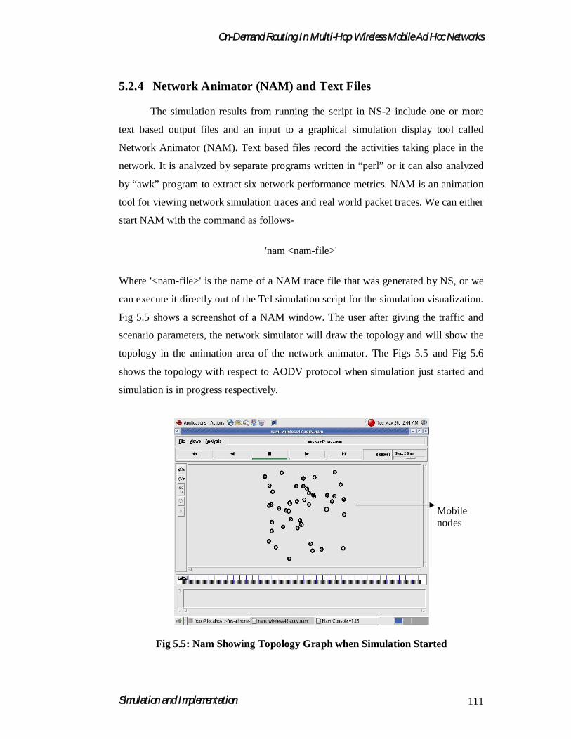
5.2.4 Network Animator (NAM) and Text Files
The simulation results from running the script in NS-2 include one or more
text based output files and an input to a graphical simulation display tool called
Network Animator (NAM). Text based files record the activities taking place in the
network. It is analyzed by separate programs written in “perl” or it can also analyzed
by “awk” program to extract six network performance metrics. NAM is an animation
tool for viewing network simulation traces and real world packet traces. We can either
start NAM with the command as follows-
'nam <nam-file>'
Where '<nam-file>' is the name of a NAM trace file that was generated by NS, or we
can execute it directly out of the Tcl simulation script for the simulation visualization.
Fig 5.5 shows a screenshot of a NAM window. The user after giving the traffic and
scenario parameters, the network simulator will draw the topology and will show the
topology in the animation area of the network animator. The Figs 5.5 and Fig 5.6
shows the topology with respect to AODV protocol when simulation just started and
simulation is in progress respectively.
Mobile nodes
Fig 5.5: Nam Showing Topology Graph when Simulation Started

On-Demand Routing In Multi-Hop Wireless Mobile Ad Hoc Networks
Simulation and Implementation 112
Fig 5.6: NAM Showing Topology Graph when Simulation in Progress
The Fig 5.7 shows the part of output snapshot that describes the trace file for
all the 50 nodes with maximum connections of 20. The trace file contains the sent
packets and also the received packets with the simulation times along with
instantaneous inter-node connections.
Fig 5.7: Output Snapshot that describes the Trace File

On-Demand Routing In Multi-Hop Wireless Mobile Ad Hoc Networks
Simulation and Implementation 113
5.3 COMPARISON OF SIMULATION RESULTS OF DSDV, DSR AND AODV (Unipath routing protocols)
5.3.1 Simulation Results: EFFECT OF MOBILITY
To analyze the effect of mobility, pause time was varied from 0 seconds (high
mobility) to 100 seconds (low mobility). The number of nodes is taken as 50 and the
maximum number of connection as 20. Graphs shown in Fig 5.8 (a-f) show the effect
of Mobility for DSDV, DSR and AODV protocols with respect to various
performance metrics.
5.3.1 (a) Throughput
Table 5.9(a): Pause Time Vs Throughput (bits/sec)
Pause time (sec)Throughput (bits/sec)
DSR DSDV AODV
0 12471 10656 12641
10 12768 10748 13081
20 14260 12755 14342
30 14840 13031 14451
40 14202 12390 14186
100 14640 14253 14179
0 20 40 60 80 100
10500
11000
11500
12000
12500
13000
13500
14000
14500
15000
DSR DSDV AODV
Th
rou
gh
pu
t(b
its/
sec)
Pause time
Fig 5.8 (a): Pause Time Vs Throughput
On-Demand Routing In Multi-Hop Wireless Mobile Ad Hoc Networks
Simulation and Implementation 114
Throughput of DSDV is very poor at lower pause times (high mobility), hence
performance of DSDV protocol decreases as mobility increases compared to on
demand protocols DSR and AODV. To conclude AODV performs better at high
mobility.
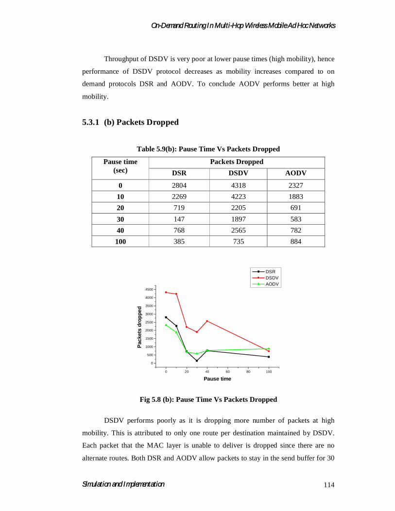
5.3.1 (b) Packets Dropped
Table 5.9(b): Pause Time Vs Packets Dropped
Pause time(sec)
Packets Dropped
DSR DSDV AODV
0 2804 4318 2327
10 2269 4223 1883
20 719 2205 691
30 147 1897 583
40 768 2565 782
100 385 735 884
0 20 40 60 80 100
0
500
1000
1500
2000
2500
3000
3500
4000
4500
Pac
kets
dro
pp
ed
DSR DSDV AODV
Pause time
Fig 5.8 (b): Pause Time Vs Packets Dropped
DSDV performs poorly as it is dropping more number of packets at high
mobility. This is attributed to only one route per destination maintained by DSDV.
Each packet that the MAC layer is unable to deliver is dropped since there are no
alternate routes. Both DSR and AODV allow packets to stay in the send buffer for 30

On-Demand Routing In Multi-Hop Wireless Mobile Ad Hoc Networks
Simulation and Implementation 115
seconds for route discovery and once the route is discovered, data packets are sent on
that route to be delivered at the destination. If route fails, both DSR and AODV find
new path within 30 seconds there by minimizing the possibility of packet drop.
5.3.1 (c) Packet Delivery ratio
Table 5.9(c): Pause Time Vs Packet Delivery Ratio
Pause time(sec)
Packet Delivery Ratio
DSR DSDV AODV
0 0.8324 0.71163 0.84454
10 0.84911 0.71792 0.87416
20 0.952 0.85261 0.95403
30 0.99019 0.87292 0.96122
40 0.94869 0.82849 0.94776
100 0.97698 0.95096 0.94131
0 20 40 60 80 100
0.70
0.72
0.74
0.76
0.78
0.80
0.82
0.84
0.86
0.88
0.90
0.92
0.94
0.96
0.98
1.00
DSR DSDV AODV
Pac
ket
del
ivar
y ra
tio
Pause time
Fig 5.8 (c): Pause Time Vs Packet Delivery Ratio
Packet delivery ratio of DSDV is very less as compared to on demand
protocols DSR and AODV at lower pause time (high mobility). AODV and DSR
perform best among all at high mobility. The reason for having better packet delivery
ratio of DSR and AODV is that both allow packets to stay in the send buffer for 30

On-Demand Routing In Multi-Hop Wireless Mobile Ad Hoc Networks
Simulation and Implementation 116
seconds for route discovery and once the route is discovered, data packets are sent on
that route to be delivered at the destination.
5.3.1 (d) Routing overhead
Table 5.9 (d): Pause Time Vs Routing Overhead
Pause time(sec)
Routing overhead
DSR DSDV AODV
0 65.438 70.6464 59.64725
10 70.65239 74.4132 63.53916
20 39.37512 56.57754 45.20056
30 43.4977 57.45847 53.69828
40 49.81964 51.58809 49.5791
100 61.36803 71.70136 68.25334
0 20 40 60 80 10035
40
45
50
55
60
65
70
75
DSR DSDV AODV
Ro
uti
ng
ove
rhea
d
Pause time
Fig 5.8 (d): Pause Time Vs Routing Overhead
DSDV uses the table-driven approach of maintaining routing information. It is
not as adaptive to the route changes that occur during high mobility. DSDV sends
periodic routing updates at every 15 seconds in the network. These periodic
broadcasts increase routing load in the network. Hence DSDV results in to more
routing overhead irrespective of mobility. For longer duration pause as DSDV sends
periodic updates at regular intervals. AODV and DSR build the routing information as
On-Demand Routing In Multi-Hop Wireless Mobile Ad Hoc Networks
Simulation and Implementation 117
and when they are needed. This results in better performance (high packet delivery
fraction) and less routing load. DSR works better at moderate mobility of nodes where
as AODV is works better even at high mobility.
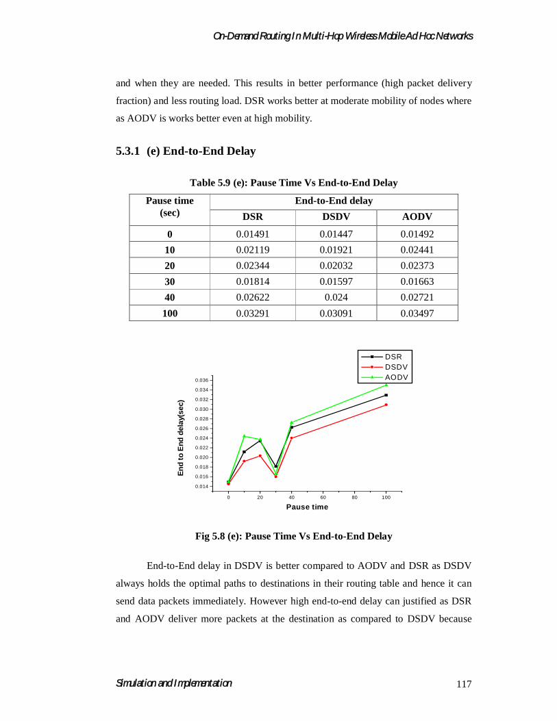
5.3.1 (e) End-to-End Delay
Table 5.9 (e): Pause Time Vs End-to-End Delay
Pause time(sec)
End-to-End delay
DSR DSDV AODV
0 0.01491 0.01447 0.01492
10 0.02119 0.01921 0.02441
20 0.02344 0.02032 0.02373
30 0.01814 0.01597 0.01663
40 0.02622 0.024 0.02721
100 0.03291 0.03091 0.03497
0 20 40 60 80 100
0.014
0.016
0.018
0.020
0.022
0.024
0.026
0.028
0.030
0.032
0.034
0.036
DSR DSDV AODV
En
d t
o E
nd
del
ay(s
ec)
Pause time
Fig 5.8 (e): Pause Time Vs End-to-End Delay
End-to-End delay in DSDV is better compared to AODV and DSR as DSDV
always holds the optimal paths to destinations in their routing table and hence it can
send data packets immediately. However high end-to-end delay can justified as DSR
and AODV deliver more packets at the destination as compared to DSDV because

On-Demand Routing In Multi-Hop Wireless Mobile Ad Hoc Networks
Simulation and Implementation 118
these two protocols try to provide some sort of guarantee for the packets to be
delivered at the destination by compromising at the cost of delay.
5.3.1 (f) Optimal Path Length
Table 5.9 (f): Pause Time Vs Optimal Path Length
Pause time(sec)
Optimal Path Length
DSR DSDV AODV
0 1.78614 1.43065 1.70627
10 1.83208 1.47934 1.72686
20 1.4136 1.31172 1.47378
30 1.43929 1.31456 1.55865
40 1.52514 1.38128 1.52312
100 1.62813 1.54367 1.72509
0 20 40 60 80 100
1.3
1.4
1.5
1.6
1.7
1.8
1.9 DSR DSDV AODV
Op
tim
al p
ath
len
gth
Pause time
Fig 5.8 (f): Pause Time Vs Optimal Path Length
Optimal path varies as the pause time (mobility) varies. DSDV performs better
in terms of optimal path irrespective of variation in mobility as the nodes in DSDV
always hold the optimal path to every other destination in their routing tables and the
routing table is periodically updating.

On-Demand Routing In Multi-Hop Wireless Mobile Ad Hoc Networks
Simulation and Implementation 119
5.3.2 Simulation Results: THE EFFECT OF TRAFFIC LOAD
To study the effect of traffic load on the network, number of connections was
varied as 10, 20, 30 and 40 connections. The network was simulated for high mobility
scenario keeping the pause time 0 seconds. Graphs in Fig 5.9 (a-f) show the effect
Traffic Load for DSDV, DSR and AODV protocols with respect to various
performance metrics.
5.3.2 (a) Throughput
Table 5.10 (a): Max. Number of Connections Vs Throughput (Bits/Sec)
Max. Number of
Connections
Throughput
DSR DSDV AODV
10 6031 5033 6015
20 10299 7937 10223
30 12471 10656 12641
40 13070 12067 13354
10 15 20 25 30 35 404000
5000
6000
7000
8000
9000
10000
11000
12000
13000
14000
D S R D S D V A O D V
Th
rou
gh
pu
t(b
its/
sec)
M ax.N um ber of connections
Fig 5.9 (a): Max. Number of Connections Vs Throughput (bits/Sec)
As the traffic load increases both on-demand protocols work better compared
to DSDV. Throughput of AODV is high at higher traffic load where as DSR performs
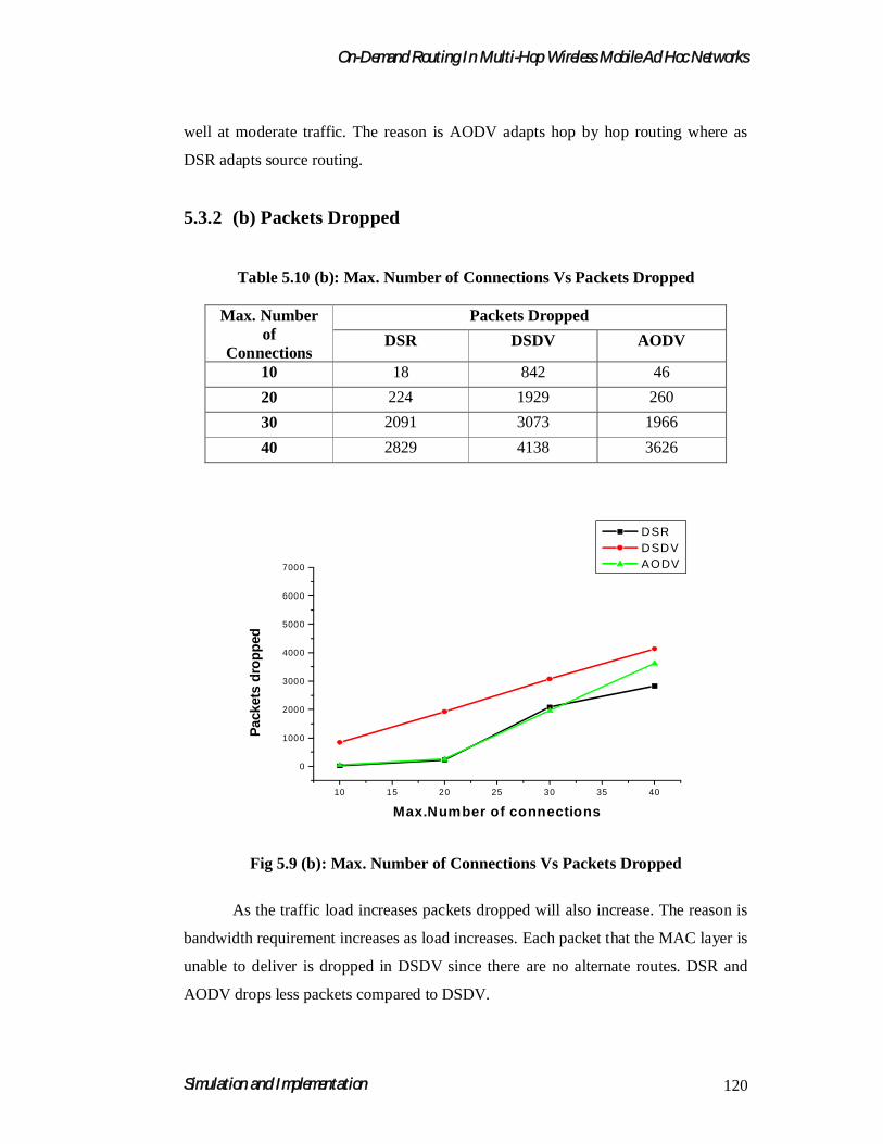
On-Demand Routing In Multi-Hop Wireless Mobile Ad Hoc Networks
Simulation and Implementation 120
well at moderate traffic. The reason is AODV adapts hop by hop routing where as
DSR adapts source routing.
5.3.2 (b) Packets Dropped
Table 5.10 (b): Max. Number of Connections Vs Packets Dropped
Max. Number of
Connections
Packets Dropped
DSR DSDV AODV
10 18 842 46
20 224 1929 260
30 2091 3073 1966
40 2829 4138 3626
10 15 20 25 30 35 40
0
1000
2000
3000
4000
5000
6000
7000
DSR DSDV AODV
Pac
kets
dro
pp
ed
Max.Number of connections
Fig 5.9 (b): Max. Number of Connections Vs Packets Dropped
As the traffic load increases packets dropped will also increase. The reason is
bandwidth requirement increases as load increases. Each packet that the MAC layer is
unable to deliver is dropped in DSDV since there are no alternate routes. DSR and
AODV drops less packets compared to DSDV.
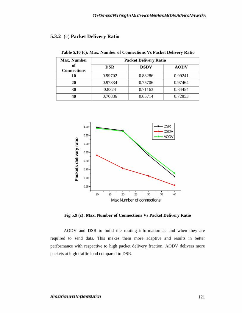
On-Demand Routing In Multi-Hop Wireless Mobile Ad Hoc Networks
Simulation and Implementation 121
5.3.2 (c) Packet Delivery Ratio
Table 5.10 (c): Max. Number of Connections Vs Packet Delivery Ratio
Max. Number of
Connections
Packet Delivery Ratio
DSR DSDV AODV
10 0.99702 0.83286 0.99241
20 0.97834 0.75706 0.97464
30 0.8324 0.71163 0.84454
40 0.70836 0.65714 0.72853
10 15 20 25 30 35 40
0.65
0.70
0.75
0.80
0.85
0.90
0.95
1.00 DSR DSDV AODV
Pac
kets
del
ivar
y ra
tio
Max.Number of connections
Fig 5.9 (c): Max. Number of Connections Vs Packet Delivery Ratio
AODV and DSR to build the routing information as and when they are
required to send data. This makes them more adaptive and results in better
performance with respective to high packet delivery fraction. AODV delivers more
packets at high traffic load compared to DSR.

On-Demand Routing In Multi-Hop Wireless Mobile Ad Hoc Networks
Simulation and Implementation 122
5.3.2 (d) Routing Overhead
Table 5.10 (d): Max. Number of Connections Vs Routing Overhead
Max. Number of
Connections
Routing Overhead
DSR DSDV AODV
10 31.60853 67.5906 55.89837
20 73.98119 87.03739 82.86777
30 65.43853 70.64645 59.64725
40 58.88028 64.5657 47.21768
10 15 20 25 30 35 40
30
40
50
60
70
80
90 DSR DSDV AODV
Ro
uti
ng
ove
rhea
d
Max.Number of connections
Fig 5.9 (d): Max. Number of Connections Vs Routing Overhead
Periodic broadcasts of control packets of DSDV increase routing load in the
network and hence DSDV has more routing overhead irrespective traffic load. Further
this worsens with increasing number of node. Even under stand still condition of
network DSDV keeps on sending periodic updates at regular intervals among the
nodes. AODV performs better at high traffic since it computes route as and when
needed and it adapts hop-by-hop routing. However DSR performs better at low and
moderate sized traffic load because it uses source routing and the length of packet
header will not be too large at low and moderate sized traffic.
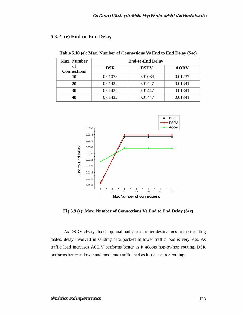
On-Demand Routing In Multi-Hop Wireless Mobile Ad Hoc Networks
Simulation and Implementation 123
5.3.2 (e) End-to-End Delay
Table 5.10 (e): Max. Number of Connections Vs End to End Delay (Sec)
Max. Number of
Connections
End-to-End Delay
DSR DSDV AODV
10 0.01073 0.01064 0.01237
20 0.01432 0.01447 0.01341
30 0.01432 0.01447 0.01341
40 0.01432 0.01447 0.01341
10 15 20 25 30 35 40
0.0105
0.0110
0.0115
0.0120
0.0125
0.0130
0.0135
0.0140
0.0145
0.0150
DSR DSDV AODV
En
d t
o E
nd
del
ay
Max.Number of connections
Fig 5.9 (e): Max. Number of Connections Vs End to End Delay (Sec)
As DSDV always holds optimal paths to all other destinations in their routing
tables, delay involved in sending data packets at lower traffic load is very less. As
traffic load increases AODV performs better as it adopts hop-by-hop routing. DSR
performs better at lower and moderate traffic load as it uses source routing.
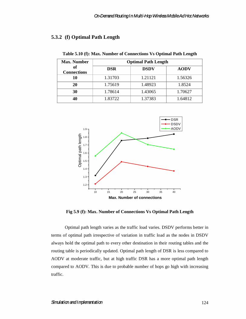
On-Demand Routing In Multi-Hop Wireless Mobile Ad Hoc Networks
Simulation and Implementation 124
5.3.2 (f) Optimal Path Length
Table 5.10 (f): Max. Number of Connections Vs Optimal Path Length
Max. Number of
Connections
Optimal Path Length
DSR DSDV AODV
10 1.31703 1.21121 1.56326
20 1.75619 1.48923 1.8524
30 1.78614 1.43065 1.70627
40 1.83722 1.37383 1.64812
10 15 20 25 30 35 40
1.2
1.3
1.4
1.5
1.6
1.7
1.8
1.9
Opt
imal
pat
h le
ngth
DSR DSDV AODV
Max. Number of connections
Fig 5.9 (f): Max. Number of Connections Vs Optimal Path Length
Optimal path length varies as the traffic load varies. DSDV performs better in
terms of optimal path irrespective of variation in traffic load as the nodes in DSDV
always hold the optimal path to every other destination in their routing tables and the
routing table is periodically updated. Optimal path length of DSR is less compared to
AODV at moderate traffic, but at high traffic DSR has a more optimal path length
compared to AODV. This is due to probable number of hops go high with increasing
traffic.
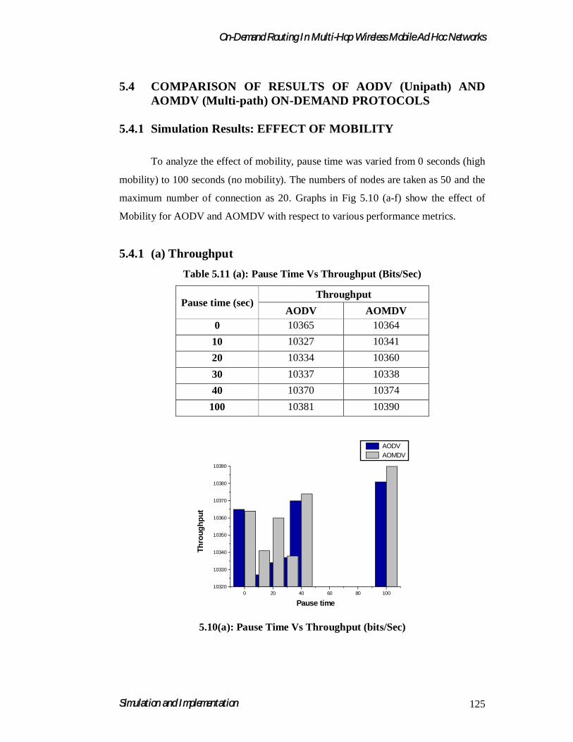
On-Demand Routing In Multi-Hop Wireless Mobile Ad Hoc Networks
Simulation and Implementation 125
5.4 COMPARISON OF RESULTS OF AODV (Unipath) AND AOMDV (Multi-path) ON-DEMAND PROTOCOLS
5.4.1 Simulation Results: EFFECT OF MOBILITY
To analyze the effect of mobility, pause time was varied from 0 seconds (high
mobility) to 100 seconds (no mobility). The numbers of nodes are taken as 50 and the
maximum number of connection as 20. Graphs in Fig 5.10 (a-f) show the effect of
Mobility for AODV and AOMDV with respect to various performance metrics.
5.4.1 (a) Throughput
Table 5.11 (a): Pause Time Vs Throughput (Bits/Sec)
Pause time (sec)Throughput
AODV AOMDV0 10365 10364
10 10327 10341
20 10334 10360
30 10337 10338
40 10370 10374
100 10381 10390
0 20 40 60 80 10010320
10330
10340
10350
10360
10370
10380
10390
AODV AOMDV
Th
rou
gh
pu
t
Pause time
5.10(a): Pause Time Vs Throughput (bits/Sec)

On-Demand Routing In Multi-Hop Wireless Mobile Ad Hoc Networks
Simulation and Implementation 126
Due to several inherent properties of AOMDV like Load Balancing and Bandwidth
Aggregation, AOMDV always outperforms AODV. When a link becomes over
utilized and causes congestion, AOMDV can choose to divert traffic through alternate
paths and hence throughput increases.
5.4.1 (b) Packets dropped
Table 5.11(b): Pause Time Vs Packets Dropped
Pause time (sec)Packets Dropped
AODV AOMDV0 83 7
10 95 37
20 97 48
30 124 54
40 118 52
100 150 65
0 20 40 60 80 1000
20
40
60
80
100
120
140
160
Pac
kets
dro
pp
ed
Pause time
AODV AOMDV
Fig 5.10 (b): Pause Time Vs Packets Dropped
The packet dropped varies with mobility. Number of packets dropped in
AOMDV is always less compared to AODV. Multipath nature of AOMDV attributes
to less packet drop.

On-Demand Routing In Multi-Hop Wireless Mobile Ad Hoc Networks
Simulation and Implementation 127
5.4.1 (c) Packet delivery ratio
Table 5.11 (c): Pause Time Vs Packet Delivery Ratio
Pause time (sec)Packet Delivery Ratio
AODV AOMDV0 0.99083 0.99933
10 0.97428 0.99371
20 0.97116 0.99419
30 0.96424 0.99478
40 0.96899 0.99643
100 0.96812 0.99538
0 20 40 60 80 1000.960
0.965
0.970
0.975
0.980
0.985
0.990
0.995
1.000
AODV AOMDV
Pac
ket
del
iver
y ra
tio
Pause time
Fig 5.10 (c): Pause Time Vs Packet Delivery Ratio
Packet delivery ratio in AOMDV is always more, due to availability of
multiple paths as compared to AODV irrespective of variation in mobility. When a
link becomes over utilized resulting into congestion or failures, multipath routing
protocols can divert traffic through alternate paths.

On-Demand Routing In Multi-Hop Wireless Mobile Ad Hoc Networks
Simulation and Implementation 128
5.4.1 (d) Routing overhead
Table 5.11 (d): Pause Time Vs Routing Overhead
Pause time (sec)Routing Overhead
AODV AOMDV0 58.54317 47.7035
10 53.78135 34.9192
20 76.5047 42.25949
30 49.3753 32.9054
40 57.29026 39.7949
100 97.377 84.4294
0 20 40 60 80 1000
20
40
60
80
100
Ro
uti
ng
ove
rhea
d
Pause time
AODV AOMDV
Fig 5.10 (d): Pause Time Vs Routing Overhead
Routing overhead in AOMDV is less compared to AODV, because the
frequency of route discovery is less in AOMDV as multiple routes are always
available. New route discovery is needed only when the entire link-disjoint paths fails.
The probability such situation is very less.

On-Demand Routing In Multi-Hop Wireless Mobile Ad Hoc Networks
Simulation and Implementation 129
5.4.1 (e) End-to-End Delay (sec)
Table 5.11(e): Pause Time Vs End-to-End Delay (Sec)
Pause time (sec)End-to-End Delay (Sec)
AODV AOMDV0 0.12441 0.10382
10 0.11663 0.10363
20 0.23725 0.20435
30 0.11663 0.10295
40 0.11721 0.10351
100 0.13097 0.10017
0 20 40 60 80 1000.00
0.05
0.10
0.15
0.20
0.25
End
to
End
del
ay(s
ec)
Pause time
AODV AOMDV
Fig 5.10 (e): Pause Time Vs End-to-End Delay
AOMDV protocol is designed to adopt multiple paths architecture of network,
which is a step towards achieving a high QoS, and hence delay involved in sending a
data packets is less compared to AODV.

On-Demand Routing In Multi-Hop Wireless Mobile Ad Hoc Networks
Simulation and Implementation 130
5.4.1 (f) Optimal path length
Table 5.11 (f): Pause Time Vs Optimal Path Length
Pause time (sec)Optimal Path Length
AODV AOMDV0 1.58583 1.48144
10 1.54122 1.3778
20 1.46951 1.34918
30 1.49616 1.41497
40 1.5749 1.45877
100 1.97775 1.88195
0 20 40 60 80 1001.3
1.4
1.5
1.6
1.7
1.8
1.9
2.0
AODV AOMDV
Opt
imal
pat
h le
ngth
Pause time
Fig 5.10 (f): Pause Time Vs Optimal Path Length
The optimal path length in terms of number of hops present across the optimal
path is less in AOMDV irrespective of variations in mobility (pause time). Because of
existence of multiple paths, option remains open for selecting a best optimal path.
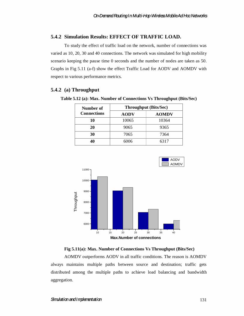
On-Demand Routing In Multi-Hop Wireless Mobile Ad Hoc Networks
Simulation and Implementation 131
5.4.2 Simulation Results: EFFECT OF TRAFFIC LOAD.
To study the effect of traffic load on the network, number of connections was
varied as 10, 20, 30 and 40 connections. The network was simulated for high mobility
scenario keeping the pause time 0 seconds and the number of nodes are taken as 50.
Graphs in Fig 5.11 (a-f) show the effect Traffic Load for AODV and AOMDV with
respect to various performance metrics.
5.4.2 (a) Throughput
Table 5.12 (a): Max. Number of Connections Vs Throughput (Bits/Sec)
Number of Connections
Throughput (Bits/Sec)
AODV AOMDV10 10065 10364
20 9065 9365
30 7065 7364
40 6006 6317
10 15 20 25 30 35 40
6000
7000
8000
9000
10000
11000
AODV AOMDV
Th
rou
ghpu
t
Max.Number of connections
Fig 5.11(a): Max. Number of Connections Vs Throughput (Bits/Sec)
AOMDV outperforms AODV in all traffic conditions. The reason is AOMDV
always maintains multiple paths between source and destination; traffic gets
distributed among the multiple paths to achieve load balancing and bandwidth
aggregation.
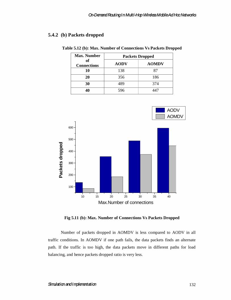
On-Demand Routing In Multi-Hop Wireless Mobile Ad Hoc Networks
Simulation and Implementation 132
5.4.2 (b) Packets dropped
Table 5.12 (b): Max. Number of Connections Vs Packets Dropped
Max. Number of
Connections
Packets Dropped
AODV AOMDV
10 138 87
20 356 186
30 489 374
40 596 447
10 15 20 25 30 35 40
100
200
300
400
500
600
AODV AOMDV
Pac
kets
dro
pp
ed
Max.Number of connections
Fig 5.11 (b): Max. Number of Connections Vs Packets Dropped
Number of packets dropped in AOMDV is less compared to AODV in all
traffic conditions. In AOMDV if one path fails, the data packets finds an alternate
path. If the traffic is too high, the data packets move in different paths for load
balancing, and hence packets dropped ratio is very less.

On-Demand Routing In Multi-Hop Wireless Mobile Ad Hoc Networks
Simulation and Implementation 133
5.4.2 (c) Packet delivery ratio
Table 5.12 (c): Max. Number of Connections Vs Packet Delivery Ratio
Max. Number of
Connections
Packet Delivery Ratio
AODV AOMDV
10 0.98637 0.99917
20 0.96083 0.97933
30 0.93083 0.94933
40 0.91083 0.92933
10 15 20 25 30 35 400.90
0.91
0.92
0.93
0.94
0.95
0.96
0.97
0.98
0.99
1.00
AODV AOMDV
Pac
ket
del
iver
y ra
tio
Max.Number of connections
Fig 5.11 (c): Max. Number of Connections Vs Packet Delivery Ratio
Packet delivery ratio in AOMDV is more, as multiple paths for data transfer
are always available as compared to AODV irrespective of variation in traffic load.
Traffic gets distributed among different paths as the load exceeds the capacity of
paths and achieves load balancing and bandwidth sharing.

On-Demand Routing In Multi-Hop Wireless Mobile Ad Hoc Networks
Simulation and Implementation 134
5.4.2 (d) Routing Overhead
Table 5.12 (d): Max. Number of Connections Vs Routing Overhead
Max. Number of
Connections
Routing Overhead
AODV AOMDV
10 45.3534 43.3438
20 48.5431 45.7035
30 50.5431 47.7035
40 58.5431 49.7035
10 15 20 25 30 35 4042
44
46
48
50
52
54
56
58
60
AODV AOMDV
Ro
uti
ng
ove
rhea
d
Max.Number of connections
Fig 5.11 (d): Max. Number of Connections Vs Routing Overhead
Routing overhead in AOMDV is low compared to AODV. Because the
frequency of route discovery is less in AOMDV as if one path fails or congested, an
alternate path is utilized to divert packets and hence new route discovery is needed
only when the entire link paths fails.

On-Demand Routing In Multi-Hop Wireless Mobile Ad Hoc Networks
Simulation and Implementation 135
5.4.2 (e) End-to-End Delay (sec)
Table 5.12(f): Max. Number of Connections Vs End-to-End Delay
Max. Numberof
Connections
End-to-End Delay
AODV AOMDV
10 0.01237 0.0104
20 0.01941 0.01182
30 0.02141 0.01282
40 0.02441 0.01482
5 10 15 20 25 30 35 40 450.000
0.005
0.010
0.015
0.020
0.025
End
to E
nd d
ela
y(se
c)
Max.Number of connections
AODV AOMDV
Fig 5.11 (e): Max. Number of Connections Vs End to End Delay.
AOMDV protocol designed to adopt multiple paths architecture of network,
which is a step towards achieving a better QoS, and hence end to end delay involved
in sending a data packets is less compared to AODV irrespective of variation in traffic
load.

On-Demand Routing In Multi-Hop Wireless Mobile Ad Hoc Networks
Simulation and Implementation 136
5.4.2 (f) Optimal Path Length
Table 5.12 (f): Max. Number of Connections Vs Optimal Path Length
Max. Number of
Connections
Optimal Path Length
AODV AOMDV
10 1.45391 1.43943
20 1.57583 1.47815
30 1.58583 1.48815
40 1.59858 1.49815
.
10 15 20 25 30 35 40
1.44
1.46
1.48
1.50
1.52
1.54
1.56
1.58
1.60
1.62
AODV AOMDV
Opt
imal
pat
h le
ngth
Max. Number of connections
Fig 5.11 (f): Max. Number of Connections Vs Optimal Path Length
The optimal path length in terms of number of hops present across the route
between sauce and destination is less in AOMDV irrespective of variations in traffic
load due to availability of best optimal paths among the multiple paths in AOMDV.

On-Demand Routing In Multi-Hop Wireless Mobile Ad Hoc Networks
Simulation and Implementation 137
5.5 SUMMERY OF RESULT ANALYSIS
The simulation results have demonstrated some important characteristic
differences among the various routing protocols. The presence of high mobility
implies frequent link failures and each routing protocol reacts differently during link
failures. The different basic working mechanism of these protocols leads to the
differences in the performance. DSDV fails to converge at lower pause time, hence
performance of the protocol decreases as mobility increases. At higher rates of
mobility (lower pause times), DSDV performs poorly dropping more number of
packets. As DSDV maintains only one route per destination, each packet that the
MAC layer is unable to deliver is dropped since there are no alternate routes. For DSR
and AODV, packet delivery ratio is independent of offered traffic load, with both
protocols delivering between 82% and 100% of the packets in all cases. The reason
for having better packet delivery ratio of DSR and AODV is that both allow packets
to stay in the send buffer for 30 seconds for route discovery and once the route is
discovered, data packets are sent on that route to be delivered at the destination. It is
observed that the DSR and AODV deliver more packets at the destination as
compared to DSDV because these two protocols try to provide some sort of guarantee
for the packets to be delivered at the destination by compromising at the cost of delay,
where as for DSDV if it is not possible to deliver a packet it tries to drop it. This
accounts for smaller delay and lesser packet delivery ratio.
DSDV uses the table-driven approach of maintaining routing information. It is
not as adaptive to the route changes that occur during high mobility. DSDV sends
periodic routing updates at every 15 seconds in the network. These periodic
broadcasts increase routing load in the network. Hence DSDV is imposed with high
routing overhead irrespective of mobility and traffic load. If network exists for longer
period, overhead further increases as the DSDV sends periodic updates at regular
interval.
In contrast, the lazy approach used by the on-demand protocols, AODV and
DSR to build the routing information as and when they are needed which make them
more adaptive and results in better performance (high packet delivery fraction) and
less routing load. DSR works better at moderate mobility of nodes (as it adapts source

On-Demand Routing In Multi-Hop Wireless Mobile Ad Hoc Networks
Simulation and Implementation 138
routing) where as AODV works better at high mobility and high traffic load (as it
adapts hop-by-hop routing).
Both DSR and AODV are unipath on demand routing protocols. A more
recent research topic for MANETs could be multipath routing protocols. Multipath
routing protocols establish multiple disjoint paths from a source to a destination and
are thereby improving resilience to network failures and allows network for load
balancing. These effects are particularly interesting in networks with high node
density (and the corresponding larger choice of disjoint paths) and high network load
(due to the ability to load balance the traffic around congested networks). The benefits
of multipath routing protocol are fault tolerance, load balancing, bandwidth
aggregation and reduced End-to-End delay.
Overall analysis of results indicate that for a network with low mobility and
less number of nodes, DSDV is preferable. Investigation also suggests that the
performance of DSR which uses source routing is preferable for the normal network
of general nature with moderate traffic and moderate mobility as it delivers more
packets at the destination with lowest routing overheads. For robust scenario where
mobility is high, nodes are dense, area is large, the amount of traffic is more and
network pattern sustains for longer period, AODV performs better. To achieve lower
routing overhead, better throughput, lower end-to-end delay, to be more resilient to
route failures and alleviate congestion for robust scenario where mobility is high,
nodes are dense and traffic is more, AOMDV is the best choice.
The overall conclusion is that a multipath routing protocol, AOMDV is best
choice to move towards a network with better Quality of Service (QoS).