Chapter 5 Multispectral, thermal and hyperspectral scanning Introduction to Remote Sensing...

Chapter 5Chapter 5

Multispectral, thermal and Multispectral, thermal and hyperspectral scanninghyperspectral scanning

Introduction to Remote SensingInstructor: Dr. Cheng-Chien Liu

Department of Earth Sciences

National Cheng-Kung University

Last updated: 7 May 2003

5.15.1 Introduction Introduction

MSS (multispectral scanning) vs. MCS MSS (multispectral scanning) vs. MCS (Multiband camera system)(Multiband camera system)• Fig 2.42, 2.43 (MCS)

• AdvantagesSpectral bands: 0.3~1.4 m with narrow band widthCollection: same optical system for all bands.Calibration: electronically rather than photochemically.Storage and transmission

5.2 Across-track multispectral 5.2 Across-track multispectral scanningscanning

Across-track (whiskbroom) scanner:Across-track (whiskbroom) scanner:• Fig 5.1: operation of a five-channels sensor flight line• Using a rotating or oscillating mirror (Fig 5.1b)• Contiguous strips 2D image• Dichroic grating two forms of energy

ThermalNonthermal prism UV, Vis and near-IR

• Detectors spectral sensitivity• Signal amplified recorded A-to-D View-in-

flight storage interpretation

5.2 Across-track multispectral 5.2 Across-track multispectral scanning (cont.)scanning (cont.)

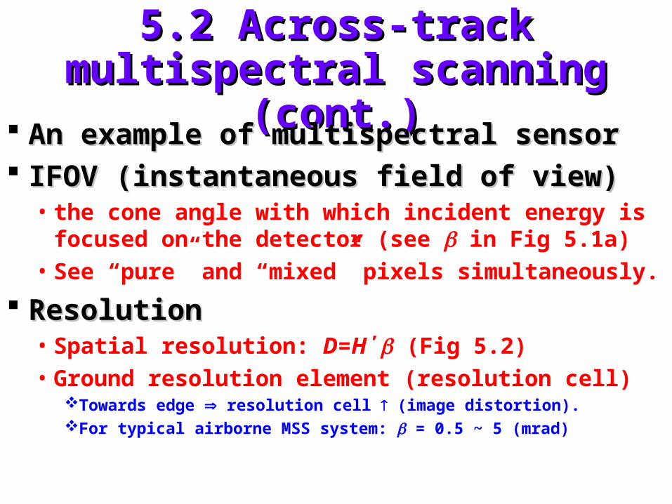
An example of multispectral sensorAn example of multispectral sensor IFOV (instantaneous field of view)IFOV (instantaneous field of view)

• the cone angle with which incident energy is focused on the detector (see in Fig 5.1a)

• See “pure” and “mixed” pixels simultaneously.

ResolutionResolution• Spatial resolution: D=H΄ (Fig 5.2)• Ground resolution element (resolution cell)

Towards edge resolution cell (image distortion).For typical airborne MSS system: = 0.5 ~ 5 (mrad)


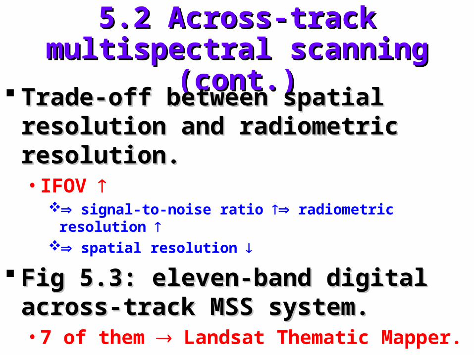
Trade-off between spatial resolution Trade-off between spatial resolution and radiometric resolution.and radiometric resolution.• IFOV

signal-to-noise ratio radiometric resolution spatial resolution

Fig 5.3: eleven-band digital across-Fig 5.3: eleven-band digital across-track MSS system.track MSS system.• 7 of them Landsat Thematic Mapper.


Fig 5.4: eleven-band MSS imagesFig 5.4: eleven-band MSS images• (A) street (B) grass:

clear contrast in all bandsTonal reversal: from band 8~10 (near-IR)

• (C) water (B) grass: difficult to differentiate in the Vis-band, but clean contrast

in near-IR bands.

• (D) cloud shadow:channel 1:somewhat illuminated by Rayleigh scatter near-IR low Rayleigh scatter darkest thermal no signal (moving clouds)


Fig 5.5: eight-band MSS imageFig 5.5: eight-band MSS image• Pavement grass:

clear in Vis-band(1~3)tones reverse in near-IR(4, 5) and mid-IR (6, 7)

• River plume: clear in thermal band (8)

• Dock: clear in band (6~8)

5.3 Along-track multispectral 5.3 Along-track multispectral scanningscanning

Along-track (pushbroom) scannerAlong-track (pushbroom) scanner• Fig 5.6

• A linear array of CCDs (charge-coupled device)

No scanning mirrorSize of detectors ground resolution

The smaller the better

Each band one array

5.3 Along-track multispectral 5.3 Along-track multispectral scanning (cont.)scanning (cont.)

Along-track (pushbroom) scanner (cont.)Along-track (pushbroom) scanner (cont.)• Pros:

Longer dwell time (residence time) Stronger and greater range of signal Better spatial and radiometric resolution

Fixed detector geometric integrity Size & weight & power No moving part reliability & life expectancy

• Cons:CalibrationLimited range of spectral sensitivity (<near –IR)

Underdeveloping


Fig 5.7 MEIS IIFig 5.7 MEIS II• the first airborne pushbroom scanner

• 1728-element linear arrays

• 8 spectral bands (0.39 m~1.1 m)

• IFOV 0.7 m rad

TFOV 400

• 8-bit (256 DN)


Fig 5.8: MEIS II in stereomode.Fig 5.8: MEIS II in stereomode.• External mirror forward-looking & aft-

looking

MOMS ( the 1MOMS ( the 1stst space borne space borne pushbroom scanner)pushbroom scanner)

5.4 Across-track thermal scanning5.4 Across-track thermal scanning

Thermal portion of the spectrumThermal portion of the spectrum• Atmospheric window two ranges (3~5m,

8~14 m)

Rapid response (<1-Rapid response (<1-sec)sec)• Photon electrical charge• Dewar cool detector

3 photon detectors in common use 3 photon detectors in common use todaytoday• Table 5.1: spectral sensitivity range

5.4 Across-track thermal scanning 5.4 Across-track thermal scanning (cont.)(cont.)

Fig 5.9Fig 5.9• Across-track thermal scanner schematic• Recording procedure:

1. Incoming energy2. Additional optics3. Focusing detector4. Detector (encased by a dewar) signal5. Amplify6. Display &record, amplified signal modulate tube7. Scan8. Record

• Platen• Film advanced rate = fn(V/H΄)• Fig 5.10: a typical thermal scanner system

5.5 Thermal radiation principles5.5 Thermal radiation principles

Radiant versus kinetic temperatureRadiant versus kinetic temperature• Kinetic temperature: contact internal

manifestation average translational energy of the molecules

• Radiant temperature: emitted energy external manifestation object’s energy state

Blackbody radiationBlackbody radiation• Fig 5.11: Spectral distribution of energy radiated

from blackbodies of various temperatures• Wien’s displacement law• Stefan-Boltzmann law

5.5 Thermal radiation principles 5.5 Thermal radiation principles (cont.)(cont.)

Radiation from real materialsRadiation from real materials• No perfect blackbody• Emissivity: (T) Mreal(T) / Mblack body(T)

0 < < 1fn(, viewing, T)

• Graybody fn(• Selective radiator = fn(

Fig 5.12 Fig 5.13: (6~14m)

Water ~ blackbody ( Quartz ~ selective radiator


Radiation from real materials (cont.)Radiation from real materials (cont.)• Importance of M( = 8~14 m) thermal sensing

Atmospheric windowM(T=300K) = 9.7 mFor broadband sensor treated as graybodyTable 5.2: typical values of emissivity over 8~14 m

Atmospheric effectsAtmospheric effects• Atmospheric windows: Fig 5.14

Thermal range : (3~5 m, 8~14 m)Atmospheric absorption & scattering colder objects.

Atmospheric emission warmer objectBiased sensor outputCompensation later this chapter


Interaction of thermal radiation with terrain Interaction of thermal radiation with terrain elements.elements.• EI=EA+ER+ET conservation of energy.

1 = ++ normalize1 = ++ Kirchhoff radiation law (good absorbersgood emitters)1= + assumption of opaque to thermal radiation.

• For real body:M= T4

Trad=Tkin

Table 5.3: typical valuesAlways underestimate T if neglect effect

• Surface T (<50m) internal bulk T

5.6 Interpreting thermal scanner 5.6 Interpreting thermal scanner imageryimagery

Successful interpretationsSuccessful interpretations• Rock type, structure• Locating geologic faults• Mapping soil type & moisture• Locating irrigation canal leaks.• Volcanoes.• Evapo-transpiration from vegetation.• Locating cold water springs.• Locating hot water springs & geysers.• Thermal plumes in lakes and rivers.• Natural circulation patterns in water bodies.• Forest fires.• Locating subsurface fires in landfills or coal refuse piles

5.6 Interpreting thermal scanner 5.6 Interpreting thermal scanner imagery (cont.)imagery (cont.)

Most application Most application qualitativequalitative

Some application Some application quantitative quantitative Considerations of the time for acquiring thermal Considerations of the time for acquiring thermal

datadata• Fig 5.15: generalized diurnal radiant T variations.

Water range of T is small

Water Tmax(water) Tmax(rock)+1~2Crossovers

• Thermal conductivity• Thermal capacity• Thermal inertia ( conductivity)

• Predawn imagery preferred but difficult


Fig 5.16: day time and night time imageryFig 5.16: day time and night time imagery• Water

• Land

• Trees

• Paved area

Fig 5.17: day time thermal imageryFig 5.17: day time thermal imagery• Beach ridge(B)

• Lakebed soil(A)

• Trees( C )

• Bare soil (D)

• Mowed grass (E)


Fig 5.18: night time thermal imageryFig 5.18: night time thermal imagery• Cows• Deers• Metal roof

Fig 5.19: high resolution daytime thermal Fig 5.19: high resolution daytime thermal imageimage• Helicopter shadows

Fig 5.20: Daytime thermal imageryFig 5.20: Daytime thermal imagery• Hot water• Circulations


Fig 5.21 nighttime thermal image depicting Fig 5.21 nighttime thermal image depicting building heat loss.building heat loss.

Fig 5.22 Thermovision camera and display Fig 5.22 Thermovision camera and display unitunit

Fig 5.23 Thermal images showing Fig 5.23 Thermal images showing streamline heat loss.streamline heat loss.

NASA’s Thermal infrared Multispectral NASA’s Thermal infrared Multispectral Scanner (TIMS).Scanner (TIMS).• Plate 10(a). TIMS image• Plate 10(b). A generalized lithologic map

5.7 Geometric characteristics of 5.7 Geometric characteristics of across-track scanner imageryacross-track scanner imagery

Along-track scanner Along-track scanner no mirror, fixed no mirror, fixed geometric relationshipgeometric relationship

Across-track scanner Across-track scanner systematic and systematic and random geometric variationsrandom geometric variations• Spatial resolution and ground coverage

Table 5.4W= 2H΄tan

5.7 Geometric characteristics of 5.7 Geometric characteristics of across-track scanner imagery (cont.)across-track scanner imagery (cont.)

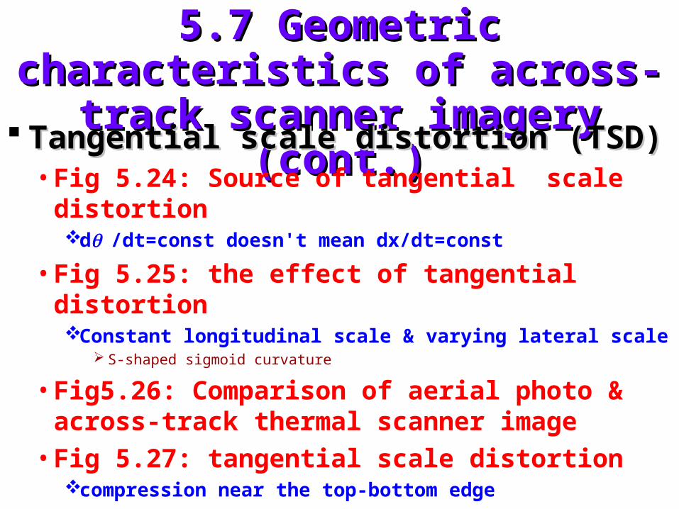
Tangential scale distortion (TSD)Tangential scale distortion (TSD)• Fig 5.24: Source of tangential scale distortion

d/dt=const doesn't mean dx/dt=const

• Fig 5.25: the effect of tangential distortionConstant longitudinal scale & varying lateral scale

S-shaped sigmoid curvature

• Fig5.26: Comparison of aerial photo & across-track thermal scanner image

• Fig 5.27: tangential scale distortioncompression near the top-bottom edge


Tangential scale distortion (cont.)Tangential scale distortion (cont.)• Fig 5.28 correction of TSD

p= ypmax/ymax

Yp= H΄tanp

• Electronically or digitally correct TSD rectilinearized images


Resolution cell size (RCS) variationsResolution cell size (RCS) variations• Fig 5.29

// fight direction H΄ H΄ =H΄sec flight direction H΄ H΄sec=H΄ sec=H΄sec2Response time: time that a scanner takes to respond

electronically to a change in ground reflected or emitted energy

Variations of RCS can be 3~4 times along a scan line

• Limitation of RCS to the image analysisObject>pixel(RCS) representative analysis

• Compensation of irradiance fall-off due to RCS


1-D relief displacement (RD)1-D relief displacement (RD)• Fig 5.30: RD in a vertical aerial photo vs an

across-track scanner image

• Dynamic continuous process sensitive to the aircraft attitude deviations (Fig 5.34)

• Fig 5.31: across-truck thermal scanner image illustrating 1-D RD.


1-D relief displacement (RD)1-D relief displacement (RD)• Fig 5.32: 1-D RD and TSD

• Fig 5.33: Effect of nonsynchronized image recording rate and V/H΄ ratio

• Fig 5.34: distortions induced by aircraft attitude deviations

• Fig 5.35: effect of roll compensation

5.8 Radiometric calibration of 5.8 Radiometric calibration of thermal scannersthermal scanners

Thermal scanner image Thermal scanner image lack of lack of geometric integrity geometric integrity • Take photo simultaneously

• Night time use daytime photo (even old photos will do)

5.8 Radiometric calibration of 5.8 Radiometric calibration of thermal scanners (cont.)thermal scanners (cont.)

Two methods of radiometric calibrationTwo methods of radiometric calibration• Internal blackbody source referencing

Two controlled sources: cold & hotView the sources during every scan lineFig 5.36: configurationA typical mission: height 600m 0.30C but atmospheric condition can

be 20C

• Air-to-ground correlation:Account for atmospheric effectsTheoretical approachEmpirical approach the general approach

Fig 5.37 a sample of calibration curve Fig 5.38 a thermal radiometer used for air-to-ground correlation measurements

5.9 Temperature mapping with 5.9 Temperature mapping with thermal scanner datathermal scanner data

Many applications Many applications MapMap Two proceduresTwo procedures

• Image-basedCrude form: qualitative depiction low geometric and radiometric

integritySuffice for many applicationTonal levels densitometric analysis rectilinerarized imagery.

• Numerically basedN=A+BM=A+BT4

N: DN A, B : to be determined : emissivity T: kinetic temperature

Two unknown (A, B) two equations (data)

5.10 FLIR systems5.10 FLIR systems

Forward-looking infrared (FLIR) Forward-looking infrared (FLIR) system system oblique views of the terrain oblique views of the terrain ahead of an aircraftahead of an aircraft• Fig 5.39

• Point forward sweep across the scene of interest

• Military applications

5.11 Imaging spectrometry5.11 Imaging spectrometry

Hyperspectral Hyperspectral multispectral multispectral• Fig 5.40• Fig 5.41: Selected laboratory spectra of minerals• Hyperspectral data detailed identification of

materials and quantification of their abundance

Airborne Imaging Spectrometer (AIS)Airborne Imaging Spectrometer (AIS)• 128 channel from 1.2~2.4 m with 9.3 nm band width• 1.9 mrad, 4200m high, resolution 8x8m, swath 32 pixel

5.11 Imaging spectrometry (cont.)5.11 Imaging spectrometry (cont.)

Airborne Imaging Spectrometer (cont.)Airborne Imaging Spectrometer (cont.)• Fig 5.42: AIS images

Condominium complexa: schoolb: field

Loss of detail in the atmospheric water absorption band (1.4m) Watered courtyard lawn a (compared to unwatered field b)

Water vapor absorption bands 0.94, 1.14, 1.4, 1.88 m


Fig 5.43: selected laboratory spectra of Fig 5.43: selected laboratory spectra of green leavesgreen leaves• Main components: chlorophyll and water• Shape + peak+valley species

Fig 5.44: same as Fig 5.43 but single speciesFig 5.44: same as Fig 5.43 but single species• Main components: lignin & holocellulose• Difference green or dry holocellulose

Assessing biomassVegetation stressCarbon cycleDiscriminating plant communitiesPhenological conditions


Airborne Visible-Infrared Imaging Airborne Visible-Infrared Imaging Spectrometer (AVIRIS)Spectrometer (AVIRIS)• 224 channels, 0.4~2.45 m with bandwidth 9.6nm• Altitude: 20km, resolution 20m, swath: 10km

• Plate 11: hyperspectral image cubeA common way to display hyperspectral dataColor composite: 0.557(b), 0.815(g), 2.209(r) m

• Fig 5.45Three stages: green leaf initiation development change in plant

pigment proportions flowering domancy leaf loss senescence

• ApplicationsAVIRIS data spectra matching library mineral typeAn export system-based analysis approach


Compact Airborne Spectrographic Compact Airborne Spectrographic Imager (CASI)Imager (CASI)• Commercial, programmable

• 288 channels from 0.4~0.9m with bandwidth 1.8 nm

• IFOV= 1.2 mrad


Geophysical and Environmental Research Geophysical and Environmental Research Imaging Airborne Spectrometer (GERAIS)Imaging Airborne Spectrometer (GERAIS)• 63 channels, 0.4~2.48 m• Fig 5.46: GERAIS Image for identifying minerals

Label A in channel 41 dark spot aluniteAlunite dark from 41~44 absorption light from 49~52 reflection

Red edgeRed edge• The slope of a reflectance spectrum from 0.68~0.76

m• Shift change in the chemical and morphological

status heavy metals in the soil


DIAS-7915DIAS-7915 ASDIS-204ASDIS-204

5.12 Conclusion5.12 Conclusion

Chapter 5 Multispectral, thermal and hyperspectral scanning Introduction to Remote Sensing...

Documents

Transcript of Chapter 5 Multispectral, thermal and hyperspectral scanning Introduction to Remote Sensing...