Response of the Response of the Upper Ocean to Winds Upper Ocean to Winds

Physical oceanographyInstructor: Dr. Cheng-Chien Liu

Department of Earth Sciences

National Cheng Kung University

Last updated: 10 November 2003

Chapter 9Chapter 9

IntroductionIntroduction

QuestionQuestion• Same latitude but different climate?

Charleston v.s. San DiegoNorfolk v.s. San Francisco

Possible answerPossible answer• Wind blows onshore

cool, moist, marine, boundary layer a few hundred meters thick capped by much warmer, dry air San Diego

Charleston warm, moist, marine, boundary layer that is much thicker

• Convection, which produces rain, is much easier on the east coast than on the west coast.

Inertial motionInertial motion

The equation of motionThe equation of motion• For a frictionless ocean at steady state (Eq. 9.1)• No horizontal pressure gradient &

w << u, v 2cos << g (Eq. 9.2)The Coriolis parameter f = 2sin

• The equation for the harmonic oscillator &Solution (Eq. 9.4)

• Inertia current or inertial oscillation (Fig 9.1)The free motion of parcels of water on a rotating planeThe inertial period: Ti = (2) / f = Tsd /(2 sin) (Table 9.1)

• Rapid change of wind inertia currentIncoherent, transient, anti-cyclonic (clockwise in the northern)

Ekman layerEkman layer

Steady wind Steady wind the Ekman layerthe Ekman layer• Few-hundred meters thick in the upper ocean• The doctoral thesis of Professor Walfrid Ekman• Table 9.2:

Contributions to the Theory of the Wind-Driven Circulation

Nansen’s qualitative argumentsNansen’s qualitative arguments• Observation

Wind tended to blow ice at an angle of 200 – 400 to the right of the wind in the Arctic

• Balance of three forcesW + F + C = 0

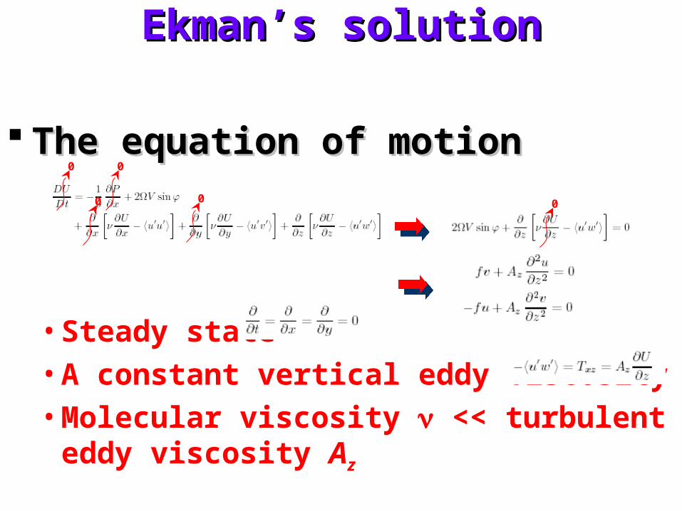
Ekman’s solutionEkman’s solution

The equation of motionThe equation of motion

• Steady state

• A constant vertical eddy viscosity

• Molecular viscosity << turbulent eddy viscosity Az

0 0

00 0

Ekman’s solutionEkman’s solution

SolutionSolution• Equation

• Solution

• The Ekman spiral (Fig 9.3)Surface velocity

Exponentially decays with depthSpiral

• Ekman’s constantsNeed two of three parameters (T, V0, Az)

Bulk formula: T = air CDU102

V0 = V0(U10, ) (Eq. 9.14)

Ekman’s solution (cont.)Ekman’s solution (cont.)

Ekman layer depthEkman layer depth• V(DE) is opposite to V0

• DE = / a (Eq. 9.15 and 9.16)

• Table 9.3: Typical Ekman Depth

The Ekman numberThe Ekman number• Ratio of the friction force and the Corilis force

• Eq. 9.17: Ez

• Eq. 9.18: at the Ekman depth DE, Ez = 1 / (22)

Bottom Ekman layerBottom Ekman layer

SolutionSolution• Eq. 9.19

u = U [1 - exp(-az)] cos azv = U exp(-az) sin az

• Boundary conditions: u(zb) = v(zb) = 0

• The Ekman spiral (Fig 9.4)Direction: anti-cyclonicAmplitude

Bottom Ekman layer (cont.)Bottom Ekman layer (cont.)

DirectionDirection• U(z = 0-) is in the direction of U(z > zb) // p

U(z > zb) p

U(z > zb) // p

U(z = 0+) is 450 to the left of U(z > zb)

U(z = 0-) is 450 to the right of U(z = 0+)Fig 9.5

Examining Ekman’s assumptionsExamining Ekman’s assumptions

No boundariesNo boundaries• Valid away from coasts

Deep waterDeep water• Valid if depth >> 200 m

ff-plane-plane• Valid

Steady stateSteady state• Valid if wind blows for longer than a pendulum day• Time-dependent solution (Hasselmann 1970)

Examining Ekman’s assumptions Examining Ekman’s assumptions (cont.)(cont.)

AAzz = = fnfn((UU101022) ) fnfn((zz))

• Not a good assumptionIf MLD < DE Az = fn(z) from MLD to DE

Homogeneous density Homogeneous density fnfn((zz))• Probably good, except as it effects stability

Observations of flow Observations of flow near the sea surfacenear the sea surface

Measurements Measurements Ekman's theory is remarkably goodEkman's theory is remarkably good• Results indicate:

Inertial currents the largest component of the flowThe flow is nearly independent of depth within the mixed layer for

periods near the inertial period. Thus the mixed layer moves like a slab at the inertial period. Current shear is concentrated at the top of the thermocline

The flow averaged over many inertial periods is almost exactly that calculated from Ekman's theory. The shear of the Ekman currents extends through the averaged mixed layer and into the thermocline. The Ekman-layer depth DE is almost exactly that proposed by Ekman (9.16), but the surface current V0 is half his value (9.14)

The transport is 900 to the right of the wind in the northern hemisphere. The transport direction agrees well with Ekman's theory

Ekman mass transportEkman mass transport

DefinitionDefinition• The integral of the UE, VE from the surface to a

depth d below the Ekman layer (Fig 9.6)

Ekman mass transport (cont.)Ekman mass transport (cont.)

Volume transportVolume transport• Definition:

The mass transport divided by the density of water and multiplied by the width perpendicular to the transport

Y: the north-south distance across which the eastward transport Qx is calculated

X: the east-west distance across which the northward transport Qy is calculated

• Unit: Sv

Application of Ekman theoryApplication of Ekman theory

Importance of upwellingImportance of upwelling• Enhance biological productivity, which feeds fisheries • Cold upwelled water alters local weather. Weather

onshore of regions of upwelling tend to have fog, low stratus clouds, a stable stratified atmosphere, little convection, and little rain.

• Spatial variability of transports in the open ocean leads to upwelling and downwelling, which leads to redistribution of mass in the ocean, which leads to wind-driven geostrophic currents via Ekman pumping

Application of Ekman theory (cont.)Application of Ekman theory (cont.)

Coastal upwellingCoastal upwelling• Along California coast north wind offshore Ekman transport (Fig 9.7 left) upwelling (Fig 9.7 right) region of cold water (Fig 10.16)

• Upwelling nutrient productivityImportant regions:

Peru, California, Somalia, Morocco, and Namibia

Application of Ekman theory (cont.)Application of Ekman theory (cont.)

Explain why the same latitude but different Explain why the same latitude but different climateclimate• region of cold water

cools the incoming air close to the sea a thin, cool atmospheric boundary layer cooling the city

• Hadley circulation in the atmosphere (Fig 4.3) downward velocity the warmer air above the boundary layer inhibits vertical convection rain is rareRain forms only when winter storms coming ashore bring strong

convection higher up in the atmosphere

Application of Ekman theory (cont.)Application of Ekman theory (cont.)

Explain why the same latitude but Explain why the same latitude but different climate (cont.)different climate (cont.)• Other reasons

MLD tends to be thin on the eastern side of oceans upwelling can easily bring up cold water

Currents along the eastern side of oceans at mid-latitudes bring colder water from higher latitudes

• All these processes are reversed offshore of east coasts

Ekman pumpingEkman pumping

Conservation of massConservation of mass• The spatial variability of the transports vertical

velocities at the top of the Ekman layer

ME: vector mass transport due to Ekman flow in the upper ocean

H: the horizontal divergence operator

0

Ekman pumping (cont.)Ekman pumping (cont.)

Relate Ekman pumping to the wind Relate Ekman pumping to the wind stressstress• The spatial variability of the transports

vertical velocities at the top of the Ekman layerSubstituteInto

T: the vector wind stress ∵ no penetration w(0) = 0 ∴ need another vertical velocity to balance

the geostrophic velocity wG(0) at the top of the interior flow in the ocean

Important conceptsImportant concepts

• Changes in wind stress produce transient oscillations in the ocean called inertial currents

Inertial currents are very common in the oceanThe period of the current is (2)/f

• Steady winds produce a thin boundary layer, the Ekman layer, at the top of the ocean

Ekman boundary layers also exist at the bottom of the ocean and the atmosphere

The Ekman layer in the atmosphere above the sea surface is called the planetary boundary layer.

• The Ekman layer at the sea surface has the following characteristics:

Direction: 450 to the right of the wind looking downwind in the Northern Hemisphere

Surface Speed: 1–2.5% of wind speed depending on latitudeDepth: approximately 40–300 m depending on latitude and wind velocity

Important concepts (cont.)Important concepts (cont.)

• Careful measurements of currents near the sea surface show that:Inertial oscillations are the largest component of the current in the

mixed layerThe flow is nearly independent of depth within the mixed layer for

periods near the inertial period. Thus the mixed layer moves like a slab at the inertial period

An Ekman layer exists in the atmosphere just above the sea (and land) surface

Surface drifters tend to drift parallel to lines of constant atmospheric pressure at the sea surface. This is consistent with Ekman’s theory.

The flow averaged over many inertial periods is almost exactly that calculated from Ekman’s theory

• Transport is 900 to the right of the wind in the northern hemisphere

Important concepts (cont)Important concepts (cont)

• Spatial variability of Ekman transport, due to spatial variability of winds over distances of hundreds of kilometers and days, leads to convergence and divergence of the transport. (a) Winds blowing toward the equator along west coasts of continents

produces upwelling along the coast. This leads to cold, productive waters within about 100 km of the shore.

(b) Upwelled water along west coasts of continents modifies the weather along the west coasts.

• Ekman pumping, which is driven by spatial variability of winds, drives a vertical current, which drives the interior geostrophic circulation of the ocean.

Momentum EquationMomentum Equation

Equation 9.1Equation 9.1

0

0

0

000

000

000

Equation 9.2Equation 9.2

0

0

0

Equation 9.4Equation 9.4

Ekman’s solutionEkman’s solution0 0

00

zA