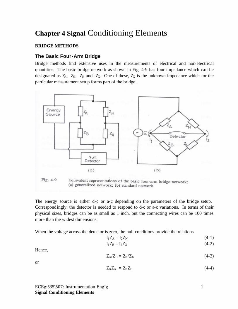
ECEg:535\507:-Instrumentation Eng’g 1 Signal Conditioning Elements

Chapter 4 Signal Conditioning Elements BRIDGE METHODS

The Basic Four-Arm Bridge Bridge methods find extensive uses in the measurements of electrical and non-electrical quantities. The basic bridge network as shown in Fig. 4-9 has four impedance which can be designated as ZA, ZB, ZN and ZX. One of these, ZX is the unknown impedance which for the particular measurement setup forms part of the bridge.

The energy source is either d-c or a-c depending on the parameters of the bridge setup. Correspondingly, the detector is needed to respond to d-c or a-c variations. In terms of their physical sizes, bridges can be as small as 1 inch, but the connecting wires can be 100 times more than the widest dimensions. When the voltage across the detector is zero, the null conditions provide the relations

I1ZA = I2ZN (4-1) I1ZB = I2ZX (4-2)

Hence, ZA/ZB = ZN/ZX (4-3)

or ZXZA = ZNZB (4-4)

ECEg:535\507:-Instrumentation Eng’g 2 Signal Conditioning Elements

This is the basic balance condition. In general, since each of the four impedance elements may be complex, then in polar form the Z's can be expressed as follows:

)8.4(

)7.4(

)6.4(

)5.4(

X

N

B

A

jXXXX

jNNNN

jBBBB

jAAAA

eZjXRZ

eZjXRZ

eZjXRZ

eZjXRZ

?

?

?

?

???

???

???

???

In Eqns. (4-5) to (4-8), the R's and the X's are thus the resistive and reactive components of the bridge arms, and the ? 's are the phasor angles. The balance condition Eqn. (4-4), must then satisfy the magnitude condition

)9.4(BNAX ZZZZ ?

From which,

? ?10.4A

BNX Z

ZZZ ?

And from the phase balance condition, ?A + ?X = ?N + ?B (4-11)

And thus yielding ?X = ?N + ?B - ?A (4-12).

Each one of the bridge arms can have fixed or adjustable values with series or shunt connected circuit parameters. Bridge circuits in which two series-connected adjustable circuits elements are located in a single arm adjacent to the unknown arm (e.g. ZB) are called ratio-arm bridges. Bridge circuits in which two shunt-connected adjustable elements both located in the arm opposite the unknown (e.g. ZA) and the product of impedance in the remaining arms is either purely real or purely imaginary are called product-arm bridges. We shall next consider some of the important types of bridges commonly used in various applications.

DC Bridges(Resistance Bridge) With a d-c galvanometer used as a detector, and with the basic bridge of Fig. 4-9 becomes a d-c bridge.

ZA = RA, ZB = RB, ZN = RN, and ZX = RX, It is the well-known Wheatstone bridge. It is almost the standard means of measuring resistance based on resistance variations over wide ranges. By means of a suitable variation of the values of RA and RB, the ratio arms, maximum sensitivities to unbalance due to RX can be detected. The ratio RN/RA should be so chosen that the unknown resistance is determined to the full number of significant figures available, which in standard Wheatstone bridges is usually four. Special difficulties can be encountered in the measurement of very low and very high resistance or resistance variations. With low resistance, using what is known as the Kelvin double bridge (Fig. 4-10) which is a modification of the Whetstone Bridge can reduce the uncertainty introduced by the resistance of leads and contacts.

ECEg:535\507:-Instrumentation Eng’g 3 Signal Conditioning Elements

With iD = 0, the balance condition becomes

)13.4(qp

QP

rqpqr

QPS

X ???

??

Where r is the resistance of connection between RB = S and RX = X. By taking P = p and q = Q, and with r assumed to be very small, Eqn. (4-13) becomes

)14.4(A

BN

RRR

QPS

X ??

Variations in the unknown resistance, and the effects of contact and lead resistance are greatly minimized. Still, the effects of what are known as thermoelectric emfs can be easily eliminated. By reversing currents through RB = S and RX = X, and by averaging the values detected for X, more accurate values for X can be obtained. Values of resistance which can be measured by the Kelvin bridge may range from 1000? to 0.100m? with error estimates ranging from 0.1 to 0.01 percent. When the resistance being measured is very high, the bridge galvanometer becomes a relatively insensitive indicator of unbalanced conditions. This is because of the high source impedance that the bridge presents to the galvanometer. The difficulty can be overcome by using a d-c vacuum tube voltmeter (VTVM), a digital voltmeter (DVM), or a cathode ray oscilloscope (CRO) in place of the galvanometer. Also, in practice it is better to use a fixed value RN = 1M? and to balance the bridge by varying RB.

ECEg:535\507:-Instrumentation Eng’g 4 Signal Conditioning Elements

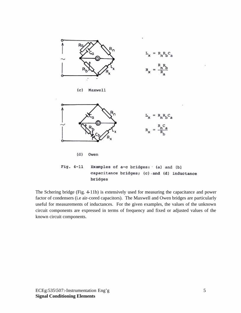
AC Bridges Detectors commonly used in d-c bridges are vibration galvanometers (with sensitivities of 50Hz to 1 KHz), earphones (from about 250Hz), and tunable amplifier detectors (from about 10Hz to 100 KHz). For wider bandwidths, CROs with relatively high sensitivities could also be used. The possible variations of the bridge arms are described in Eqs. (4-9) and (4-11). Based on these balance conditions various a-c bridges are used in practice under the broad Classification of capacitance and inductance bridges. Some examples are shown in Fig. 4-11. The Wien bridge (Fig. 4-11a) finds use in the measurement of frequency in the audio ranges. It is also useful in the precision determination of capacitance, since the standards of frequency and resistance is known to a very great accuracy.

ECEg:535\507:-Instrumentation Eng’g 5 Signal Conditioning Elements

The Schering bridge (Fig. 4-11b) is extensively used for measuring the capacitance and power factor of condensers (i.e air-cored capacitors). The Maxwell and Owen bridges are particularly useful for measurements of inductances. For the given examples, the values of the unknown circuit components are expressed in terms of frequency and fixed or adjusted values of the known circuit components.

ECEg:535\507:-Instrumentation Eng’g 6 Signal Conditioning Elements

Examples of Signal Conditioning Elements (Note the strain gauges replaced by any passive sensors) Strain gauges using bridge measurement circuit

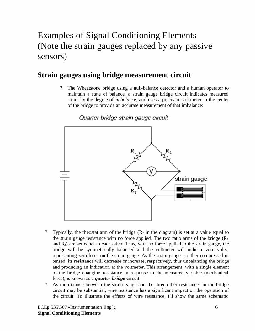
? The Wheatstone bridge using a null-balance detector and a human operator to maintain a state of balance, a strain gauge bridge circuit indicates measured strain by the degree of imbalance, and uses a precision voltmeter in the center of the bridge to provide an accurate measurement of that imbalance:

? Typically, the rheostat arm of the bridge (R2 in the diagram) is set at a value equal to the strain gauge resistance with no force applied. The two ratio arms of the bridge (R1 and R3) are set equal to each other. Thus, with no force applied to the strain gauge, the bridge will be symmetrically balanced and the voltmeter will indicate zero volts, representing zero force on the strain gauge. As the strain gauge is either compressed or tensed, its resistance will decrease or increase, respectively, thus unbalancing the bridge and producing an indication at the voltmeter. This arrangement, with a single element of the bridge changing resistance in response to the measured variable (mechanical force), is known as a quarter-bridge circuit.

? As the distance between the strain gauge and the three other resistances in the bridge circuit may be substantial, wire resistance has a significant impact on the operation of the circuit. To illustrate the effects of wire resistance, I'll show the same schematic

ECEg:535\507:-Instrumentation Eng’g 7 Signal Conditioning Elements

diagram, but add two resistor symbols in series with the strain gauge to represent the wires:

? The strain gauge's resistance (Rgauge) is not the only resistance being measured, the wire resistances Rwire1 and Rwire2, being in series with Rgauge, also contribute to the resistance of the lower half of the rheostat arm of the bridge, and consequently contribute to the voltmeter's indication. This, of course, will be falsely interpreted by the meter as physical strain on the gauge.

? While this effect cannot be completely eliminated in this configuration, it can be minimized with the addition of a third wire, connecting the right side of the voltmeter directly to the upper wire of the strain gauge:

? Because the third wire carries practically no current (due to the voltmeter's extremely high internal resistance), its resistance will not drop any substantial amount of voltage.

ECEg:535\507:-Instrumentation Eng’g 8 Signal Conditioning Elements

Notice how the resistance of the top wire (Rwire1) has been "bypassed" now that the voltmeter connects directly to the top terminal of the strain gauge, leaving only the lower wire's resistance (Rwire2) to contribute any stray resistance in series with the gauge. Not a perfect solution, of course, but twice as good as the last circuit.

? There is a way, however, to reduce wire resistance error far beyond the method just described, and also help mitigate another kind of measurement error due to temperature. An unfortunate characteristic of strain gauges is that of resistance change with changes in temperature. This is a property common to all conductors, some more than others. Thus, our quarter-bridge circuit as shown (either with two or with three wires connecting the gauge to the bridge) works as a thermometer just as well as it does a strain indicator. If all we want to do is measure strain, this is not good. We can transcend this problem, however, by us ing a "dummy" strain gauge in place of R2, so that both elements of the rheostat arm will change resistance in the same proportion when temperature changes, thus canceling the effects of temperature change:

? Resistors R1 and R3 are of equal resistance value, and the strain gauges are identical to one another. With no applied force, the bridge should be in a perfectly balanced condition and the voltmeter should register 0 volts. Both gauges are bonded to the same test specimen, but only one is placed in a position and orientation so as to be exposed to physical strain (the active gauge). The other gauge is isolated from all mechanical stress, and acts merely as a temperature compensation device (the "dummy" gauge). If the temperature changes, both gauge resistances will change by the same percentage, and the bridge's state of balance will remain unaffected. Only a differential resistance (difference of resistance between the two strain gauges) produced by physical force on the test specimen can alter the balance of the bridge.

? Wire resistance doesn't impact the accuracy of the circuit as much as before, because the wires connecting both strain gauges to the bridge are approximately equal length. Therefore, the upper and lower sections of the bridge's rheostat arm contain approximately the same amount of stray resistance, and their effects tend to cancel:

ECEg:535\507:-Instrumentation Eng’g 9 Signal Conditioning Elements

? Even though there are now two strain gauges in the bridge circuit, only one is responsive to mechanical strain, and thus we would still refer to this arrangement as a quarter-bridge. However, if we were to take the upper strain gauge and position it so that it is exposed to the opposite force as the lower gauge (i.e. when the upper gauge is compressed, the lower gauge will be stretched, and vice versa), we will have both gauges responding to strain, and the bridge will be more responsive to applied force. This utilization is known as a half-bridge. Since both strain gauges will either increase or decrease resistance by the same proportion in response to changes in temperature, the effects of temperature change remain canceled and the circuit will suffer minimal temperature- induced measurement error:

ECEg:535\507:-Instrumentation Eng’g 10 Signal Conditioning Elements

? In applications where such complementary pairs of strain gauges can be bonded to the test specimen, it may be advantageous to make all four elements of the bridge "active" for even greater sensitivity. This is called a full-bridge circuit:

? Both half-bridge and full-bridge configurations grant greater sensitivity over the quarter-bridge circuit, but often it is not possible to bond complementary pairs of strain gauges to the test specimen. Thus, the quarter-bridge circuit is frequently used in strain measurement systems.

? When possible, the full-bridge configuration is the best to use. This is true not only because it is more sensitive than the others, but because it is linear while the others are not. Quarter-bridge and half-bridge circuits provide an output (imbalance) signal that is only approximately proportional to applied strain gauge force. Linearity, or proportionality, of these bridge circuits is best when the amount of resistance change due to applied force is very small compared to the nominal resistance of the gauge(s). With a full-bridge, however, the output voltage is directly proportional to applied force, with no approximation (provided that the change in resistance caused by the applied force is equal for all four strain gauges).

? Unlike the Wheatstone and Kelvin bridges, which provide measurement at a condition of perfect balance and therefore function irrespective of source voltage, the amount of source (or "excitation") voltage matters in an unbalanced bridge like this. Therefore, strain gauge bridges are rated in millivolts of imbalance produced per volt of excitation, per unit measure of force. A typical example for a strain gauge of the type used for measuring force in industrial environments is 15 mV/V at 1000 pounds. That is, at exactly 1000 pounds applied force (either compressive or tensile), the bridge will be unbalanced by 15 millivolts for every volt of excitation voltage. Again, such a figure is precise if the bridge circuit is full-active (four active strain gauges, one in each arm of the bridge), but only approximate for half-bridge and quarter-bridge arrangements.

? Strain gauges may be purchased as complete units, with both strain gauge elements and bridge resistors in one housing, sealed and encapsulated for protection from the elements, and equipped with mechanical fastening points for attachment to a machine or structure. Such a package is typically called a load cell

ECEg:535\507:-Instrumentation Eng’g 11 Signal Conditioning Elements

? In applications where such complementary pairs of strain gauges can be bonded to the test specimen, it may be advantageous to make all four elements of the bridge "active" for even greater sensitivity. This is called a full-bridge circuit:

? Both half-bridge and full-bridge configurations grant greater sensitivity over the quarter-bridge circuit, but often it is not possible to bond complementary pairs of strain gauges to the test specimen. Thus, the quarter-bridge circuit is frequently used in strain measurement systems.

ECEg:535\507:-Instrumentation Eng’g 12 Signal Conditioning Elements

OPERATIONAL AMPLIFIERS Operational amplifiers (OPAMPs) are essential components of both practical and precision analog instruments. Their uses as comparators will also be seen in comparison of measurements.. The basic characteristics of an OPAMP are: (a) high input impedance; (b) low output impedance, (c) relatively low noise, (d) relatively wide bandwidth, and (e) low drift.

As shown in Fig. 3-27(a) for most applications, an OPAMP has two inputs and one output, all referred to a ground level. Input terminals 1 and 2 are referred to as the inverting and non-inverting inputs. Because the input impedance Zin is very high, the input current Ii is negligible. The output impedance Zo is however very low, and the output voltage is hence given by

Vo = AVi - ZoIo (4-15) ? AVi (4-16) = -A(V1-V2) (4-17)

Where the amplifier gains A is assumed to be very large. With the non- inverting input grounded, and the inverting input and output terminals bridged by a feedback impedance Zf, it can be shown that

)19.4(

)(1

)(

)18.4()(

if

i

iff

ifi

i

i

O

ZZAZ

ZZAZ

ZZAZAZ

VV

??

???

???

Where Zi is the impedance on the input side as shown in Fig. 3.28. Eqn. (4-18) is the result of the application of Kirchhoff's voltage and current equations in which the input current Ii is set equal to the negative of the feedback current If. With the amplifier gain sufficiently large so that AZi/(Zi + Zf) >> 1 then

)20.4(0

i

f

i Z

Z

VV

??

ECEg:535\507:-Instrumentation Eng’g 13 Signal Conditioning Elements

The analysis leading to Eq. (4-20) is known as the virtual ground method in that the potential at V2 at the non-inverting input of the amplifier as connected in Fig. 3-27 is essentially at ground potential. The ideal characteristics of OPAMPs are limited by input offset voltage (Vs), and input bias current (Ib). The offset voltage is also referred to as the drift of voltage referred to the input. It is a measure of the imbalance in the input terminals of an OPAMP and should be zero in an ideal amplifier. The input bias current is the d-c current required at the input terminal to provide zero output voltage with no input signal or offset voltage. Both input offset voltage and input bias current drift from their normal values as functions of temperature, power supply voltage, or time.

Applications of OPAMPs in instrumentation systems range from their uses as amplifiers of weak signals to wave shaping devices. A differential amplifier can be built by applying signals V1 and V2 (Fig. 3-26a). The output voltage will be given by

Vo = A(V1-V2)+ AcVc (4-21)

Where Vc = (V1-V2)/2 is referred to as the common mode component and Ac is the common mode gain. The common mode rejection ratio is defined by

)24.4(log20)(

)23.4(

)22.4(mod

lg

CMRRdBCMRRorAA

gaineCommonainaDifferenti

CMRR

C

?

?

?

Which is required to be as low as possible. A non-inverting amplifier provides an output, which is in phase with the input (Fig. 3-28). The gain of the amplifier will be

ECEg:535\507:-Instrumentation Eng’g 14 Signal Conditioning Elements

01

)26.4(11

)25.4())(

21

12

2

1

2

12

20

?????

??

??

?

RandRifRR

ARif

RR

ARRRRA

VV i

i

??

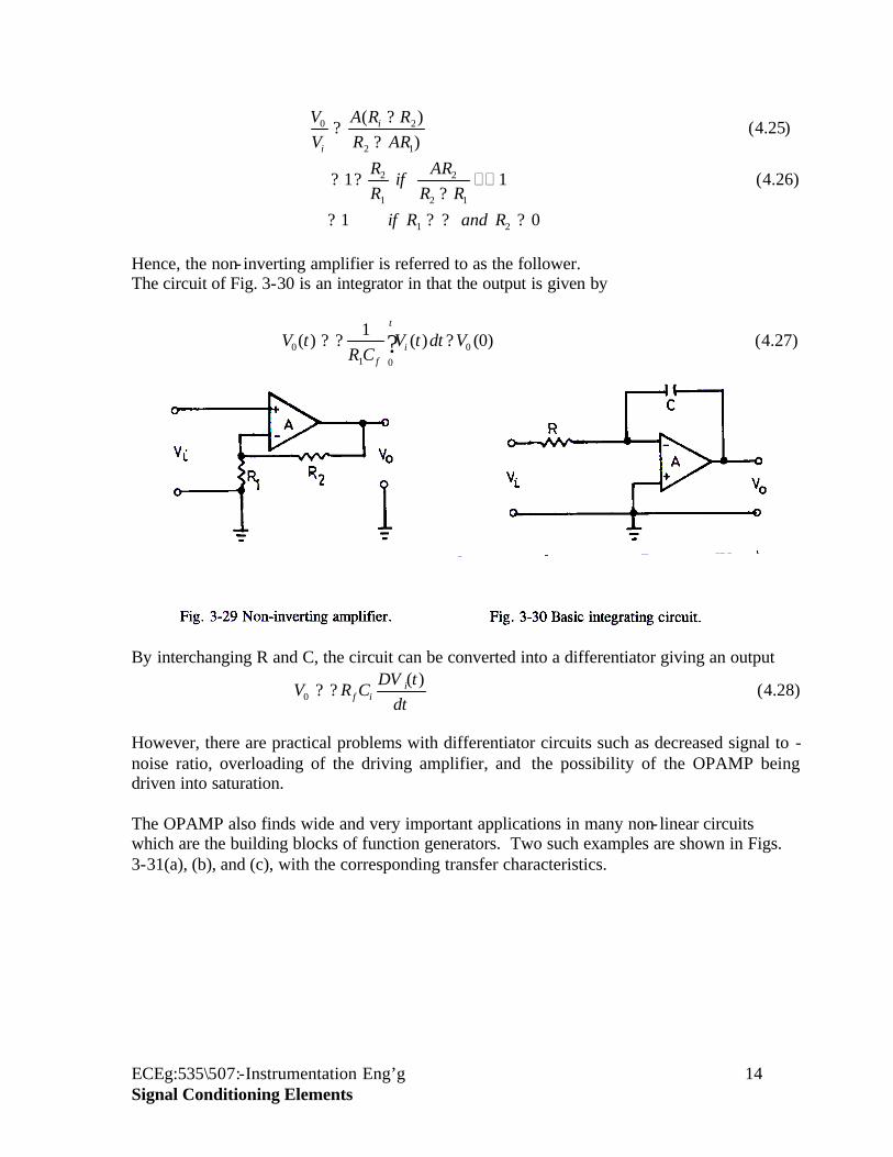
Hence, the non- inverting amplifier is referred to as the follower. The circuit of Fig. 3-30 is an integrator in that the output is given by

)27.4()0()(1

)( 001

0 VdttVCR

tVt

if

??? ?

By interchanging R and C, the circuit can be converted into a differentiator giving an output

)28.4()(

0 dttDV

CRV iif??

However, there are practical problems with differentiator circuits such as decreased signal to -noise ratio, overloading of the driving amplifier, and the possibility of the OPAMP being driven into saturation. The OPAMP also finds wide and very important applications in many non- linear circuits which are the building blocks of function generators. Two such examples are shown in Figs. 3-31(a), (b), and (c), with the corresponding transfer characteristics.

ECEg:535\507:-Instrumentation Eng’g 15 Signal Conditioning Elements