66

CHAPTER 4

SENSORLESS SPEED CONTROL OF PMBLDC MOTOR

4.1 PRINCIPLE OF CONTROL LAWS

The control objective is to bring the speed of the PMBLDC motor

to desired value by varying the voltage input, when there is variation in speed

due to servo operation (set point change) as well as regulatory operation

(disturbance rejection. (Dixon and Leal 2002) reported that precise

determination of the rotor angle is not necessary to control the speed of

PMBLDC motor. Only the position of commutation points is required to

achieve quasi-square current, with dead time periods of 60º. Hence, in the

proposed sensorless speed control of PMBLDC motor, the position of the

rotor is evaluated by measuring the phase currents.

The inverter supplies a quasi-square current, whose magnitude

IMAX

, is proportional to the machine shaft torque. Thus, by controlling the

phase currents, the torque and speed are adjusted. There are two ways to

control the phase currents of a PMBLDC motor. Accordingly, the two control

laws used in the present work are shown in Figure 4.1

67

Figure 4.1 Schematic Diagram of Control laws

In both the control laws, absolute values of the two of the three

phase currents are rectified and the dc component corresponding to the

amplitude IMAX

of the original phase current is obtained. The circuit used to

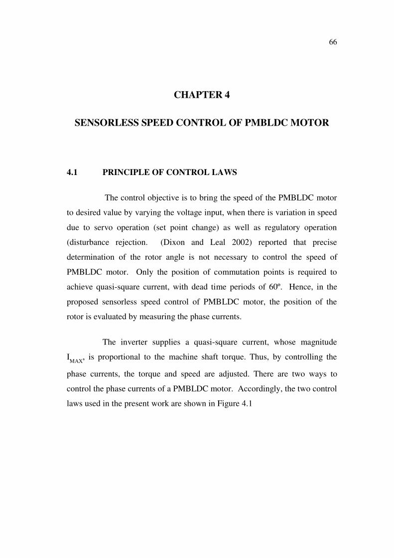
find IMAX from the original phase current is shown in Figure 4.2. The dc

component corresponding to the amplitude IMAX is compared with a reference

current IREF. The error signal thus obtained is processed through a controller.

R= 1K C = 1000 µF D1- D4= IN4007

Ron = 0.001 K1= 0.001

Figure 4.2 Simulation circuit to find the amplitude IMAX

68

4.2 DESIGN OF PI CONTROLLER

The DC input voltage is applied to the three phase inverter as in

Figure 4.3. The gate signal for the inverter is obtained by sensing the position

of the rotor. The simulation is carried out to study the variation of speed for

the variation in DC input voltage.

4.2.1 Open loop response of VSI fed PMBLDC Motor

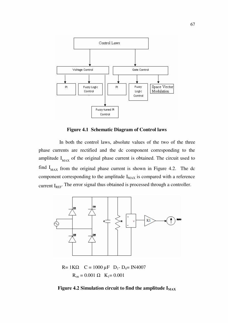
Figure 4.3 shows the simulation circuit used for carrying out open

loop studies of VSI fed PMBLDC motor. The input is the DC voltage in volts

and the output is speed in rpm.

Figure 4.3 Open loop simulation circuit of VSI fed PMBLDC motor

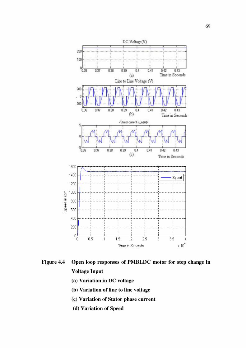
Figure 4.4 shows the open loop speed response of the VSI fed

PMBLDC motor. Figure 4.4(a) shows the DC voltage applied to the three

phase inverter. Figure 4.4(b) shows the line to line voltage applied to the

stator coil of PMBLDC motor. Figure 4.4(c) gives the response of stator

phase current. Figure 4.4(d) shows the speed response. It is clearly seen in

Speed curve that there is an overshoot and it resembles the second order

response.

69

Figure 4.4 Open loop responses of PMBLDC motor for step change in

Voltage Input

(a) Variation in DC voltage

(b) Variation of line to line voltage

(c) Variation of Stator phase current

(d) Variation of Speed

70

(4.2)

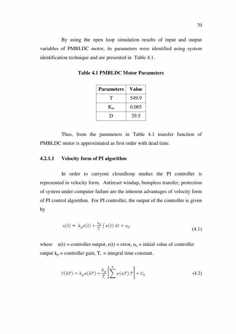
By using the open loop simulation results of input and output

variables of PMBLDC motor, its parameters were identified using system

identification technique and are presented in Table 4.1.

Table 4.1 PMBLDC Motor Parameters

Parameters Value

T 549.9

Km 6.065

D 29.5

Thus, from the parameters in Table 4.1 transfer function of

PMBLDC motor is approximated as first order with dead time.

4.2.1.1 Velocity form of PI algorithm

In order to carryout closedloop studies the PI controller is

represented in velocity form. Antireset windup, bumpless transfer, protection

of system under computer failure are the inherent advantages of velocity form

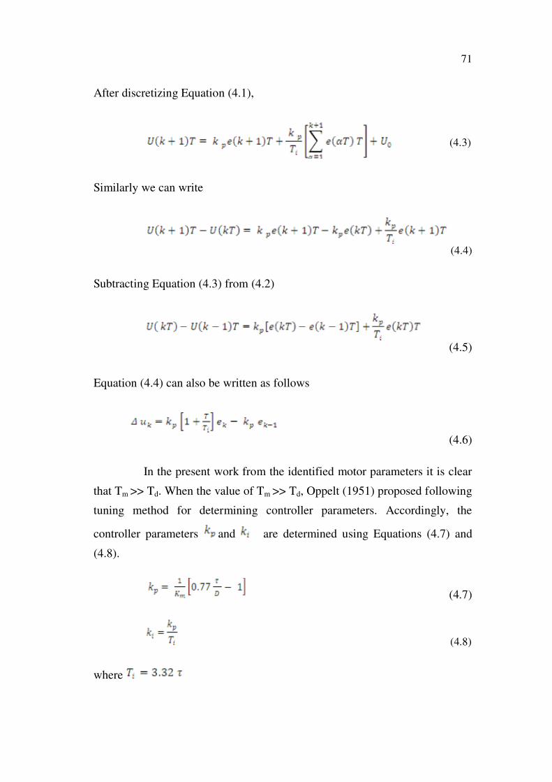
of PI control algorithm. For PI controller, the output of the controller is given

by

(4.1)

where u(t) = controller output, e(t) = error, uo = initial value of controller

output kp = controller gain, Ti = integral time constant.

71

(4.3)

After discretizing Equation (4.1),

Similarly we can write

(4.4)

Subtracting Equation (4.3) from (4.2)

(4.5)

Equation (4.4) can also be written as follows

(4.6)

In the present work from the identified motor parameters it is clear

that Tm >> Td. When the value of Tm >> Td, Oppelt (1951) proposed following

tuning method for determining controller parameters. Accordingly, the

controller parameters and are determined using Equations (4.7) and

(4.8).

(4.7)

(4.8)

where

72

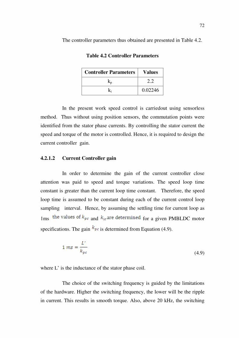
The controller parameters thus obtained are presented in Table 4.2.

Table 4.2 Controller Parameters

Controller Parameters Values

kp 2.2

ki 0.02246

In the present work speed control is carriedout using sensorless

method. Thus without using position sensors, the commutation points were

identified from the stator phase currents. By controlling the stator current the

speed and torque of the motor is controlled. Hence, it is required to design the

current controller gain.

4.2.1.2 Current Controller gain

In order to determine the gain of the current controller close

attention was paid to speed and torque variations. The speed loop time

constant is greater than the current loop time constant. Therefore, the speed

loop time is assumed to be constant during each of the current control loop

sampling interval. Hence, by assuming the settling time for current loop as

1ms and for a given PMBLDC motor

specifications. The gain is determined from Equation (4.9).

(4.9)

where L’ is the inductance of the stator phase coil.

The choice of the switching frequency is guided by the limitations

of the hardware. Higher the switching frequency, the lower will be the ripple

in current. This results in smooth torque. Also, above 20 kHz, the switching

73

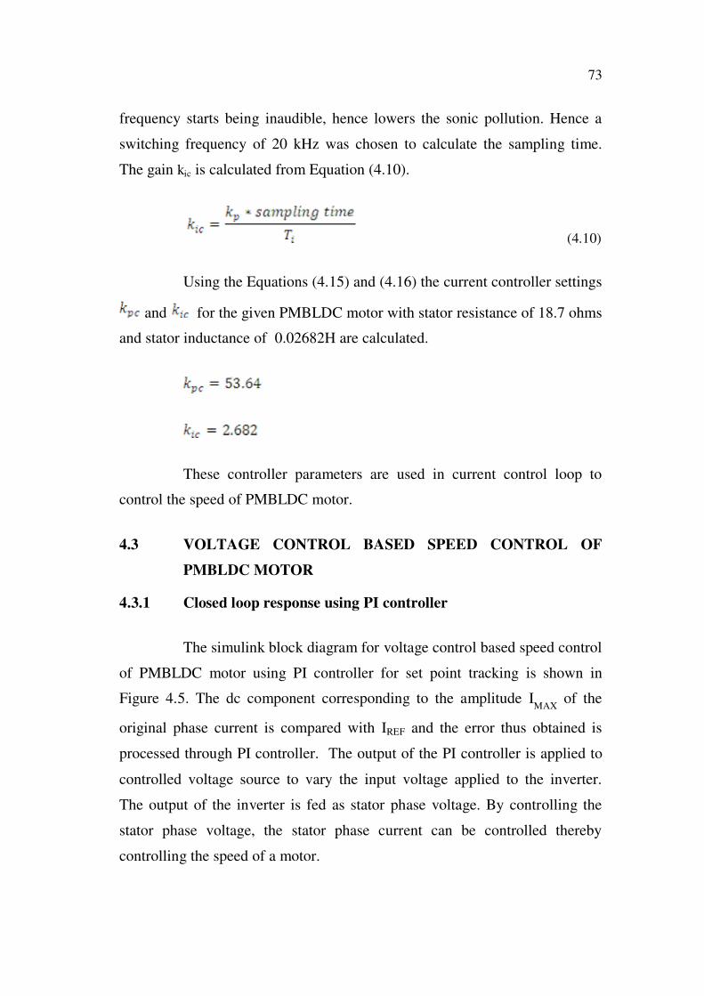
frequency starts being inaudible, hence lowers the sonic pollution. Hence a

switching frequency of 20 kHz was chosen to calculate the sampling time.

The gain kic is calculated from Equation (4.10).

(4.10)

Using the Equations (4.15) and (4.16) the current controller settings

and for the given PMBLDC motor with stator resistance of 18.7 ohms

and stator inductance of 0.02682H are calculated.

These controller parameters are used in current control loop to

control the speed of PMBLDC motor.

4.3 VOLTAGE CONTROL BASED SPEED CONTROL OF

PMBLDC MOTOR

4.3.1 Closed loop response using PI controller

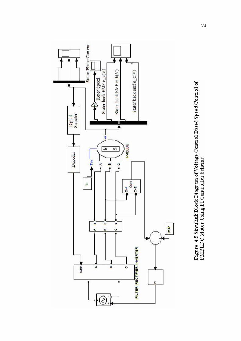
The simulink block diagram for voltage control based speed control

of PMBLDC motor using PI controller for set point tracking is shown in

Figure 4.5. The dc component corresponding to the amplitude IMAX

of the

original phase current is compared with IREF and the error thus obtained is

processed through PI controller. The output of the PI controller is applied to

controlled voltage source to vary the input voltage applied to the inverter.

The output of the inverter is fed as stator phase voltage. By controlling the

stator phase voltage, the stator phase current can be controlled thereby

controlling the speed of a motor.

74

75

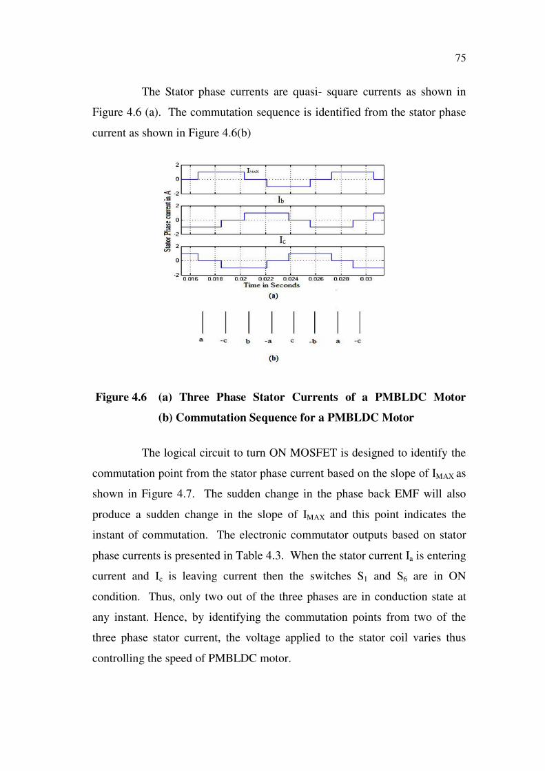
The Stator phase currents are quasi- square currents as shown in

Figure 4.6 (a). The commutation sequence is identified from the stator phase

current as shown in Figure 4.6(b)

Figure 4.6 (a) Three Phase Stator Currents of a PMBLDC Motor

(b) Commutation Sequence for a PMBLDC Motor

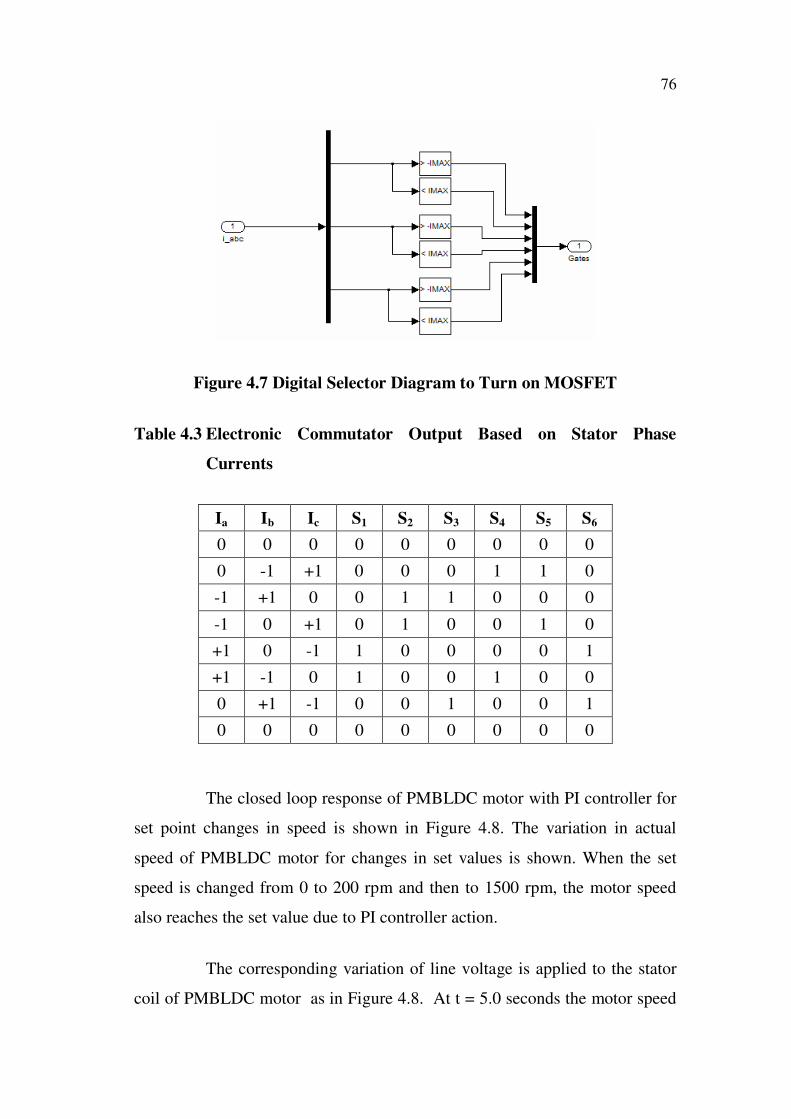
The logical circuit to turn ON MOSFET is designed to identify the

commutation point from the stator phase current based on the slope of IMAX as

shown in Figure 4.7. The sudden change in the phase back EMF will also

produce a sudden change in the slope of IMAX and this point indicates the

instant of commutation. The electronic commutator outputs based on stator

phase currents is presented in Table 4.3. When the stator current Ia is entering

current and Ic is leaving current then the switches S1 and S6 are in ON

condition. Thus, only two out of the three phases are in conduction state at

any instant. Hence, by identifying the commutation points from two of the

three phase stator current, the voltage applied to the stator coil varies thus

controlling the speed of PMBLDC motor.

76

Figure 4.7 Digital Selector Diagram to Turn on MOSFET

Table 4.3 Electronic Commutator Output Based on Stator Phase

Currents

Ia Ib Ic S1 S2 S3 S4 S5 S6

0 0 0 0 0 0 0 0 0

0 -1 +1 0 0 0 1 1 0

-1 +1 0 0 1 1 0 0 0

-1 0 +1 0 1 0 0 1 0

+1 0 -1 1 0 0 0 0 1

+1 -1 0 1 0 0 1 0 0

0 +1 -1 0 0 1 0 0 1

0 0 0 0 0 0 0 0 0

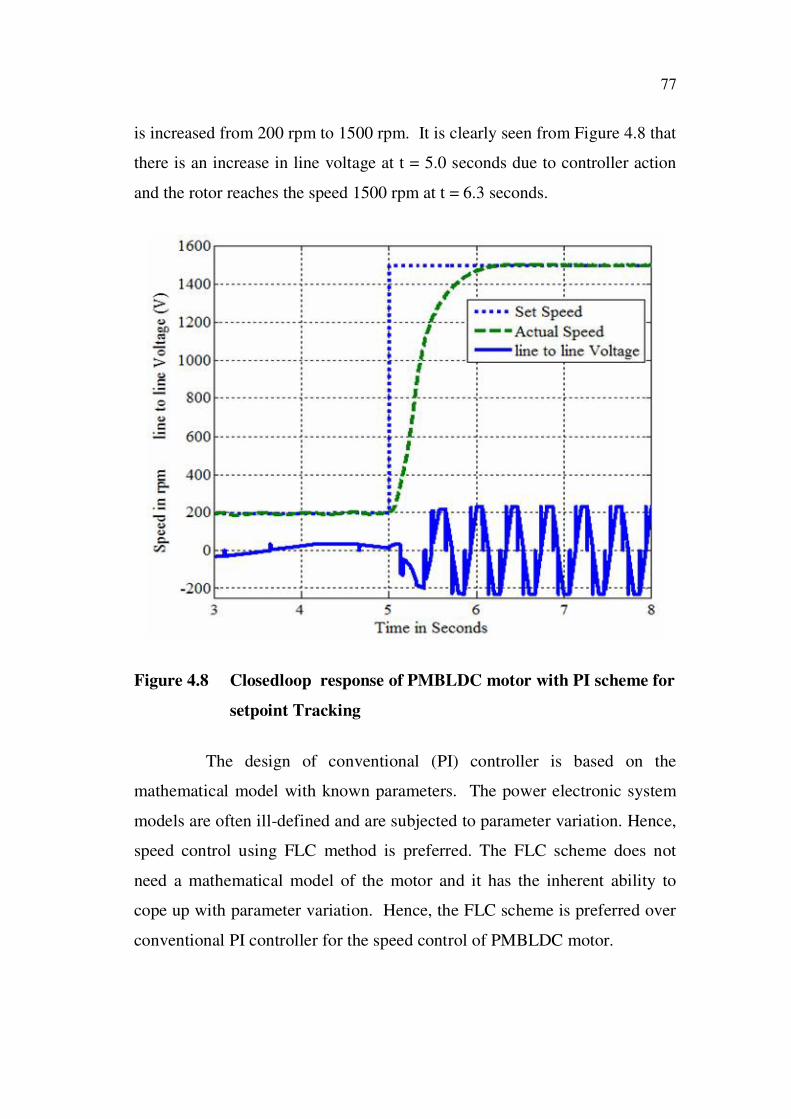
The closed loop response of PMBLDC motor with PI controller for

set point changes in speed is shown in Figure 4.8. The variation in actual

speed of PMBLDC motor for changes in set values is shown. When the set

speed is changed from 0 to 200 rpm and then to 1500 rpm, the motor speed

also reaches the set value due to PI controller action.

The corresponding variation of line voltage is applied to the stator

coil of PMBLDC motor as in Figure 4.8. At t = 5.0 seconds the motor speed

77

is increased from 200 rpm to 1500 rpm. It is clearly seen from Figure 4.8 that

there is an increase in line voltage at t = 5.0 seconds due to controller action

and the rotor reaches the speed 1500 rpm at t = 6.3 seconds.

Figure 4.8 Closedloop response of PMBLDC motor with PI scheme for

setpoint Tracking

The design of conventional (PI) controller is based on the

mathematical model with known parameters. The power electronic system

models are often ill-defined and are subjected to parameter variation. Hence,

speed control using FLC method is preferred. The FLC scheme does not

need a mathematical model of the motor and it has the inherent ability to

cope up with parameter variation. Hence, the FLC scheme is preferred over

conventional PI controller for the speed control of PMBLDC motor.

78

4.3.2 Voltage Control Method using FLC Scheme

4.3.2.1 Fuzzy Logic Controller Design

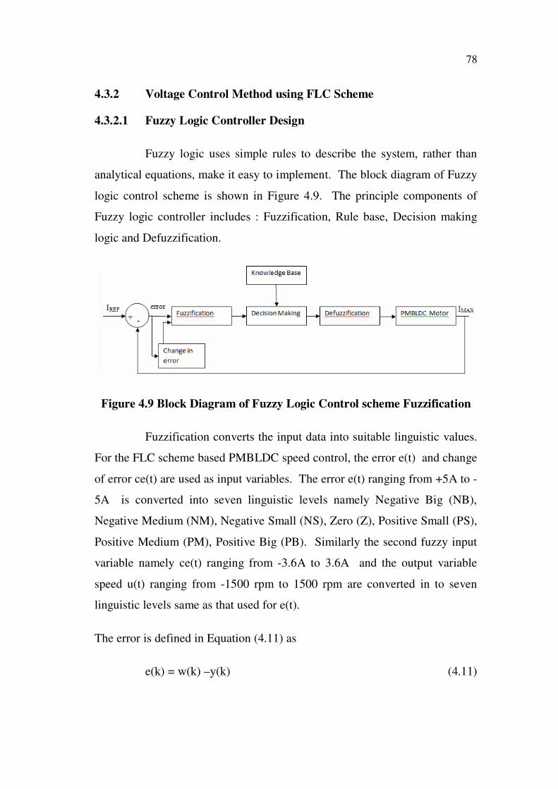
Fuzzy logic uses simple rules to describe the system, rather than

analytical equations, make it easy to implement. The block diagram of Fuzzy

logic control scheme is shown in Figure 4.9. The principle components of

Fuzzy logic controller includes : Fuzzification, Rule base, Decision making

logic and Defuzzification.

Figure 4.9 Block Diagram of Fuzzy Logic Control scheme Fuzzification

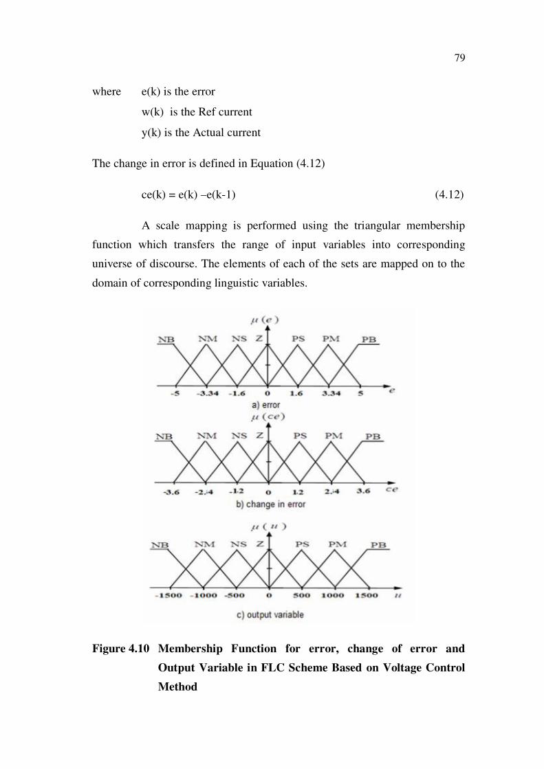
Fuzzification converts the input data into suitable linguistic values.

For the FLC scheme based PMBLDC speed control, the error e(t) and change

of error ce(t) are used as input variables. The error e(t) ranging from +5A to -

5A is converted into seven linguistic levels namely Negative Big (NB),

Negative Medium (NM), Negative Small (NS), Zero (Z), Positive Small (PS),

Positive Medium (PM), Positive Big (PB). Similarly the second fuzzy input

variable namely ce(t) ranging from -3.6A to 3.6A and the output variable

speed u(t) ranging from -1500 rpm to 1500 rpm are converted in to seven

linguistic levels same as that used for e(t).

The error is defined in Equation (4.11) as

e(k) = w(k) –y(k) (4.11)

79

where e(k) is the error

w(k) is the Ref current

y(k) is the Actual current

The change in error is defined in Equation (4.12)

ce(k) = e(k) –e(k-1) (4.12)

A scale mapping is performed using the triangular membership

function which transfers the range of input variables into corresponding

universe of discourse. The elements of each of the sets are mapped on to the

domain of corresponding linguistic variables.

Figure 4.10 Membership Function for error, change of error and

Output Variable in FLC Scheme Based on Voltage Control

Method

80

Care is taken to ensure that the cross point level for every membership

function with degree of membership, is greater than zero. This means that

every crisp value belongs to atleast one membership value greater than zero.

If this is not the case, no rule will fire and there will not be any control

action. The membership function for input variables and output variable are

shown in Figure 4.10.

Rule Base

The rule base is constructed using expert knowledge and

experience. The rules are expressed in the form of following syntax:

IF < Fuzzy Preposition > THEN < Fuzzy Preposition >.

‘IF’ part is called antecedent. ‘THEN’ part is called consequent. In

the present work e(t), ce(t) are antecedents and control command is the

consequent. The combination is called the premise. The rules are generated

heuristically from the response of the conventional controller. In the present

work, 49 rules are derived from the analysis of trend obtained from the

simulation results obtained from the PI controller scheme and are presented in

Table 4.4 and 4.5.

If both error and change in error are zero, then maintain the present

control setting. If error is not zero but the output is approaching the

satisfactory rate, then maintain the present control setting. If error is growing,

then change the control signal depending on the magnitude and sign of error

and change in error, to force error towards zero.

81

Table 4.4 Rule Base Matrix for Voltage Control Based Speed Control

of PMBLDC Motor Using FLC Scheme

e(k)/ ce(k) NB NM NS Z PS PM PB

NB NB NB NB NB NM NS Z

NM NB NB NB NM NS Z PS

NS NB NB NM NS Z PS PM

Z NB NM NS Z PS PM PB

PS NM NS Z PS PM PB PB

PM NS Z PS PM PB PB PB

PB Z PS PM PB PB PB PB

NB (Negative Big), NM (Negative Medium), NS (negative Small), Z (Zero),

PS (Positive Small), PM (Positive Medium), PB (positive Big).

The inference of Rule Base Matrix is given in Table 4.5

Table 4.5 Inference of Rule Base Matrix

Zone Rule Interpretation

e(k) 0and ce (k) 0 implies set point output. Therefore

error is not self correcting. The magnitude of controller

output changes based on the magnitude of e(k) and ce(k).

e(k) < 0and ce (k) > 0 implies set point < output. Therefore

error is self correcting and change in output is almost zero,

that is control variable remains at its present setting.

e(k) > 0 and ce (k) < 0 implies set point > output. Therefore

error is self-correcting and change in output is almost zero

that is control variable remains at its present setting.

e(k) 0 and ce(k) 0 implies set point output. Therefore

error is not self correcting. The magnitude of controller

output changes based on the magnitude of e(k) and ce(k).

Both e(k) and ce(k) is closer to zero. The system is in steady

state. The change in controller output is zero. That is the

present control setting is maintained.

82

Decision making logic

The decision making logic, infers a system of rules through fuzzy

operators namely ‘AND’ and ‘OR’ for finding ‘minimum’ and ‘maximum’

values respectively. In other words, ‘Max-Min’ criterion is used to combine

the results to generate single truth value, which determines the outcome of the

rules. Thus, the outcome of the decision making logic is the inferred fuzzy

control action. In the present work, the single truth value is obtained using

Max-Min criteria.

Defuzzification

The output of the rule base is converted into crisp value, using

defuzzification module. The commonly used defuzzification methods are i)

Max criteria ii) Mean of maximum iii) Center of Area method. The

Defuzzification using Center of Area is considered for this application as it

produces the results which are sensitive to all the rules and the output moves

smoothly across the control surface which can reduce the wear and tear of

final control element. The Table 4.6 shows the FLC design parameters for the

voltage control based speed control of PMBLDC motor. The crisp output

(4.13)

2(Wj) = Maximum value of the membership function corresponding

to jth

quantisation level.

where j = 1 to n is the number of quantisation levels

Wj = support value at which the membership function reaches

maximum value.

83

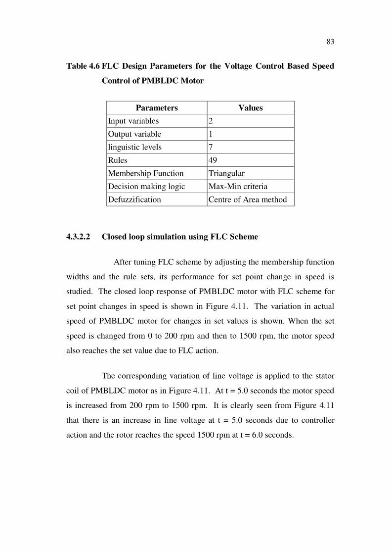
Table 4.6 FLC Design Parameters for the Voltage Control Based Speed

Control of PMBLDC Motor

Parameters Values

Input variables 2

Output variable 1

linguistic levels 7

Rules 49

Membership Function Triangular

Decision making logic Max-Min criteria

Defuzzification Centre of Area method

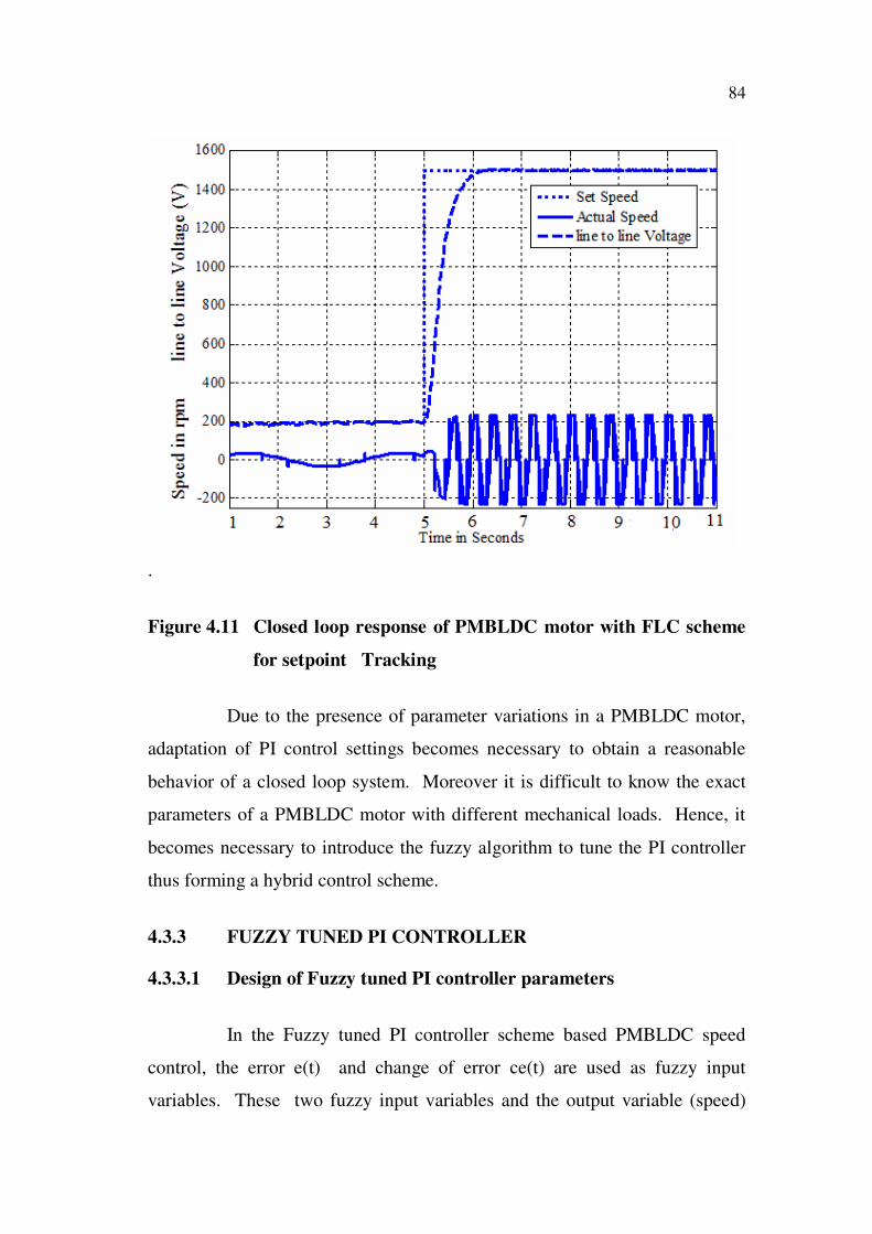
4.3.2.2 Closed loop simulation using FLC Scheme

After tuning FLC scheme by adjusting the membership function

widths and the rule sets, its performance for set point change in speed is

studied. The closed loop response of PMBLDC motor with FLC scheme for

set point changes in speed is shown in Figure 4.11. The variation in actual

speed of PMBLDC motor for changes in set values is shown. When the set

speed is changed from 0 to 200 rpm and then to 1500 rpm, the motor speed

also reaches the set value due to FLC action.

The corresponding variation of line voltage is applied to the stator

coil of PMBLDC motor as in Figure 4.11. At t = 5.0 seconds the motor speed

is increased from 200 rpm to 1500 rpm. It is clearly seen from Figure 4.11

that there is an increase in line voltage at t = 5.0 seconds due to controller

action and the rotor reaches the speed 1500 rpm at t = 6.0 seconds.

84

.

Figure 4.11 Closed loop response of PMBLDC motor with FLC scheme

for setpoint Tracking

Due to the presence of parameter variations in a PMBLDC motor,

adaptation of PI control settings becomes necessary to obtain a reasonable

behavior of a closed loop system. Moreover it is difficult to know the exact

parameters of a PMBLDC motor with different mechanical loads. Hence, it

becomes necessary to introduce the fuzzy algorithm to tune the PI controller

thus forming a hybrid control scheme.

4.3.3 FUZZY TUNED PI CONTROLLER

4.3.3.1 Design of Fuzzy tuned PI controller parameters

In the Fuzzy tuned PI controller scheme based PMBLDC speed

control, the error e(t) and change of error ce(t) are used as fuzzy input

variables. These two fuzzy input variables and the output variable (speed)

85

are converted into seven linguistic levels namely Negative Big (NB),

Negative Medium (NM), Negative Small(NS), Zero(Z), Positive Small(PS),

Positive Medium(PM), Positive Big(PB). The symmetrical triangular

membership function transfers the range of input variables into corresponding

universe of discourse. The rule base is constructed using expert knowledge.

The outcome of the decision making logic infers the fuzzy control action. The

single truth value is obtained using Max-Min criteria. The defuzzified (crisp)

value is obtained using Center of Area method .

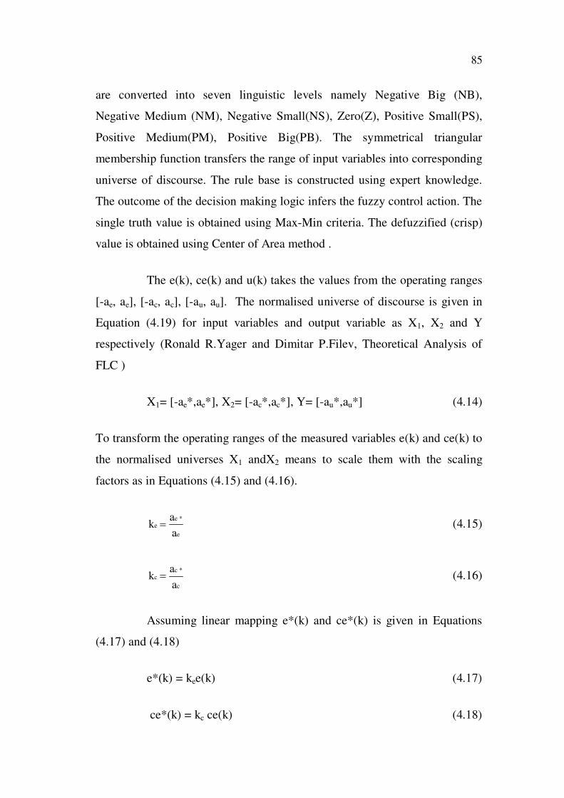
The e(k), ce(k) and u(k) takes the values from the operating ranges

[-ae, ae], [-ac, ac], [-au, au]. The normalised universe of discourse is given in

Equation (4.19) for input variables and output variable as X1, X2 and Y

respectively (Ronald R.Yager and Dimitar P.Filev, Theoretical Analysis of

FLC )

X1= [-ae*,ae*], X2= [-ac*,ac*], Y= [-au*,au*] (4.14)

To transform the operating ranges of the measured variables e(k) and ce(k) to

the normalised universes X1 andX2 means to scale them with the scaling

factors as in Equations (4.15) and (4.16).

e *e

e

ak

a (4.15)

c *c

c

ak

a (4.16)

Assuming linear mapping e*(k) and ce*(k) is given in Equations

(4.17) and (4.18)

e*(k) = kee(k) (4.17)

ce*(k) = kc ce(k) (4.18)

86

Defuzzified value u*(k), obtained by the application of the FLC

algorithm, belongs to the normalised universe Y = [-au*, au*] and related to

the real change of control variable u(k) from the operating range [-au*,au*]

through the scaling factor ku as in Equation (4.19) .

u *u

u

ak

a (4.19)

By applying the normalised value of the input and output values e*(k), ce*(k)

and u*(k) of the input and output variables, we get

u*(k) = kp ce*(k) + kI e*(k) (4.20)

Using the scaling factor, the Equation (4.20) becomes

p c I e

u

u(k)k ce(k)k k e(k)k

k (4.21)

Simplifying the Equation (4.21)

u(k) = kp ce(k) (kc ku)+ kI e(k)( ke ku) (4.22)

Thus FLC is approximated as PI tuned FLC controller as given in Equation

(4.23)

u(k) = KP ce(k)+ KI e(k) (4.23)

Where KP = kp kc ku

KI = kI ke ku

The Table 4.7 gives the scaling factor for Fuzzy tuned – PI

controller.

87

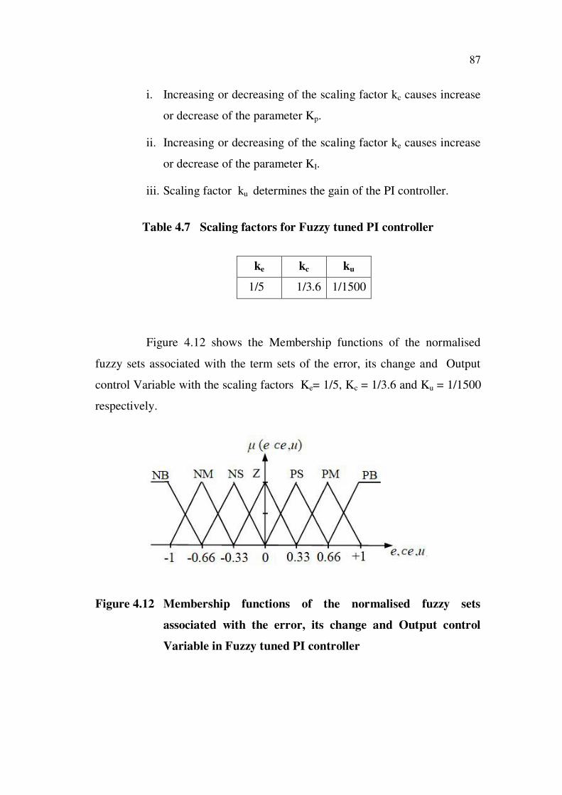
i. Increasing or decreasing of the scaling factor kc causes increase

or decrease of the parameter Kp.

ii. Increasing or decreasing of the scaling factor ke causes increase

or decrease of the parameter KI.

iii. Scaling factor ku determines the gain of the PI controller.

Table 4.7 Scaling factors for Fuzzy tuned PI controller

ke kc ku

1/5 1/3.6 1/1500

Figure 4.12 shows the Membership functions of the normalised

fuzzy sets associated with the term sets of the error, its change and Output

control Variable with the scaling factors Ke= 1/5, Kc = 1/3.6 and Ku = 1/1500

respectively.

Figure 4.12 Membership functions of the normalised fuzzy sets

associated with the error, its change and Output control

Variable in Fuzzy tuned PI controller

88

4.3.3.2 Closed loop simulation using Fuzzy tuned PI control scheme

The closed loop response of PMBLDC motor with Fuzzy tuned PI

controller for set point changes in speed is shown in Figure 4.13. The

variation in actual speed of PMBLDC motor for changes in set values is

shown. When the set speed is slowly changed from 0 to 200 rpm and then to

1500 rpm, the motor speed also reaches the set value due to PI controller

action.

The corresponding variation of line voltage applied to the stator

coil of PMBLDC motor is as in Figure 4.13. At t = 5.0 seconds the motor

speed is increased from 200 rpm to 1500 rpm. It is clearly seen from Figure

4.13 that there is an increase in line voltage at t = 5.0 seconds due to

controller action and the rotor reaches the speed 1500 rpm at t = 5.5 seconds.

Figure 4.13 Closed loop response of PMBLDC motor with Fuzzy tuned

PI controller scheme for set point Tracking

89

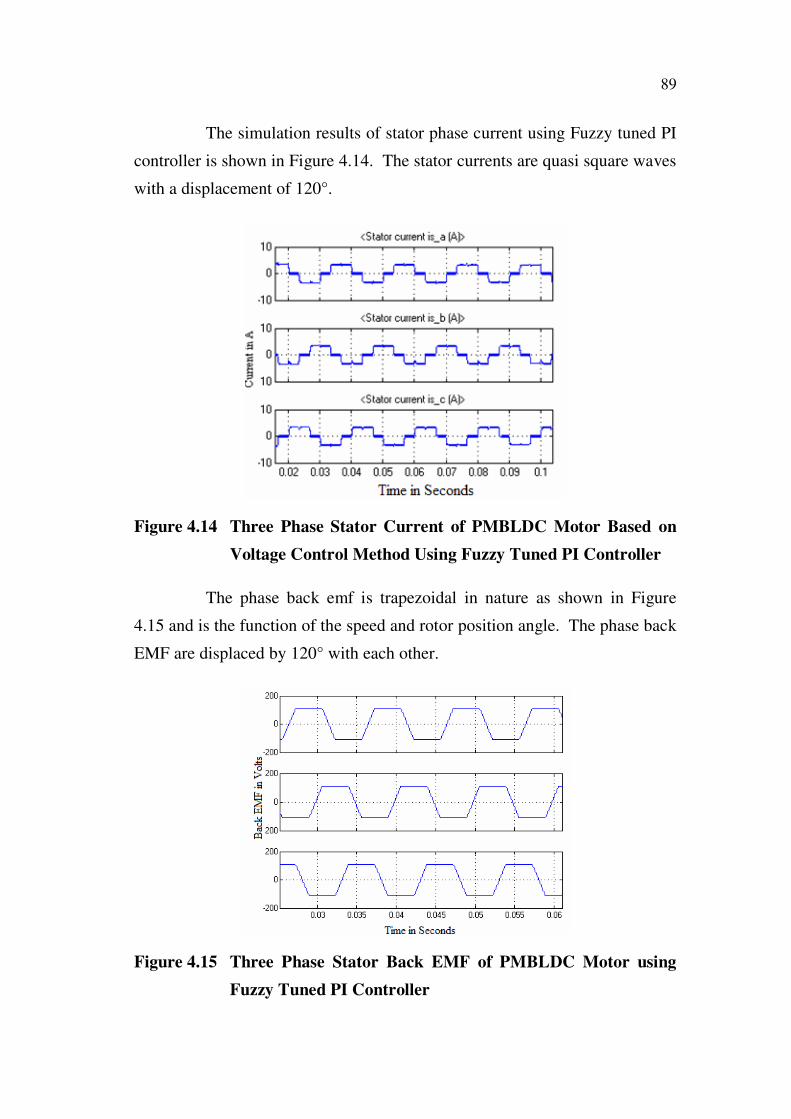
The simulation results of stator phase current using Fuzzy tuned PI

controller is shown in Figure 4.14. The stator currents are quasi square waves

with a displacement of 120°.

Figure 4.14 Three Phase Stator Current of PMBLDC Motor Based on

Voltage Control Method Using Fuzzy Tuned PI Controller

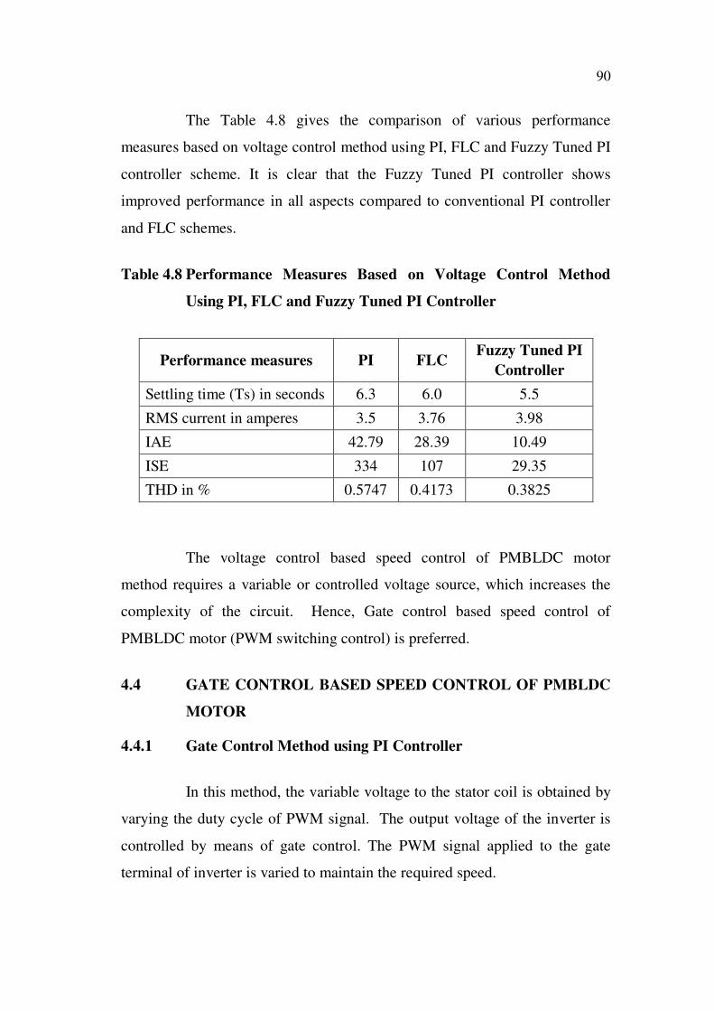
The phase back emf is trapezoidal in nature as shown in Figure

4.15 and is the function of the speed and rotor position angle. The phase back

EMF are displaced by 120° with each other.

Figure 4.15 Three Phase Stator Back EMF of PMBLDC Motor using

Fuzzy Tuned PI Controller

90

The Table 4.8 gives the comparison of various performance

measures based on voltage control method using PI, FLC and Fuzzy Tuned PI

controller scheme. It is clear that the Fuzzy Tuned PI controller shows

improved performance in all aspects compared to conventional PI controller

and FLC schemes.

Table 4.8 Performance Measures Based on Voltage Control Method

Using PI, FLC and Fuzzy Tuned PI Controller

Performance measures PI FLCFuzzy Tuned PI

Controller

Settling time (Ts) in seconds 6.3 6.0 5.5

RMS current in amperes 3.5 3.76 3.98

IAE 42.79 28.39 10.49

ISE 334 107 29.35

THD in % 0.5747 0.4173 0.3825

The voltage control based speed control of PMBLDC motor

method requires a variable or controlled voltage source, which increases the

complexity of the circuit. Hence, Gate control based speed control of

PMBLDC motor (PWM switching control) is preferred.

4.4 GATE CONTROL BASED SPEED CONTROL OF PMBLDC

MOTOR

4.4.1 Gate Control Method using PI Controller

In this method, the variable voltage to the stator coil is obtained by

varying the duty cycle of PWM signal. The output voltage of the inverter is

controlled by means of gate control. The PWM signal applied to the gate

terminal of inverter is varied to maintain the required speed.

91

The dc component corresponding to the amplitude IMAX

of the

original phase current is compared with IREF and the obtained error is

processed through PI controller. The output of the PI controller changes the

duty cycle of the PWM signal. The inverter receives the gate pulses from the

PWM Gate block. The output of the inverter is fed as stator phase voltage.

By controlling the stator phase voltage, the stator phase current varies, thus

controlling the speed of a motor.

Similar to the voltage control method, the position sensing for a

PMBLDC motor needs to detect six positions, which determine the

commutation points. The commutation sequence is identified from the stator

phase current. The PWM gate control block receives two inputs, switching

signal from decoder and duty cycle generated from the PI controller block.

Based on the controller output the width of the pulses changes, which inturn

varies the stator voltage of the PMBLDC motor. The motor parameters are

identified from the open loop simulation results of input and output variables

of PMBLDC motors. The controller parameters and were identified

using system identification technique.

The reference dc link current atth

instant is given by Equation(4.24)

(4.24)

Where and are the errors atth

and -1 instants

and are the dc link reference currents atth

and -1 instants. and are the proportional and Integral gains.

92

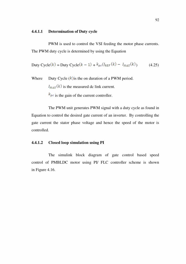
4.4.1.1 Determination of Duty cycle

PWM is used to control the VSI feeding the motor phase currents.

The PWM duty cycle is determined by using the Equation

Duty Cycle = Duty Cycle + ) (4.25)

Where Duty Cycle ( is the on duration of a PWM period.

is the measured dc link current.

is the gain of the current controller.

The PWM unit generates PWM signal with a duty cycle as found in

Equation to control the desired gate current of an inverter. By controlling the

gate current the stator phase voltage and hence the speed of the motor is

controlled.

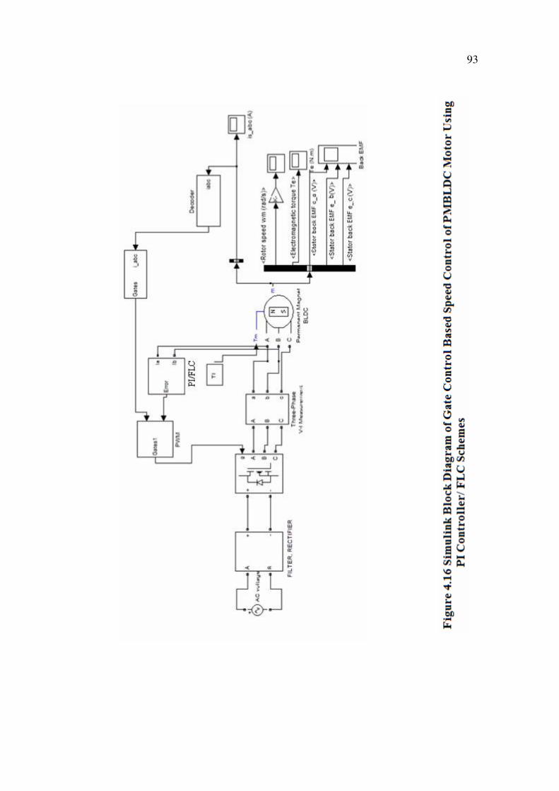
4.4.1.2 Closed loop simulation using PI

The simulink block diagram of gate control based speed

control of PMBLDC motor using PI/ FLC controller scheme is shown

in Figure 4.16.

93

94

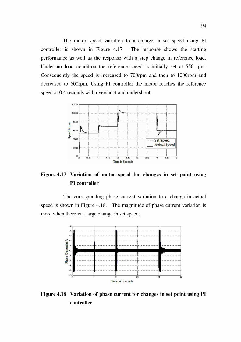
The motor speed variation to a change in set speed using PI

controller is shown in Figure 4.17. The response shows the starting

performance as well as the response with a step change in reference load.

Under no load condition the reference speed is initially set at 550 rpm.

Consequently the speed is increased to 700rpm and then to 1000rpm and

decreased to 600rpm. Using PI controller the motor reaches the reference

speed at 0.4 seconds with overshoot and undershoot.

Figure 4.17 Variation of motor speed for changes in set point using

PI controller

The corresponding phase current variation to a change in actual

speed is shown in Figure 4.18. The magnitude of phase current variation is

more when there is a large change in set speed.

Figure 4.18 Variation of phase current for changes in set point using PI

controller

95

The corresponding electromagnetic torque variation to a

change in actual speed is shown in Figure 4.19. When the set speed is

decreased from 1000 rpm to 600 rpm the variation in torque is in negative

direction as shown in Figure 4.19.

Figure 4.19 Variation of electromagnetic torque for changes in

set point using PI controller

Figure 4.20 shows the speed response of the PMBLDC drive for

changes in set point with constant load torque of 5N-m using PI controller.

There is an overshoot in the speed response and it takes more settling time to

reach the actual speed.

Figure 4.20 Variation of motor speed for changes in set point with

constant load using PI controller

96

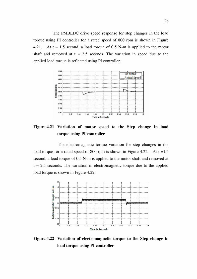
The PMBLDC drive speed response for step changes in the load

torque using PI controller for a rated speed of 800 rpm is shown in Figure

4.21. At t = 1.5 second, a load torque of 0.5 N-m is applied to the motor

shaft and removed at t = 2.5 seconds. The variation in speed due to the

applied load torque is reflected using PI controller.

Figure 4.21 Variation of motor speed to the Step change in load

torque using PI controller

The electromagnetic torque variation for step changes in the

load torque for a rated speed of 800 rpm is shown in Figure 4.22. At t =1.5

second, a load torque of 0.5 N-m is applied to the motor shaft and removed at

t = 2.5 seconds. The variation in electromagnetic torque due to the applied

load torque is shown in Figure 4.22.

Figure 4.22 Variation of electromagnetic torque to the Step change in

load torque using PI controller

97

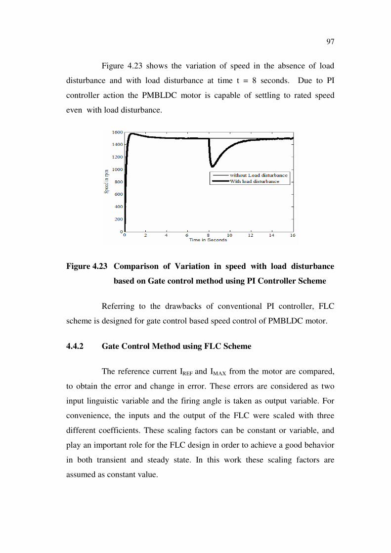
Figure 4.23 shows the variation of speed in the absence of load

disturbance and with load disturbance at time t = 8 seconds. Due to PI

controller action the PMBLDC motor is capable of settling to rated speed

even with load disturbance.

Figure 4.23 Comparison of Variation in speed with load disturbance

based on Gate control method using PI Controller Scheme

Referring to the drawbacks of conventional PI controller, FLC

scheme is designed for gate control based speed control of PMBLDC motor.

4.4.2 Gate Control Method using FLC Scheme

The reference current IREF and IMAX from the motor are compared,

to obtain the error and change in error. These errors are considered as two

input linguistic variable and the firing angle is taken as output variable. For

convenience, the inputs and the output of the FLC were scaled with three

different coefficients. These scaling factors can be constant or variable, and

play an important role for the FLC design in order to achieve a good behavior

in both transient and steady state. In this work these scaling factors are

assumed as constant value.

98

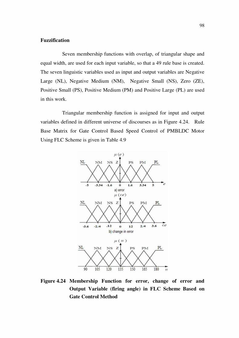
Fuzzification

Seven membership functions with overlap, of triangular shape and

equal width, are used for each input variable, so that a 49 rule base is created.

The seven linguistic variables used as input and output variables are Negative

Large (NL), Negative Medium (NM), Negative Small (NS), Zero (ZE),

Positive Small (PS), Positive Medium (PM) and Positive Large (PL) are used

in this work.

Triangular membership function is assigned for input and output

variables defined in different universe of discourses as in Figure 4.24. Rule

Base Matrix for Gate Control Based Speed Control of PMBLDC Motor

Using FLC Scheme is given in Table 4.9

Figure 4.24 Membership Function for error, change of error and

Output Variable (firing angle) in FLC Scheme Based on

Gate Control Method

99

The error is defined in Equation (4.26) as

e(k) = y(k) –w(k) (4.26)

Where e(k) is the error

w(k) is the Ref current

y(k) is the Actual current

The change in error is defined in Equation (4.27)

ce(k) = e(k) –e(k-1) (4.27)

Table 4.9 Rule Base Matrix for Gate Control Based Speed Control of

PMBLDC Motor Using FLC Scheme

e(k)/

ce(k)PL PM PS Z NS NM NL

PL NL NL NL NL NM NS Z

PM NL NL NM NM NS Z PS

PS NL NM NS NS Z PS PM

Z NM NM NS Z PS PM PM

NS NM NS Z PS PS PM PL

NM NS Z PS PM PM PL PL

NL Z PS PM PL PL PL PL

Decision making logic

‘Max-Min’ criterion is used to combine the results to generate

single truth value, which determines the outcome of the rules.

Defuzzification

The Defuzzification using Center of Area is considered for this

application as it produces the results which are sensitive to all the rules. FLC

design parameters for the gate control based speed control of PMBLDC motor

is given in Table 4.10.

100

Table 4.10 FLC Design Parameters for the Gate Control Based Speed

Control of PMBLDC Motor

Parameters Values

Input variables 2

Output variable 1

linguistic levels 7

Rules 49

Membership Function Triangular

Decision making logic Max-Min criteria

Defuzzification Centre of Area method

4.4.2.1 Closed loop simulation using FLC Scheme

The closed loop simulation results of stator phase current and phase

back EMF using Gate controlled based FLC scheme is shown in Figure 4.25.

The phase back- Emf is in phase with stator phase current. In order to get

maximum efficiency from the motor, the commutation should take place

when the current in a stator winding is in phase with the back EMF of the

same winding. The maximum efficiency is obtained only when the phase back

EMF and stator current are in phase as in Figure 4.25.

Figure 4.25 Phase back- EMF and Stator Current Variation in PMBLDC

Motor Based on Gate Control Method Using FLC Scheme

101

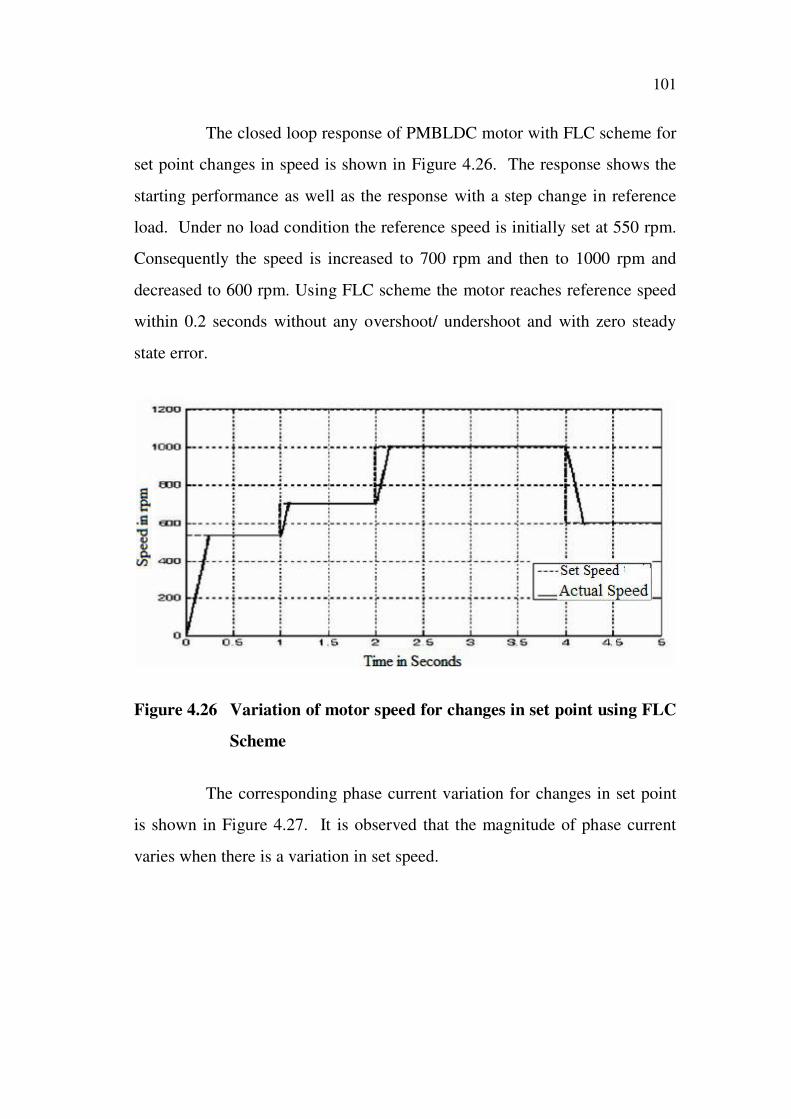
The closed loop response of PMBLDC motor with FLC scheme for

set point changes in speed is shown in Figure 4.26. The response shows the

starting performance as well as the response with a step change in reference

load. Under no load condition the reference speed is initially set at 550 rpm.

Consequently the speed is increased to 700 rpm and then to 1000 rpm and

decreased to 600 rpm. Using FLC scheme the motor reaches reference speed

within 0.2 seconds without any overshoot/ undershoot and with zero steady

state error.

Figure 4.26 Variation of motor speed for changes in set point using FLC

Scheme

The corresponding phase current variation for changes in set point

is shown in Figure 4.27. It is observed that the magnitude of phase current

varies when there is a variation in set speed.

102

Figure 4.27 Variation of phase current for changes in set point using

FLC Scheme

The corresponding electromagnetic torque variation to a change in

set point is shown in Figure 4.28. When the set speed is decreased from

1000rpm to 600rpm the variation in torque is in negative direction.

Figure 4.28 Variation of electromagnetic torque for changes in set

point using FLC Scheme

103

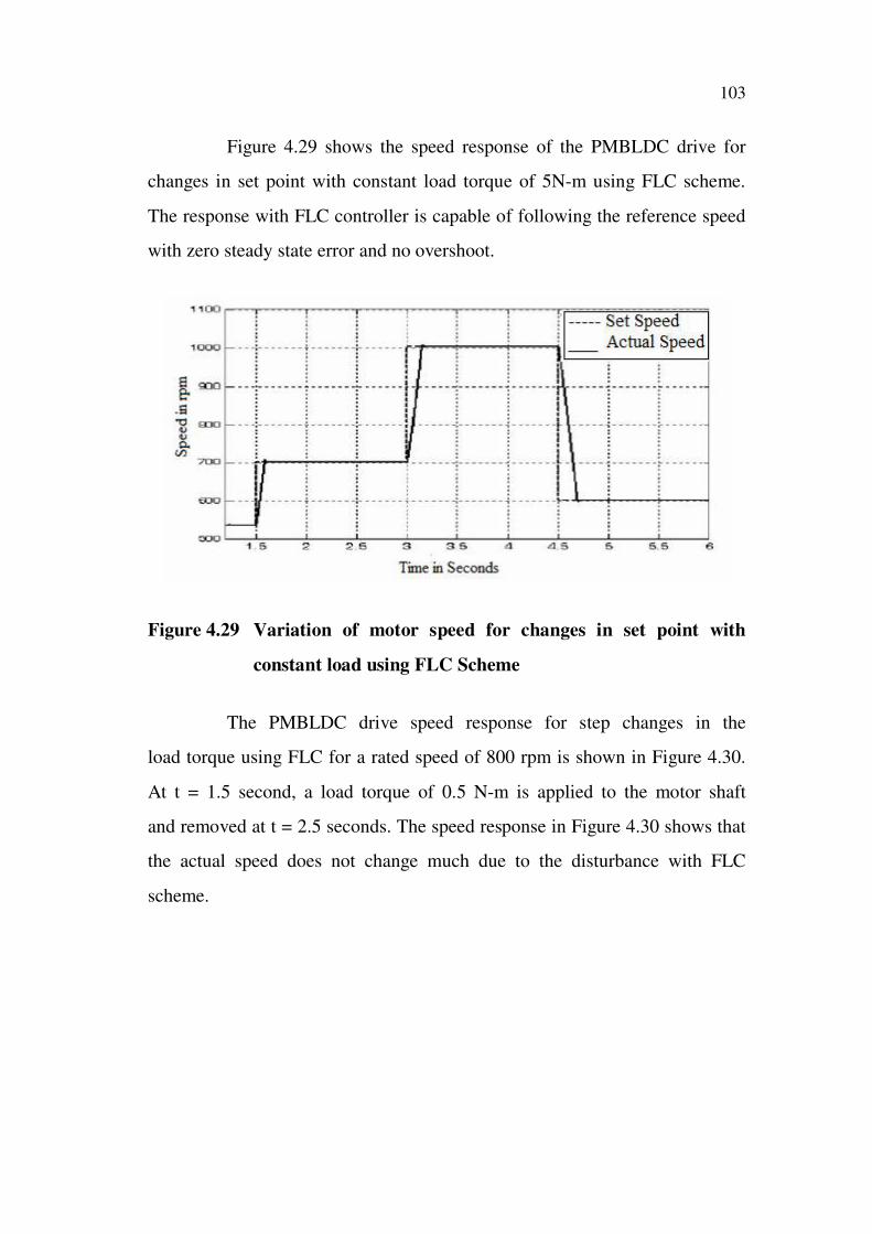
Figure 4.29 shows the speed response of the PMBLDC drive for

changes in set point with constant load torque of 5N-m using FLC scheme.

The response with FLC controller is capable of following the reference speed

with zero steady state error and no overshoot.

Figure 4.29 Variation of motor speed for changes in set point with

constant load using FLC Scheme

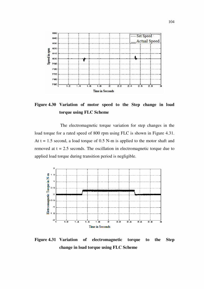
The PMBLDC drive speed response for step changes in the

load torque using FLC for a rated speed of 800 rpm is shown in Figure 4.30.

At t = 1.5 second, a load torque of 0.5 N-m is applied to the motor shaft

and removed at t = 2.5 seconds. The speed response in Figure 4.30 shows that

the actual speed does not change much due to the disturbance with FLC

scheme.

104

Figure 4.30 Variation of motor speed to the Step change in load

torque using FLC Scheme

The electromagnetic torque variation for step changes in the

load torque for a rated speed of 800 rpm using FLC is shown in Figure 4.31.

At t = 1.5 second, a load torque of 0.5 N-m is applied to the motor shaft and

removed at t = 2.5 seconds. The oscillation in electromagnetic torque due to

applied load torque during transition period is negligible.

Figure 4.31 Variation of electromagnetic torque to the Step

change in load torque using FLC Scheme

105

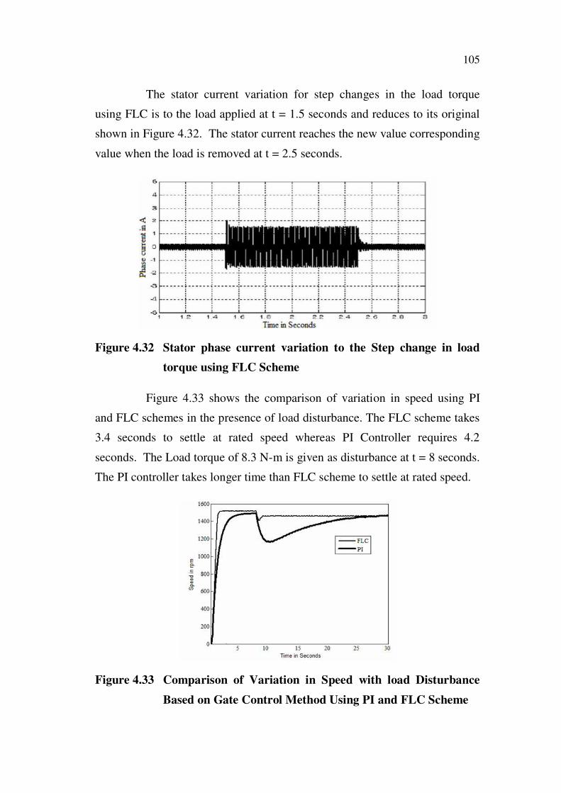
The stator current variation for step changes in the load torque

using FLC is to the load applied at t = 1.5 seconds and reduces to its original

shown in Figure 4.32. The stator current reaches the new value corresponding

value when the load is removed at t = 2.5 seconds.

Figure 4.32 Stator phase current variation to the Step change in load

torque using FLC Scheme

Figure 4.33 shows the comparison of variation in speed using PI

and FLC schemes in the presence of load disturbance. The FLC scheme takes

3.4 seconds to settle at rated speed whereas PI Controller requires 4.2

seconds. The Load torque of 8.3 N-m is given as disturbance at t = 8 seconds.

The PI controller takes longer time than FLC scheme to settle at rated speed.

Figure 4.33 Comparison of Variation in Speed with load Disturbance

Based on Gate Control Method Using PI and FLC Scheme

106

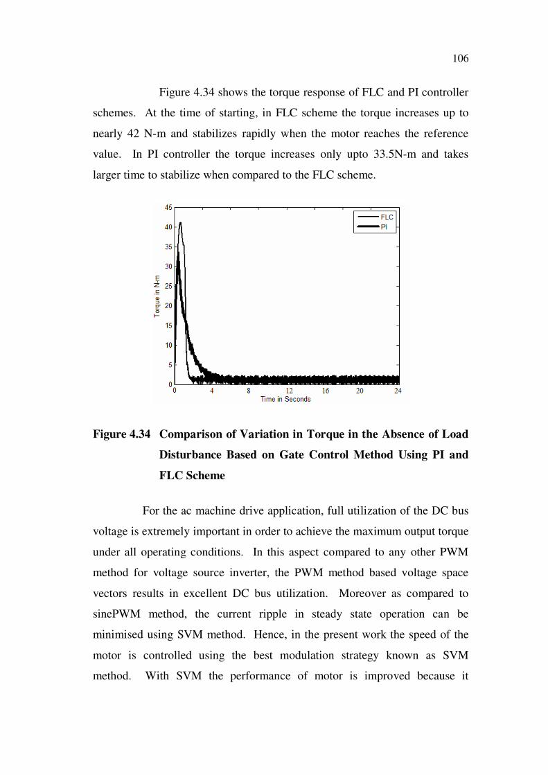
Figure 4.34 shows the torque response of FLC and PI controller

schemes. At the time of starting, in FLC scheme the torque increases up to

nearly 42 N-m and stabilizes rapidly when the motor reaches the reference

value. In PI controller the torque increases only upto 33.5N-m and takes

larger time to stabilize when compared to the FLC scheme.

Figure 4.34 Comparison of Variation in Torque in the Absence of Load

Disturbance Based on Gate Control Method Using PI and

FLC Scheme

For the ac machine drive application, full utilization of the DC bus

voltage is extremely important in order to achieve the maximum output torque

under all operating conditions. In this aspect compared to any other PWM

method for voltage source inverter, the PWM method based voltage space

vectors results in excellent DC bus utilization. Moreover as compared to

sinePWM method, the current ripple in steady state operation can be

minimised using SVM method. Hence, in the present work the speed of the

motor is controlled using the best modulation strategy known as SVM

method. With SVM the performance of motor is improved because it

107

eliminates all the lower order harmonics in the output voltage of the inverter.

The performance of the motor can be further improved by eliminating the

current harmonics in the stator current of the motor. When the machine is on

load, the load neutral is isolated, which causes interaction among phases.

Since, interaction was not considered; stator current harmonics could not be

reduced in the Gate control method. In order to overcome the above

drawbacks, the SVM method is proposed.

4.4.3 Space Vector Modulation (SVM)

SVM is a digital modulating technique, where the objective is to

generate PWM output in such a way that the average voltages follow the

sinusoidal three phase command voltages with a minimum amount of

harmonic distortion. This is done in each sampling period by properly

selecting the switch states of the inverter and by the computation of the

appropriate time period for each state. The SVM for a three phase voltage

source inverter is obtained by sampling the reference vector at the fixed

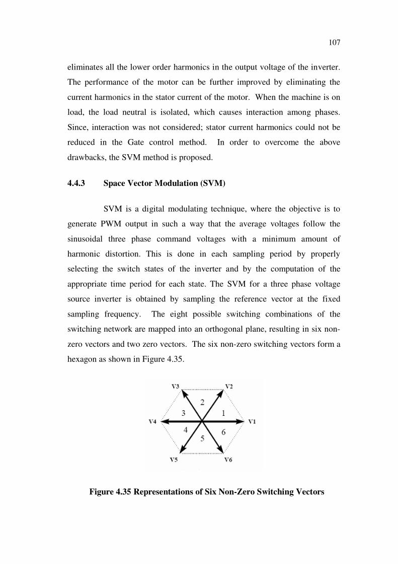
sampling frequency. The eight possible switching combinations of the

switching network are mapped into an orthogonal plane, resulting in six non-

zero vectors and two zero vectors. The six non-zero switching vectors form a

hexagon as shown in Figure 4.35.

Figure 4.35 Representations of Six Non-Zero Switching Vectors

108

In order to implement the SVPWM, the voltage equations in the a-

b-c reference frame can be transformed into the stationary d-q reference frame

that consists of the horizontal (direct) and vertical (quadrature) axes. There

are eight possible combinations of ON and OFF patterns for the upper power

switches. The ON and OFF states of the lower power devices are opposite to

the upper one and hence are easily determined, once the states of the upper

power switches are determined.

4.4.3.1 Modulation Procedure

The four steps involved to perform the Space Vector Modulation

are as follows:

1. The reference signals for phase A, B and C are mapped into

the orthogonal d-q co-ordinated and are represented by

reference vector Vref.

2. Switching vectors are selected, including non-zero and zero

vectors to synthesize the reference vector Vref for one

switching cycle.

3. The time durations for all selected switching vectors are

calculated by a simple trigonometric algorithm. The objective

is to make the averaged switching vector in one switching

cycle equal to the reference vector Vref.

4. The switching vectors are sequenced and applied to the

switching network.

4.4.3.2 Modulation Algorithm

The various steps involved in the modulation algorithm is as follows:

1. Read three phase reference voltages (Va, Vb, Vc).

109

2. Obtain three-phase to two-phase transformation (a, b, c d,

q).

3. Calculate absolute values of Vd, Vq and arc-tangent (Vd/Vq).

4. Identify the sector in which the reference voltage vector lies.

5. Select the switching vectors corresponding to the identified

sector.

6. The switching times are calculated depending on the output

voltage vector magnitude.

7. Sequence the switching vectors as given by the sequencing

scheme (symmetrical).

8. Control signals are applied for each phase of the switching

network.

9. Output is obtained at the load terminals of the voltage source

inverter.

The relationship between the switching variable vector (a, b, c)t and

the line-to-line voltage vectors (Vab, Vbc, Vca)t is given in Equation (4.28)

c

b

a

101

110

011

V

V

V

V

dc

ca

bc

ab

(4.28)

Also, the relationship between the switching variable vector (a, b, c)t

and the phase voltage vector (Van, Vbn, Vcn)t can be expressed as given in

Equation (4.29).

c

b

a

211

121

112

3

V

V

V

Vdc

cn

bn

an

(4.29)

110

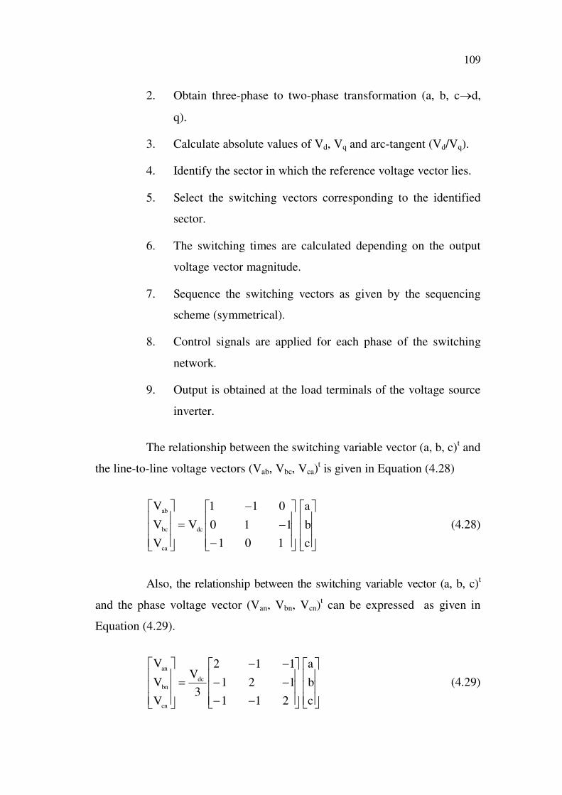
There are six modes of operation in a cycle and the duration of each

mode is 60o. The switches are numbered in the sequence of gating them

(612, 123, 234, 345, 456 and 561). The line to neutral and line to line voltages

in terms of dc-link voltage Vdc obtained for the eight switching vectors using

Equations (4.28) and (4.29) are presented in Table 4.11.

Table 4.11 Voltages across the switching vectors

Switching VectorsLine to Neutral

VoltageLine to line VoltageVoltage

Vectora b c Van Vbn Vcn Vab Vbc Vca

V1 1 0 0 2/3 -1/3 -1/3 1 0 -1

V2 1 1 0 1/3 1/3 -2/3 0 1 -1

V3 0 1 0 -1/3 2/3 -1/3 -1 1 0

V4 0 1 1 -2/3 1/3 1/3 -1 0 1

V5 0 0 1 -1/3 -1/3 2/3 0 -1 1

V6 1 0 1 1/3 -2/3 1/3 1 -1 0

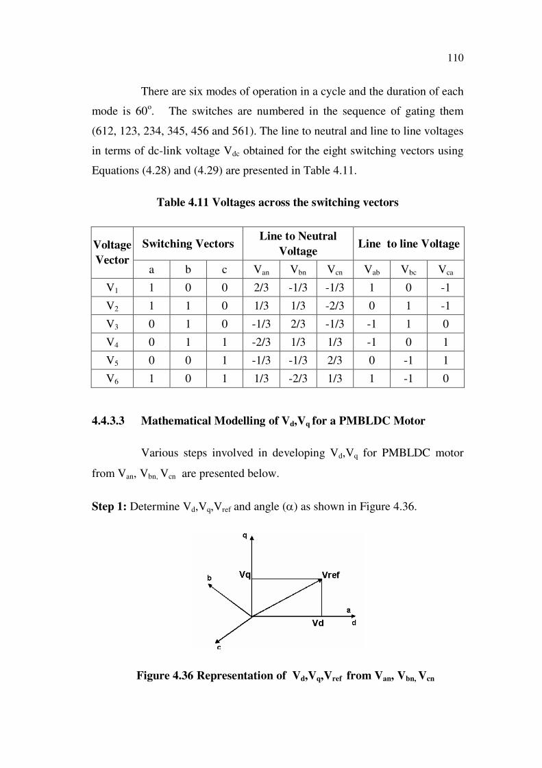
4.4.3.3 Mathematical Modelling of Vd,Vq for a PMBLDC Motor

Various steps involved in developing Vd,Vq for PMBLDC motor

from Van, Vbn, Vcn are presented below.

Step 1: Determine Vd,Vq,Vref and angle ( ) as shown in Figure 4.36.

Figure 4.36 Representation of Vd,Vq,Vref from Van, Vbn, Vcn

111

Vd = Van – Vbn Cos 60o – Vcn Cos 60

o

= Van-1/2Vbn-1/2Vcn (4.30)

Vq = 0 + Vbn Cos 30o – Vcn Cos 30

o

= 3/2 Vbn 3/2Vcn (4.31)

From the above Equations (4.30) and (4.31), the relationship

between direct voltage (Vd) and Quadrature voltage (Vq) with line to neutral

voltage is given in Equation (4.32)

(4.32)

Vref Vd2 + Vq

2 (4.33)

(4.34)

Step 2: Determine the time duration T1, T2 and T0

Figure 4.37 Reference Vector Realization at Sector1

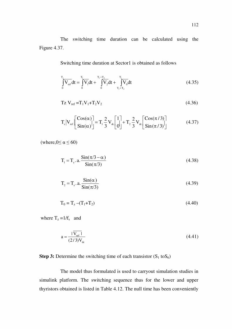
112

The switching time duration can be calculated using the

Figure 4.37.

Switching time duration at Sector1 is obtained as follows

1 z

21

21z T

0

T

TT

0

TT

0

21

T

0

refdtVdtVdtVdtV (4.35)

Tz Vref =T1V1+T2V2 (4.36)

)3/(Sin

)3/(CosV

3

2T

0

1V

3

2T

)(Sin

)(CosVT

dc2dc1refz (4.37)

(where,0 60)

)Sin(

Sin(a..TT

z1 (4.38)

)Sin(

Sin(a..TT

z2 (4.39)

T0 = Tz –(T1+T2) (4.40)

where Tz =1/fs and

dc

ref

V)3/2(

|V|a (4.41)

Step 3: Determine the switching time of each transistor (S1 toS6)

The model thus formulated is used to carryout simulation studies in

simulink platform. The switching sequence thus for the lower and upper

thyristors obtained is listed in Table 4.12. The null time has been conveniently

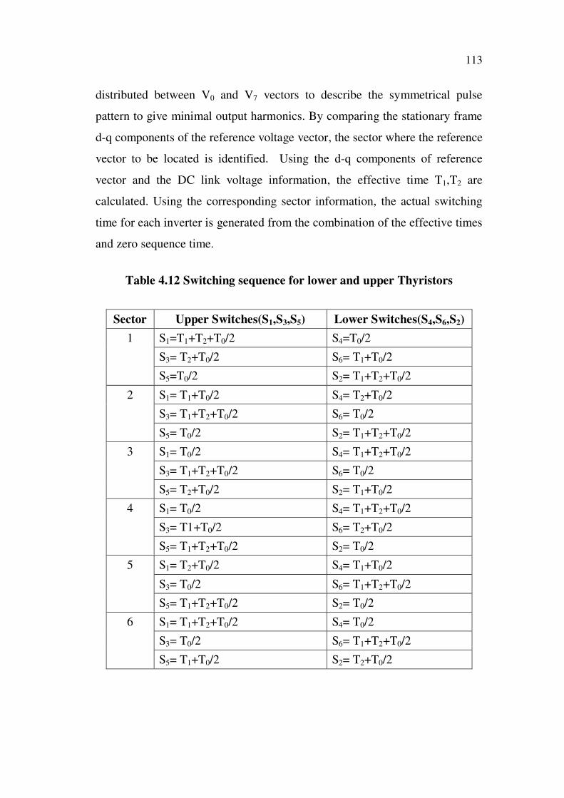
113

distributed between V0 and V7 vectors to describe the symmetrical pulse

pattern to give minimal output harmonics. By comparing the stationary frame

d-q components of the reference voltage vector, the sector where the reference

vector to be located is identified. Using the d-q components of reference

vector and the DC link voltage information, the effective time T1,T2 are

calculated. Using the corresponding sector information, the actual switching

time for each inverter is generated from the combination of the effective times

and zero sequence time.

Table 4.12 Switching sequence for lower and upper Thyristors

Sector Upper Switches(S1,S3,S5) Lower Switches(S4,S6,S2)

S1=T1+T2+T0/2 S4=T0/2

S3= T2+T0/2 S6= T1+T0/2

1

S5=T0/2 S2= T1+T2+T0/2

S1= T1+T0/2 S4= T2+T0/2

S3= T1+T2+T0/2 S6= T0/2

2

S5= T0/2 S2= T1+T2+T0/2

S1= T0/2 S4= T1+T2+T0/2

S3= T1+T2+T0/2 S6= T0/2

3

S5= T2+T0/2 S2= T1+T0/2

S1= T0/2 S4= T1+T2+T0/2

S3= T1+T0/2 S6= T2+T0/2

4

S5= T1+T2+T0/2 S2= T0/2

S1= T2+T0/2 S4= T1+T0/2

S3= T0/2 S6= T1+T2+T0/2

5

S5= T1+T2+T0/2 S2= T0/2

S1= T1+T2+T0/2 S4= T0/2

S3= T0/2 S6= T1+T2+T0/2

6

S5= T1+T0/2 S2= T2+T0/2

114

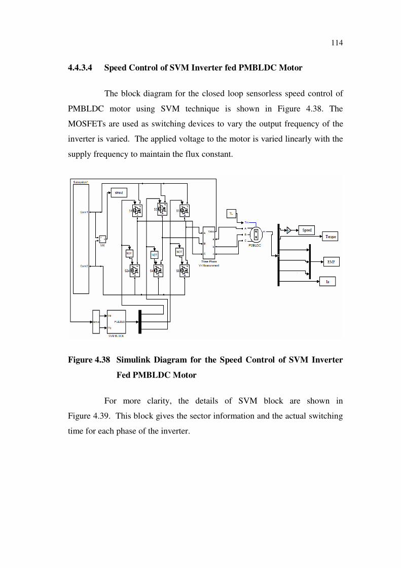
4.4.3.4 Speed Control of SVM Inverter fed PMBLDC Motor

The block diagram for the closed loop sensorless speed control of

PMBLDC motor using SVM technique is shown in Figure 4.38. The

MOSFETs are used as switching devices to vary the output frequency of the

inverter is varied. The applied voltage to the motor is varied linearly with the

supply frequency to maintain the flux constant.

Figure 4.38 Simulink Diagram for the Speed Control of SVM Inverter

Fed PMBLDC Motor

For more clarity, the details of SVM block are shown in

Figure 4.39. This block gives the sector information and the actual switching

time for each phase of the inverter.

115

Figure 4.39 Simulink Diagram for Determining Sector and Switching

Duration in SVM Block

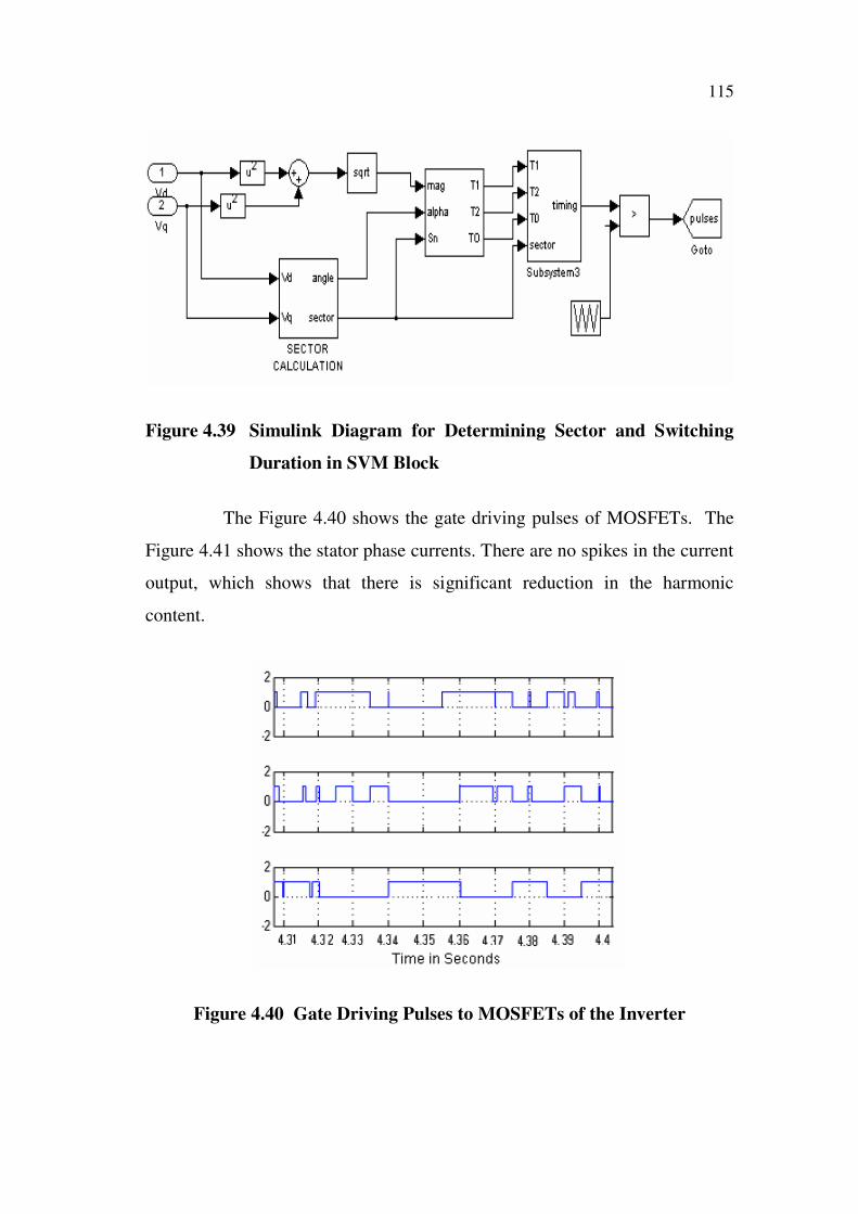
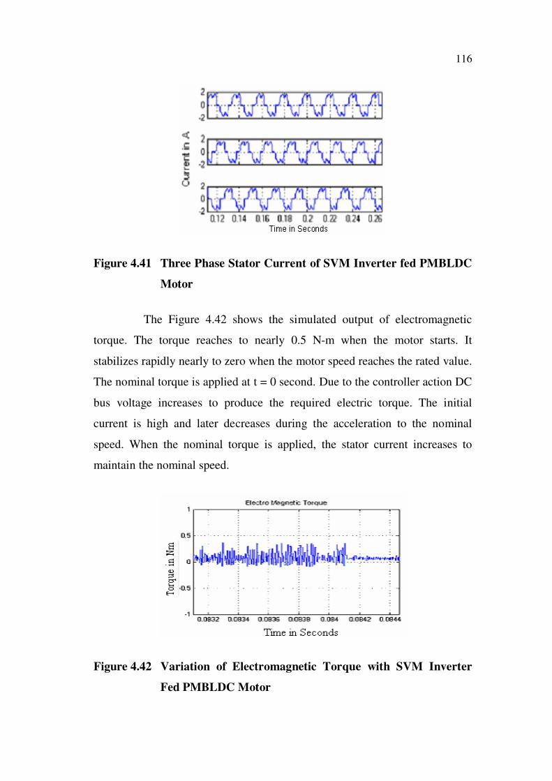
The Figure 4.40 shows the gate driving pulses of MOSFETs. The

Figure 4.41 shows the stator phase currents. There are no spikes in the current

output, which shows that there is significant reduction in the harmonic

content.

Figure 4.40 Gate Driving Pulses to MOSFETs of the Inverter

116

Figure 4.41 Three Phase Stator Current of SVM Inverter fed PMBLDC

Motor

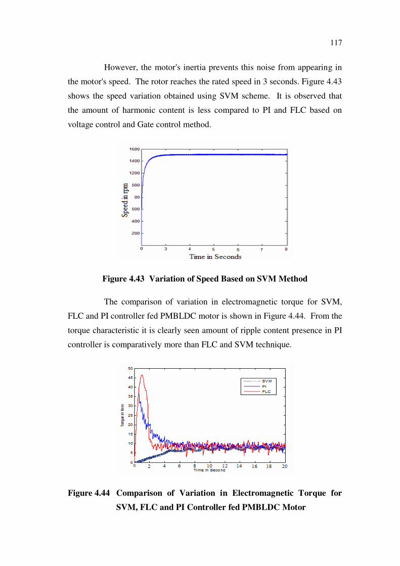
The Figure 4.42 shows the simulated output of electromagnetic

torque. The torque reaches to nearly 0.5 N-m when the motor starts. It

stabilizes rapidly nearly to zero when the motor speed reaches the rated value.

The nominal torque is applied at t = 0 second. Due to the controller action DC

bus voltage increases to produce the required electric torque. The initial

current is high and later decreases during the acceleration to the nominal

speed. When the nominal torque is applied, the stator current increases to

maintain the nominal speed.

Figure 4.42 Variation of Electromagnetic Torque with SVM Inverter

Fed PMBLDC Motor

117

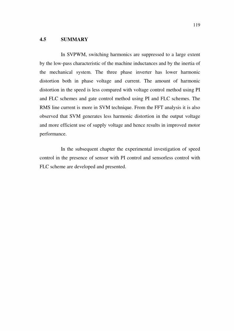
However, the motor's inertia prevents this noise from appearing in

the motor's speed. The rotor reaches the rated speed in 3 seconds. Figure 4.43

shows the speed variation obtained using SVM scheme. It is observed that

the amount of harmonic content is less compared to PI and FLC based on

voltage control and Gate control method.

Figure 4.43 Variation of Speed Based on SVM Method

The comparison of variation in electromagnetic torque for SVM,

FLC and PI controller fed PMBLDC motor is shown in Figure 4.44. From the

torque characteristic it is clearly seen amount of ripple content presence in PI

controller is comparatively more than FLC and SVM technique.

Figure 4.44 Comparison of Variation in Electromagnetic Torque for

SVM, FLC and PI Controller fed PMBLDC Motor

118

The amount ripple content in torque for the SVM, FLC and PI

controller is given in Figure 4.45. The amount of ripple content presence

using PI controller is roughly four times greater than SVM technique.

Figure 4.45 Comparison of Ripple Content in Torque for SVM, FLC

and PI Controller Fed PMBLDC Motor

From the quantitative comparison parameter in Table 4.13 it is

clear that the SVM scheme provides better performance compared to other

schemes. The settling time for the PMBLDC motor to settle at rated speed

using SVM is only 3 seconds. The amount of power transferred to the motor

is larger, which indicates lesser power loss in the inverter and more efficient

use of supply voltage.

Table 4.13 Quantitative Analysis of Performance Measures of Various

Controllers in Sensorless Method

Performance Measures PI ControlFuzzy Logic

Control

Space Vector

Modulation

Settling Time Ts in Second 4.2 3.4 3.0

RMS values of current in Amphere 4.625 4.886 7.35

IAE 69.74 11.55 0.335

ISE 150 33.5 0.8002

THD in % 3.123 1.434 0.2897

119

4.5 SUMMARY

In SVPWM, switching harmonics are suppressed to a large extent

by the low-pass characteristic of the machine inductances and by the inertia of

the mechanical system. The three phase inverter has lower harmonic

distortion both in phase voltage and current. The amount of harmonic

distortion in the speed is less compared with voltage control method using PI

and FLC schemes and gate control method using PI and FLC schemes. The

RMS line current is more in SVM technique. From the FFT analysis it is also

observed that SVM generates less harmonic distortion in the output voltage

and more efficient use of supply voltage and hence results in improved motor

performance.

In the subsequent chapter the experimental investigation of speed

control in the presence of sensor with PI control and sensorless control with

FLC scheme are developed and presented.