CHAPTER 4 Models for ECG and RR Interval Processesgari/ecgbook/ch4.pdfP1: Shashi August 24, 2006...

P1: Shashi

August 24, 2006 11:42 Chan-Horizon Azuaje˙Book

C H A P T E R 4

Models for ECG and RR IntervalProcesses

Patrick E. McSharry and Gari D. Clifford

4.1 Introduction

The availability of open-source computational models and simulators can greatlyfacilitate the advancement of cardiovascular research by complementing clinicalstudies.1 Such models provide the researcher with the means of formulating hy-potheses that may be subsequently tested through investigations of both simulatedbiomedical signals and real-world signals obtained from clinical studies. There isa two-way relationship between the development of these models and the explo-ration of biomedical databases obtained from clinical studies. First, researchers canconstruct and evaluate their models using the biomedical signals. Access to thesedatabases facilitates the estimation of important cardiovascular parameters and thecomparison of different models. Second, the ability to simulate realistic signals usingthese models can be used to assess novel biomedical signal processing techniques.In addition, these models can be used to formulate new experimental hypotheses.

The ECG signal describes the electrical activity in the heart and each heartbeattraces the familiar morphology labeled by the P, Q, R, S, and T peaks and troughs.Since the R peak is typically associated with the largest deflection away from thebaseline, this peak is generally taken as a marker for each heartbeat as it is the easiestto locate. As was pointed out in Chapter 3, the correct fiducial point for each heart-beat is the onset of the P wave. However, this point is both difficult to define andlocate and the Q-R interval is often sufficiently short and of low variability that theR peak suffices to give an accurate fiducial marker of cardiac activity. The sequenceof successive times, ti (i = 1, 2, . . . , n), produced by applying a QRS detector (seeChapter 7) to the ECG signal, are transformed into a sequence of RR intervals via

RRi = ti − ti−1 (4.1)

This sequence of RR intervals forms the basis of the RR interval time series orRR tachogram. A corresponding sequence of instantaneous heart rates may also bedefined by

fi = 1RRi

(4.2)

1. See http://www.physionet.org for a description of available databases and tools.

101

P1: Shashi


102 Models for ECG and RR Interval Processes

In the following sections, a number of useful models and related tools availablefor researchers within the field of biomedical signal processing are described. Thesemodels are grouped into two categories, the first relating to RR intervals and thesecond to ECG signals.

4.2 RR Interval Models

In the following sections, we review a variety of modeling approaches that are use-ful for understanding and investigating the processes underlying the RR tachogram.These models range from physiology-based to empirical data-based approaches andstatistical descriptions that may be used for classification. Section 4.2.1 provides anoverview of the cardiovascular system. Section 4.2.2 gives a summary of the DeBoermodel. Section 4.2.3 discusses a freely available cardiovascular simulator availablefrom PhysioNet. Section 4.2.4 describes the integral pulse frequency modulationmodel. Sections 4.2.5 and 4.2.6 present two data-driven modeling approaches us-ing nonlinear deterministic models and a system of coupled oscillators. A moredescriptive analysis from the point of scale invariance is given in Section 4.2.7. Fi-nally, a selection of models that were entered in the 2002 PhysioNet Challenge aresummarized in Section 4.2.8.

4.2.1 The Cardiovascular System

The cardiovascular system consists of a closed circuit of blood vessels. A continuousmotion of blood from the left to the right heart provides the individual cells withsufficient nutrients. The flow in the vessels is controlled by the myogenic and neuro-genic processes; the former refers to the contraction and relaxation of smooth mus-cle in the vessel wall whereas the latter is driven by the autonomic nervous system.Although the myogenic and neurogenic processes affect heart rate (and hence theECG) over the long term, the dominant observable effects on the RR interval tim-ing and ECG morphology are due to the regulation of the heart’s pacemaker by thesympathetic and parasympathetic branches of the autonomic nervous system (seeChapters 1 and 3). In an oversimplistic sense, the sympathetic nervous system canbe thought of as the body’s fight or flight response, which acts quickly to increaseheart rate, blood pressure, and respiration. Conversely, the parasympathetic systemcan be thought of as the rest and digest system, which acts to slow heart rate (HR)and respiration, as well as lowering blood pressure (BP) (e.g., when falling asleep).

Respiration, a mainly parasympathetically mediated process, is the most obvi-ous observable phenomenon in the RR tachogram (and in the ECG; see Chapter 3and Section 4.3.2). The normal variation in RR intervals (and R amplitudes) ona beat-to-beat basis, known as respiratory sinus arrhythmia [1, 2], is almost syn-chronous with the respiratory oscillations. The small phase differences between thetwo oscillations has been observed to be constant in some circumstances. However,this phase is known to change over even short periods of time, depending on theactivity of the patient (see [3, 4] and Section 4.2.6). There is also a coupling betweenHR and BP and between BP and respiration (see [5] and Section 4.2.2). It shouldbe noted at this point that BP measurements are a function of the location and time

P1: Shashi


4.2 RR Interval Models 103

(in the cycle) at which they are measured. In this chapter, BP refers to the meansystemic arterial pressure (MAP), usually recorded from the brachial artery. Ap-proximately two-thirds of the cardiac cycle is spent in diastole, and therefore MAPis often calculated as one-third of the difference between the maximum and mini-mum aortic pressure following ejection of blood from the left ventricle ( 1

3 systolicBP (SBP) +2

3 diastolic BP (DBP). Pulse pressure is simply the difference between theSBP and the DBP.

Since the effects of the myogenic and neurogenic processes on the RR intervaltime series are not well understood [6], the discussion of the biological processes inthe context of the models presented in this chapter will be confined to short-termcouplings of the cardiovascular system; HR (approximately 0.5 → 5 Hz), respira-tion (approximately 1/15 → 0.5 Hz), and BP (approximately 1/60 → 1/5 Hz).Longer term fluctuations are considered from an empirical standpoint in Sections4.2.7 and 4.2.8 and in Chapter 3.

Any model that describes the changes in RR intervals over time, should allowfor a description of heart rate variability (HRV) and its relationship to HR, BP, andrespiration. There is no simple connection between HR, HRV, and BP. However,many measures of HR and HRV are often inversely correlated: Stimuli that increaseHR often depress the variability of the HR in the short term. Conversely, activitiesthat cause a drop in the average HR can lead to an increase in short-term HRV. Al-though the strength of this correlation can change over time and from individual toindividual, it is useful to consider the cardiovascular system from a static perspectivein order to investigate the relationship between the cardiovascular parameters.

The cardiovascular system may be viewed as a pressure controlled system, andtherefore factors that influence changes in BP will also cause fluctuations in HR. Inresting humans, beat-to-beat fluctuations in BP and HR are mainly due to respira-tory influences and to the slower Mayer waves [5]. Sleight and Casadei [7] emphasizethat there is much evidence to support the idea that beat-to-beat HR variations are amanifestation of a central nervous system oscillator which becomes entrained withrespiration as a result of afferent input from bronchopulmonary receptors.

A variety of approaches have been employed to describe the short-term con-trol of blood pressure. Ottesen et al. [8, 9] provide an excellent review of attemptsat modeling the physiology of the cardiovascular system. Grodins [10] used alge-braic equations for the steady controlled heart which can be rearranged to modelmean arterial pressure by a sixth-order polynomial. Madwed et al. [11] provideda descriptive model using feedback control. Ursino et al. have produced a series ofdifferential delay equation models to allow for changes in the venous capacity andcardiac pulsatility (see [12–14] and references therein). Seidel and Herzel [15] devel-oped a hybrid model with continuous variables and an integrate and fire mechanismto generate a discrete heart rate. McSharry et al. [16] present a simple differentialdelay equation model of the cardiovascular system which is able to reproduce manyof the empirical characteristics observed in biomedical signals such as heart rate,blood pressure, and respiration. The model also includes the effects of RSA, Mayerwaves, and synchronization.

It is generally agreed [7], however, that coupling of HR, respiration, and thecardiac cycle (the flow of blood around the body with its consequent pressures)can be broadly explained as follows: inspiration lowers intrathoracic pressure and

P1: Shashi



enhances filling of the right heart from extrathoracic veins. Right ventricular strokevolume, therefore, increases, and a consequent rise in the effective pressure of therest of the circulation is observed. The rise in effective pressure in the pulmonaryveins leads to an increased filling of the left heart and hence to an increased leftventricular stroke volume.

The resistance and hydraulic capacitances of the lesser circulation create a lagbetween inspiration and right ventricular output increase and between the rise ofeffective pulmonary venous pressure and left ventricular filling. A consequence ofthis is that stroke volume modulation will decrease with increasing respiratory rate(for a given respiratory depth). Furthermore, the phase lag of the stroke volumechange with respect to the corresponding respiratory oscillation will increase forhigher rates. In practice, at moderately rapid respiratory rates, the BP and strokevolume fall throughout most of the inspiration. Therefore, the fall in arterial pres-sure with inspiration is due to the preceding expiration. Furthermore, the strengthof this relationship increases as the patient moves from a supine to upright position.

During expiration, the longer pulse or RR interval buffers any change in dias-tolic pressure caused by the resultant increase in stroke volume, so diastolic pressurechanges may correlate poorly with reflex changes. This supports the notion that res-piration drives BP changes, which in turn drive the RR and HR changes. Diastolic BPchanges with respiration are quite small since the inspiratory tachycardia tends toreduce any inspiratory fall in diastolic pressure (as there is less time for the diastolicpressure to drop).

This observation was first explained by DeBoer in 1987 [5] and although therehave been other mathematical models proposed since then (such as the Baselli model[17] and the Saul model [18]), most experimental evidence is thought to supportDeBoer’s model [7]. For a more detailed survey of the last 50 years of cardiovascularrespiratory modeling, the reader is referred to Batzel et al. [19].

4.2.2 The DeBoer Model

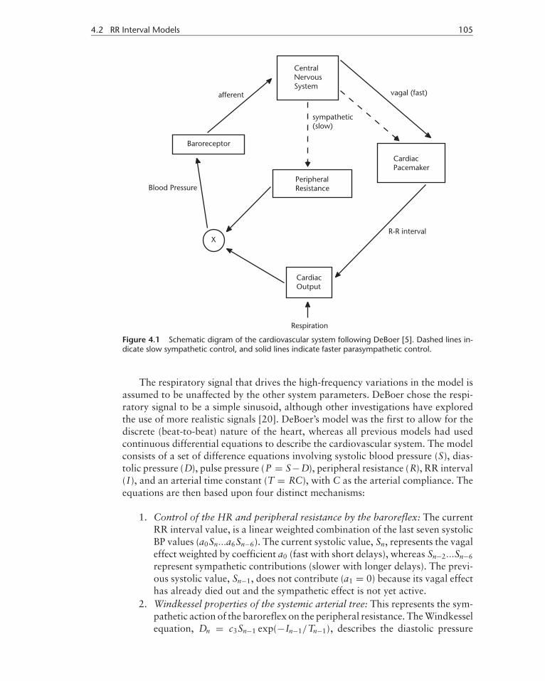
The DeBoer model [5] is a beat-to-beat model of the cardiovascular system de-veloped for investigating the spontaneous short-term variability in arterial BP andHR signals recorded from human subjects at rest. This model explains how the BPaffects both RR interval length and peripheral (capillary) resistance through the ac-tions of the baroreceptors and the central nervous system. Note that slow regulatorymechanisms (< 0.05 Hz) are not included in the model. Figure 4.1 shows how thecardiac output is governed by the current value of respiration and the previous RRinterval. The new BP value is set by this value of cardiac output and the peripheralresistance. The new BP value then determines the new value for the RR interval.Therefore, the model assumes that respiration first affects BP, which in turn affectsthe RR interval. The low-frequency2 peak in HR at 0.1 Hz observed in steady-stateconditions for humans is explained as a resonance phenomenon due to the delay inthe sympathetic control loop of the baroreflex: the reflex sympathetic neural out-flow cannot follow beat-to-beat changes in the BP as sensed by the baroreceptors.

2. See Chapter 3 for an exact definition of the low and high-frequency components.

P1: Shashi



Figure 4.1 Schematic digram of the cardiovascular system following DeBoer [5]. Dashed lines in-dicate slow sympathetic control, and solid lines indicate faster parasympathetic control.

The respiratory signal that drives the high-frequency variations in the model isassumed to be unaffected by the other system parameters. DeBoer chose the respi-ratory signal to be a simple sinusoid, although other investigations have exploredthe use of more realistic signals [20]. DeBoer’s model was the first to allow for thediscrete (beat-to-beat) nature of the heart, whereas all previous models had usedcontinuous differential equations to describe the cardiovascular system. The modelconsists of a set of difference equations involving systolic blood pressure (S), dias-tolic pressure (D), pulse pressure (P = S−D), peripheral resistance (R), RR interval(I), and an arterial time constant (T = RC), with C as the arterial compliance. Theequations are then based upon four distinct mechanisms:

1. Control of the HR and peripheral resistance by the baroreflex: The currentRR interval value, is a linear weighted combination of the last seven systolicBP values (a0Sn...a6Sn−6). The current systolic value, Sn, represents the vagaleffect weighted by coefficient a0 (fast with short delays), whereas Sn−2...Sn−6

represent sympathetic contributions (slower with longer delays). The previ-ous systolic value, Sn−1, does not contribute (a1 = 0) because its vagal effecthas already died out and the sympathetic effect is not yet active.

2. Windkessel properties of the systemic arterial tree: This represents the sym-pathetic action of the baroreflex on the peripheral resistance. The Windkesselequation, Dn = c3Sn−1 exp(−In−1/Tn−1), describes the diastolic pressure

P1: Shashi



decay, governed by the ratio of the previous RR interval to the previousarterial time constant. The time constant of the decay, Tn, and thus (assum-ing a constant arterial compliance C) the current value of the peripheralresistance, Rn, depends on a weighted sum of the previous six values of S.

3. Contractile properties of the myocardium: The influence of the length of theprevious interval on the strength of the ventricular contraction is given byPn = γ In−1 + c2, where γ and c2 are physiological constants. A longer pulseinterval (In−1 > In−2) therefore tends to increase the next pulse pressure(if γ > 0), Pn, a phenomenon motivated by the increased filling of the ven-tricles after a long interval, leading to a more forceful contraction (Starling’slaw) and by the restitution properties of the myocardium (which also leadsto an increased strength of contraction after a longer interval).

4. Mechanical effects of respiration on BP: Respiration is simulated by disturb-ing Pn with a sinusoidal variation in I. Without this addition, the equationsthemselves do not imply any fluctuations in BP or HR but lead to stablevalues for the different variables.

Linearization of the equations of motion around operating points (normal hu-man values for S, D, I, and T) was employed to facilitate an analysis of the model.Note that such a linearization is a good approximation when the subject is at rest.The addition of a simulated respiratory signal was shown to provide a good cor-respondence between the power spectra of real and simulated data. DeBoer alsopointed out the need to perform cross-spectral analysis between the RR tachogram,the systolic BP, and respiration signals. Pitzalis et al. [21] performed such an analy-sis supporting DeBoer’s model and showed that the respiratory rate modulates theinterrelationship between the RR interval and S variabilities: the higher the rate ofrespiration, the smaller the gain and the smaller the phase difference between thetwo. Furthermore, the same response is found after administering a β-adrenoceptorblockade, suggesting that the sympathetic drive is not involved in this process.Sleight and Casadei [7] also present evidence to support the assumptions underly-ing the DeBoer model.

4.2.3 The Research Cardiovascular Simulator

The Research CardioVascular SIMulator (RCVSIM) [22–24] software3 was devel-oped in order to complement the experimental data sets provided by PhysioBank.The human cardiovascular model underlying RCVSIM is based upon an electricalcircuit analog, with charge representing blood volume (Q, ml), current representingblood flow rate (q, ml/s), voltage representing pressure (P, mmHg), capacitance rep-resenting arterial/vascular compliance (C), and resistance (R) representing frictionalresistance to viscous blood flow. RCVSIM includes three major components.

The first component (illustrated in Figure 4.2) is a lumped parameter modelof the pulsatile heart and circulation which itself consists of six compartments,the left ventricles, the right ventricles, the systemic arteries, the systemic veins, the

3. Open-source code and further details are available from http://www.physionet.org/physiotools/rcvsim/.

P1: Shashi



Figure 4.2 PhysioNet’s RCVSIM lumped parameter model of the human heart-lung unit in termsof its electrical circuit analog. Charge is analogous to blood volume (Q, ml), current, to blood flowrate (q, ml/s), and voltage, to pressure (P , mmHg). The model consists of six compartments whichrepresent the left and right ventricles (l ,r ), systemic arteries and veins (a,v), and pulmonary arteriesand veins (pa, pv). Each compartment consists of a conduit for viscous blood flow with resistance(R ), a volume storage element with compliance (C ) and unstressed volume (Q0). The node labeledP”r a”(t) is the location of where the right atrium would be if it were explicitly included in the model.(Adapted from: [22] with permission. c© 2006 R. Mukkamala.)

pulmonary arteries, and the pulmonary veins. Each compartment consists of a con-duit for viscous blood flow with resistance (R), a volume storage element withcompliance (C) and unstressed volume (Q0). The second major component of themodel is a short-term regulatory system based upon the DeBoer model and includesan arterial baroreflex system, a cardiopulmonary baroreflex system, and a directneural coupling mechanism between respiration and heart rate. The third majorcomponent of RCVSIM is a model of resting physiologic perturbations which in-cludes respiration, autoregulation of local vascular beds (exogenous disturbance tosystemic arterial resistance), and higher brain center activity affecting the autonomicnervous system (1/ f exogenous disturbance to heart rate [25]).

The model is capable of generating realistically human pulsatile hemodynamicwaveforms, cardiac function and venous return curves, and beat-to-beat hemody-namic variability. RCVSIM has been previously employed in cardiovascular research

P1: Shashi



by its author for the development and evaluation of system identification methodsaimed at the dynamical characterization of autonomic regulatory mechanisms [23].Recent developments of RCVSIM have involved the development of a parallelizedversion and extensions for adaptation to space-flight data to describe the processesinvolved in orthostatic hypotension [26–28]. Simulink versions have been developedboth with and without the baroreflex reflex mechanism, and an additional intersti-tial compartment to aid work fitting the model parameters to real data representingan instance of hemorrhagic shock [29]. These recent innovations are currently be-ing redeveloped into a platform-independent version which will shortly be availablefrom PhysioNet [22, 30].

4.2.4 Integral Pulse Frequency Modulation Model

The integral pulse frequency modulation (IPFM) model was developed for investi-gating the generation of a discrete series of events, such as a series of heartbeats [31].This model assumes the existence of a continuous-time input modulation signalwhich possesses a particular physiological interpretation, such as describing themechanisms underlying the autonomic nervous system [32]. The action of this mod-ulation signal when integrated through the model generates a series of interbeattime intervals, which may be compared to RR intervals recorded from humansubjects.

The IPFM model assumes that the autonomic activity, including both the sym-pathetic and parasympathetic influences, may be represented by a single modulatinginput signal x(t). This input signal x(t) is integrated until a threshold, R, is reachedwhere a beat is generated. At this point, the integrator is reset to zero and the processis repeated [31, 33] (see Figure 4.3). The beat-to-beat time series may be expressedas a series of pulses,

p(t) = n =∫ tn

0

1 + x(t)T

dt, (4.3)

where n is an integer number representing the nth beat and tn reflects its time stamp.The time T is the mean interbeat interval and x(t)/T is the zero-mean modulatingterm. It is usual to assume that this modulation term is relatively small (x(t) << 1)

Figure 4.3 The integral pulse frequency modulation model. The input signal x(t) is integratedyielding y(t). When y(t) reaches the fixed reference value R, a pulse is emitted and the integratoris reset to 0, whereupon the cycle starts again. Output of the model is the series of pulses p(t).When used to model the cardiac pacemaker, the input is a signal proportional to the acceleratingautonomic efferences on the pacemaker cells and the output is the RR interval time series.

P1: Shashi



in order to reflect that heart rate variability is usually smaller than the mean heartrate. The time-dependent value of (1+ x(t))/T may be viewed as the instantaneousheart rate. For simplification, the first beat is assumed to occur at time t0 = 0.Generally, x(t) is assumed to be band-limited with negligible power for frequenciesgreater than 0.4 Hz.

In physiological terms, the output signal of the integrator can be viewed asthe charging of the membrane potential of a sino-atrial pacemaker cell [34]. Thepotential increases until a certain threshold (R in Figure 4.3) is exceeded and thentriggers an action potential which, when combined with the effect of many otheraction potentials, initiates another cardiac cycle.

Given that the assumptions underlying the IPFM are valid, the aim is to con-struct a method for obtaining information about the input signal x(t) using theobserved sequence of event times tn. The various issues concerning a reasonablechoice of time domain signal for representing the activity in the heart are discussedin [32].

The IPFM model has been extended to provide a time-varying threshold inte-gral pulse frequency modulation (TVTIPFM) model [35]. This approach has beenapplied to RR intervals in order to discriminate between autonomic nervous mod-ulation and the mechanical stretch induced effect caused by changes in the venousreturn and respiratory modulation.

4.2.5 Nonlinear Deterministic Models

A chaotic dynamic system may be capable of generating a wide range of irregulartime series that would normally be associated with stochastic dynamics. The task ofidentifying whether a particular set of observations may have arisen from a chaoticsystem has given rise to a large body of research (see [36] and references therein). Themethod of surrogate data is particularly useful for constructing hypothesis tests forasking whether or not a given data set may have underlying nonlinear dynamics [37].Nonlinear deterministic models come in a variety of forms ranging from local linearmodels [38–40] to radial basis functions and neural networks [41, 42].

The first step when constructing a model using nonlinear time series analysistechniques is to identify a suitable state space reconstruction. For a time seriessn, (n = 1, 2, . . . , N), a delay coordinate reconstruction is obtained using

xn = [sn−(m−1)τ , . . . , sn−2τ , sn

](4.4)

where m and τ are known as the reconstruction dimension and delay, respectively.The ability to accurately evaluate a particular reconstruction and compare variousmodels requires an incorporation of the measurement uncertainty inherent in thedata. McSharry and Smith give examples of how these techniques may be employedwhen analysing three different experimental datasets [43]. In particular, this inves-tigation presents a consistency check that may be used to identify why and where aparticular model is inadequate and suggests a means of resolving these problems.

Cao and Mees [44] developed a deterministic local linear model for analyzingnonlinear interactions between heart rate, respiration, and the oxygen saturation(SaO2) wave in the cardiovascular system. This model was constructed using

P1: Shashi



multichannel physiological signals from dataset B of the Santa Fe Time Series Com-petition [45]. They found that it was possible to construct a model that providesaccurate forecasts of the next time step (next beat) in one signal using a combina-tion of previous values selected from the other two signals. This demonstrates thatheart rate, respiration, and oxygen saturation are three key interacting factors inthe cardiorespiratory cycle since no other signal is required to provide accurate pre-dictions. The investigation was repeated and it found similar results for differentsegments of the three signals. It should be emphasized, however, that this analy-sis was performed on only one subject who suffered from sleep apnea. In thiscase, a strong correlation between respiration and the cardiovascular effort is tobe expected. For this reason, these results cannot be assumed to hold for normalsubjects and the results may indeed be specific to only the Santa Fe Time Series.The question of whether parameters derived in specific situations are sufficientlydistinct such that they can be used to identify improving or worsening conditionsremains unanswered. A more detailed description of nonlinear techniques and theirapplication to filtering ECG signals can be found in Chapter 6.

4.2.6 Coupled Oscillators and Phase Synchronization

Observations of the phase differences between oscillations in HR, BP, and respira-tion have shown that, although the phases drift in a highly nonstationary manner, atcertain times, phase locking can occur [3, 46, 47]. These observations led Rosen-blum et al. [48–51] to propose the idea of representing the cardiovascular systemas a set of coupled oscillators, demonstrating that phase and frequency locking arenot equivalent. In the presence of noise, the relative phase performs a biased ran-dom walk, resulting in no frequency locking, while retaining the presence of phaselocking.

Bracic et al. [47, 52, 53] then extended this model, consisting of five linearlycoupled oscillators,

xi = −xiqi − ωi yi + gxi (x)

yi = −yiqi + ωi xi + gyi (y), qi = αi

(√x2

i + y2i − ai

)(4.5)

where x, y are state vectors, gxi (x) and gyi (y) are linear coupling vectors, and αi ,ai , ωi are constants governing the individual oscillators. For each oscillator i , thedynamics are described by the blood flow, xi , and the blood flow rate, yi .

Numerical simulation of this model generated signals which appeared similarto the observed signals recorded from human subjects. This model with linear cou-plings and added noise is capable of displaying similar forms of synchronizationas that observed for real signals. In particular, short episodes of synchronizationappear and disappear at random intervals as has been observed for human subjects.

One condition in which cardiorespiratory coupling is frequently observed is atype of sleep known as noncyclic alternating phase (NCAP) sleep (see Chapter 3).In fact, the changes in cardiovascular parameters over the sleep cycle and betweenwakefullness and sleep are an active current research field which is only just beingexplored (see [54–62]). In particular, Peng et al. [25, 57] have shown that the RR

P1: Shashi



interval exhibits some interesting long-range (circadian) scaling characteristics overthe 24-hour period (see Section 4.2.7). Since heart rate and HRV are known to becorrelated with activity and sleep [56], Lo et al. [62] later followed up this work toshow that the distribution of durations of wakefullness and sleep followed differentdistributions; sleep episode durations follow a scale-free power law independent ofspecies, and sleep episode durations follow an exponential law with a characteristictime scale related to body mass and metabolic rate.

4.2.7 Scale Invariance

Many complex biological systems display scale-invariant properties and the absenceof a characteristic scale (time and/or spatial domains) may suggest certain advan-tages in terms of the ability to easily adapt to changes caused by external sources.The traditional analysis of heart rate variability focuses on short time oscillationsrelated to respiration (approximately between 0.15 and 0.4 Hz) and the influence ofBP control mechanisms at approximately 0.1 Hz. The resting heartbeat of a healthyhuman tends to vary in an erratic manner and casts doubt on the homeostatic view-point of cardiovascular regulation in healthy humans. In fact, the analysis of a longtime series of heartbeat interval time series (typically over 24 hours) gives rise toa 1/ f -like spectrum for frequencies less than 0.1 Hz, suggesting the possibility ofscale-invariance in HRV [63].

The analysis of long records of RR intervals, with 24 hours giving approximately105 data points, is possible using ambulatory (Holter) monitors. Peng et al. [25]found that in the case of healthy subjects, these RR intervals display scale-invariant,long-range anticorrelations up to 104 heartbeats. The histogram of increments of theRR intervals may be described by a Levy stable distribution.4 Furthermore, a groupof subjects with severe heart disease had similar distributions but the long-rangecorrelations vanished. This suggests that the different scaling behavior in healthand disease must be related to the underlying dynamics of the cardiovascularsystem.

A log-log plot of the power spectra, S( f ), of the RR intervals displays a linearrelationship, such that S( f ) ∼ f β . The value of β can be used to distinguish between:(1) β = 0, an uncorrelated time series also known as “white noise”; (2) −1 < β < 0,correlated such that positive values are likely to be close in time to each other andthe same is true for negative values; and (3) 0 < β < 1, anticorrelated time seriessuch that positive and negative values are more likely to alternate in time. The 1/ fnoise, β = 1, often called “pink noise,” typically displayed by cardiac interbeatintervals is an intermediate compromise between the randomness of white noise,β = 0, and the much smoother Brownian motion, β = 2.

Although RR intervals from healthy subjects follow approximately β ∼ 1, RRintervals from heart failure subjects have β ∼ 1.6, which is closer to Brownianmotion [65]. This variation in scaling suggests that the value of β may provide thebasis of a useful medical diagnostic. While there are a number of techniques available

4. A heavy-tailed generalization of the normal distribution [64].

P1: Shashi



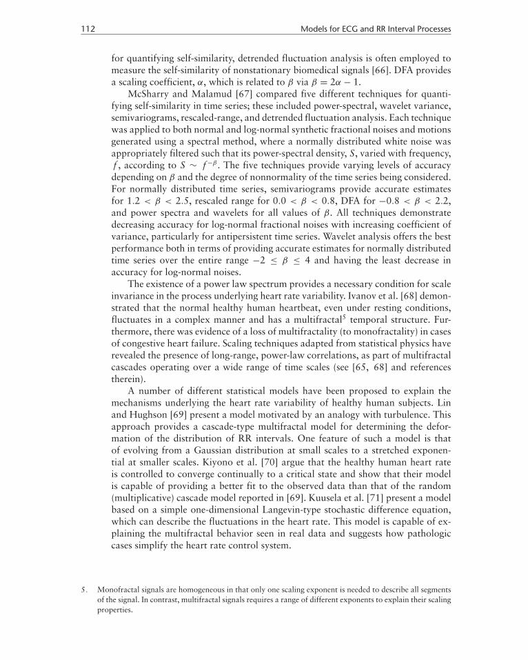
for quantifying self-similarity, detrended fluctuation analysis is often employed tomeasure the self-similarity of nonstationary biomedical signals [66]. DFA providesa scaling coefficient, α, which is related to β via β = 2α − 1.

McSharry and Malamud [67] compared five different techniques for quanti-fying self-similarity in time series; these included power-spectral, wavelet variance,semivariograms, rescaled-range, and detrended fluctuation analysis. Each techniquewas applied to both normal and log-normal synthetic fractional noises and motionsgenerated using a spectral method, where a normally distributed white noise wasappropriately filtered such that its power-spectral density, S, varied with frequency,f , according to S ∼ f −β . The five techniques provide varying levels of accuracydepending on β and the degree of nonnormality of the time series being considered.For normally distributed time series, semivariograms provide accurate estimatesfor 1.2 < β < 2.5, rescaled range for 0.0 < β < 0.8, DFA for −0.8 < β < 2.2,and power spectra and wavelets for all values of β. All techniques demonstratedecreasing accuracy for log-normal fractional noises with increasing coefficient ofvariance, particularly for antipersistent time series. Wavelet analysis offers the bestperformance both in terms of providing accurate estimates for normally distributedtime series over the entire range −2 ≤ β ≤ 4 and having the least decrease inaccuracy for log-normal noises.

The existence of a power law spectrum provides a necessary condition for scaleinvariance in the process underlying heart rate variability. Ivanov et al. [68] demon-strated that the normal healthy human heartbeat, even under resting conditions,fluctuates in a complex manner and has a multifractal5 temporal structure. Fur-thermore, there was evidence of a loss of multifractality (to monofractality) in casesof congestive heart failure. Scaling techniques adapted from statistical physics haverevealed the presence of long-range, power-law correlations, as part of multifractalcascades operating over a wide range of time scales (see [65, 68] and referencestherein).

A number of different statistical models have been proposed to explain themechanisms underlying the heart rate variability of healthy human subjects. Linand Hughson [69] present a model motivated by an analogy with turbulence. Thisapproach provides a cascade-type multifractal model for determining the defor-mation of the distribution of RR intervals. One feature of such a model is thatof evolving from a Gaussian distribution at small scales to a stretched exponen-tial at smaller scales. Kiyono et al. [70] argue that the healthy human heart rateis controlled to converge continually to a critical state and show that their modelis capable of providing a better fit to the observed data than that of the random(multiplicative) cascade model reported in [69]. Kuusela et al. [71] present a modelbased on a simple one-dimensional Langevin-type stochastic difference equation,which can describe the fluctuations in the heart rate. This model is capable of ex-plaining the multifractal behavior seen in real data and suggests how pathologiccases simplify the heart rate control system.

5. Monofractal signals are homogeneous in that only one scaling exponent is needed to describe all segmentsof the signal. In contrast, multifractal signals requires a range of different exponents to explain their scalingproperties.

P1: Shashi



4.2.8 PhysioNet Challenge

The PhysioNet challenge of 20026 invited participants to design a numerical modelfor generating 24-hour records of RR intervals. A second part of the challengeasked participants to use their respective signal processing techniques to identifythe real and artificial records from among a database of unmarked 24-hour RRtachograms. The wide range of models entered for the competition reflects the nu-merous approaches available for investigating heart rate variability. The followingparagraphs summarize these approaches, which include a multiplicative cascademodel, a Markovian model, and a heuristic multiscale approach based on empiricalobservations.

Lin and Hughson [69] explored the multifractal HRV displayed in healthyand other physiological conditions, including autonomic blockades and congestiveheart failure, by using a multiplicative random cascade model. Their method useda bounded cascade model to generate artificial time series which was able to mimicsome of the known phenomenology of HRV in healthy humans: (1) multifractalspectrum including 1/ f power law, (2) the transition from stretch-exponential toGaussian probability density function in the interbeat interval increment data and(3) the Poisson excursion law in small RR increments [72]. The cascade consistedof a discrete fragmentation process and assigned random weights to the cascadecomponents of the fragmented time intervals. The artificial time series was finallyconstructed by multiplying the cascade components in each level.

Yang et al. [73] employed symbolic dynamics and probabilistic automaton toconstruct a Markovian model for characterizing the complex dynamics of healthyhuman heart rate signals. Their approach was to simplify the dynamics by mappingthe output to binary sequences, where the increase and decrease of the interbeatinterval were denoted by 1 and 0, respectively. In this way, it was also possible todefine a m-bit symbolic sequence to characterize transitions of symbolic dynamics.For the simplest model consisting of 2-bit sequences, there are four possible sym-bolic sequences including 11, 10, 00, and 01. Moreover, each symbolic sequencehas two possible transitions, for example, 1(0) can be transformed to (0)0, whichresults in decreasing RR intervals, or (0)1 and vice versa. In order to define themechanism underlying these symbolic transitions, the authors utilized the conceptof probabilistic automaton in which the transition from current symbolic sequenceto next state takes place with a certain probability in a given range of RR intervals.The model used 8-bit sequences and a probability table obtained from the RR timeseries of healthy humans from Taipei Veterans General Hospital and PhysioNet.The resulting generator is comprised of the following major components: (1) thesymbolic sequence as a state of RR dynamics, (2) the probability table definingtransitions between two sequences, and (3) an absolute Gaussian noise process forgoverning increments of RR intervals.

McSharry et al. [74] used a heuristic empirical approach for modeling thefluctuations of the beat-to-beat RR intervals of a normal healthy human over24 hours by considering the different time scales independently. Short range vari-ability due to Mayer waves and RSA were incorporated into the algorithm using a

6. See http://www.physionet.org/challenge/2002 for more details.

P1: Shashi



power spectrum with given spectral characteristics described by its low frequencyand high frequency components, respectively [75]. Longer range fluctuations aris-ing from transitions between physiological states were generated using switchingdistributions extracted from real data. The model generated realistic synthetic 24-hour RR tachograms by including both cardiovascular interactions and transitionsbetween physiological states. The algorithm included the effects of various physi-ological states, including sleep states, using RR intervals with specific means andtrends. An analysis of ectopic beat and artifact incidence in an accompanying pa-per [76] was used to provide a mechanism for generating realistic ectopy and artifact.Ectopic beats were added with an independent probability of one per hour. Artifactswere included with a probability proportional to mean heart rate within a state andincreased for state transition periods. The algorithm provides RR tachograms thatare similar to those in the MIT-BIH Normal Sinus Rhythm Database.

4.2.9 RR Interval Models for Abnormal Rhythms

Chapter 1 described some of the mechanisms that activate and mediate arrhythmiasof the heart. Broadly speaking, modeling of arrhythmias can be broken down intotwo subgroups: ventricular arrhythmias and atrial arrhythmias. The models tendto describe either the underlying RR interval processes or the manifest waveform(ECG). Furthermore, the models are formulated either from the cellular conductionperspective (usually for RR interval models) or from an empirical standpoint. Sincethe connection between the underlying beat-to-beat interval process and the resul-tant waveform is complex, empirical models of the ECG waveform are common.These include simple time domain templates [77], Fourier and AR models [78],singular value decomposition-based techniques [79, 80], and more complex meth-ods such as neural network classifiers [81–83], and finite element models [84]. Suchmodels are usually applied on a beat-by-beat basis. Furthermore, due to the fact thatthe classifiers are trained using a cost function based upon a distance metric betweenwaveforms, small deviations in the waveform morphology (such as that seen in atrialarrhythmias) are often poorly identified. In the case of atrial arrhythmias, unlessa full three-dimensional model of the cardiac potentials is used (such as in Cherryet al. [85]), it is often more appropriate to analyze the RR interval process itself.

The following gives a chronological summary of the developments in modelingatrial fibrillation. In 1983, Cohen et al. [86] introduced a model for the ventricularresponse during AF that treated the atrio-ventricular junction as a lumped parameterstructure with defined electrical properties such as the refactory period and periodof autorhymicity, that is being continually bombarded by random AF impulses.Although this model could account for all the principal statistical properties of theRR interval distribution during AF, several important physiological properties ofthe heart were not included in the model (such as conduction delays within the AVjunction and ventricle and the effect of ventricular pacing).

In 1988, Wittkampf et al. [87–89] explained the fact that short RR intervalsduring AF could be eliminated by ventricular pacing at relatively long cycle lengthsthrough a model that modulates the AV node pacemaker rate and rhythm by AFimpulses. However, this model failed to explain the relationship between most ofthe captured beats and the shortest RR interval length in a canine model.

P1: Shashi


4.3 ECG Models 115

In 1996, Meijler et al. [90] proposed an alternative model whereby the irreg-ularity of RR intervals during AF are explained by modulation of the AV nodethrough concealed AF impulses resulting in an inverse relationship between theatrial and ventricular rates. Unfortunately, recent clinical results do not support thisprediction.

Around the same time Zeng and Glass [91] introduced an alternative modelof AV node conduction which was able to correctly model much of the statisticaldistribution of the RR intervals during AF. This model was later extended by Tatenoand Glass [92] and Jorgensen et al. [93] and includes a description of the AV delaytime, τ AVD, (which is known to be dependent on the AV junction recovery time)given by

τ AVD = τ AVDmin + αe−TR/c (4.6)

where TR is the AV junction recovery time, τ AVDmin is the minimum AV delay when

TR → ∞, α is the maximum extension of the AV delay when TR = 0, and c is a timeconstant. Although this extension modeled many of the properties of AF, it failedto account for the dependence of the refactory period, τ R, on the heart rate (thehigher the heart rate, the shorter the refactory period) [86].

Lian et al. [94] recently proposed an extension of Cohen’s model [86] whichdoes model the refactory behavior of the AV junction as

τ AVJ = τ AVJmin + τ AVJ

ext (1 − e−TR/τext ) (4.7)

where τ AVJmin is the shortest AV junction refactory period corresponding to TR = 0

and τ AVJext is the maximum extension of the refactory period when TR → ∞. The AV

delay (4.6) is also included in this model together with a function which expresses themodulation of the AV junction refactory period by blocked impulses. If an impulseis blocked by the refactory AV junction, τ AVJ is prolonged by the concealed impulsesuch that

τ AVJ → τ AVJ + τ AVJmin

(t

τ AVJ

)θ [max

(1,

�V(VT − VR)

)]δ

(4.8)

where �V/(VT −VR) is the relative amplitude of the AF pulses and t (0 < t < τ AVJ )is the time when the impulse is blocked. θ and δ are independent parameters whichmodulate the timing and duration of the blocked impulse. With suitably chosenvalues for the above parameters, this model can account for all the statistical prop-erties of observed RR intervals processes during AF (see Lian et al. [94] for furtherdetails and experimental results).

4.3 ECG Models

The following sections show two disparate approaches to modeling the ECG. Whileboth paradigms can produce an ECG signal and are consistent with various as-pects of the physiology, they attempt to replicate different observed phenomena on

P1: Shashi



different temporal scales. Section 4.3.1 presents the first approach, based on com-putational physiology, which employs first principles to derive the fundamentalequations and then integrates this information using a three-dimensional anatomi-cal description of the heart. This approach, although complex and computationallyintensive, often provides a model which furthers our understanding of the effects ofsmall changes or defects in cardiac physiology. Section 4.3.2 describes the secondapproach which appeals to an empirical description of the ECG, whereby statisticalquantities such as the temporal and spectral characteristics of both the ECG andassociated heart rate are modeled. Given that these quantities are routinely used forclinical diagnosis, this latter approach is of interest in the field of biomedical signalprocessing.

4.3.1 Computational Physiology

While the ECG is routinely used to diagnose arrhythmias, it reflects an integratedsignal and cannot provide information on the micro-spatial scales of cells and ionicchannels. For this reason, the field of computational cardiac modeling and simu-lation has grown over the last decade. In the following, we consider a variety ofapproaches to whole heart modeling.

The fundamental approach to whole heart modeling is based on the finite ele-ment method, which partitions the entire heart and chest into numerous elementswhere each element represents a group of cells. The ECG may then be simulated bycalculating the body surface potential of each cardiac element [95]. This approach,however, fails to relate the ECG waveform with the micro-scale cellular electrophys-iology. The use of membrane equations is needed to incorporate the mechanisms atcell, channel, and molecular level [96]. In the following, we review some promis-ing research in the area of whole heart modeling, such as cellular autonoma andmultiscale modeling approaches.

Arrhythmias are often initiated by abnormal electrical activity at the cellularscale or the ionic channel level. Cellular automata provide an effective means ofconstructing whole heart models and of simulating such arrhythmias, which maydisplay a spatio-temporal evolution within the heart [97]. Such models combine adifferential description of electrical properties of cardiac cells using membrane equa-tions. This approach relates the ECG waveform to the underlying cellular activityand is capable of describing a range of pathological conditions. Cluster computingis employed as a means of dealing with the necessary computationally intensivesimulations.

A single autonoma cell may be viewed as a computing unit for the action po-tential and ECG simulation. The electrical activity of these cells is described bycorresponding Hodgkin-Huxley action potential equations. Zhu et al. [97] con-structed a three-dimensional heart model based on data from the axial images ofthe Visible Human Project digital male cadaver [98]. The anatomical model of theheart utilized a data file to describe the distribution of the cell array and the char-acteristics of each cell.

Understanding the complexity of the heart requires biological models of cells,tissues, organs, and organ systems. The present aim is to combine the bottom-up approach of investigating interactions at the lower spatial scales of proteins

P1: Shashi


4.3 ECG Models 117

(receptors, transporters, enzymes, and so forth) with that of the top-down approachof modeling organs and organ systems [99]. Such a multiscale integrative approachrelies on the computational solution of physical conservation laws and anatomicallydetailed geometric models [100].

Multiscale models are now possible because of three recent developments:(1) molecular and biophysical data on many proteins and genes is now available(e.g., ion transporters [101]); (2) models exist which can describe the complexity ofbiological processes [99]; and (3) continuing improvements in computing resourcesallow the simulation of complex cell models with hundreds of different proteinfunctions on a single-processor computer whereas parallel computers can now dealwith whole organ models [102].

The interplay between simulation and experimentation has given rise to modelsof sufficient accuracy for use in drug development. Numerous drugs have to bewithdrawn during trials due to cardiac side effects that are usually associated withirregular heartbeats and abnormal ECG morphologies. Noble and Rudy [103] haveconstructed a model of the heart that is able to provide an accurate description atthe cellular level. Simulations of this model have been of great value to improvingthe understanding of the complex interactions underlying the heart. Furthermore,such computer-based heart models, known as in silico screening, provide a meansof simulating and understanding the effects of drugs on the cardiovascular system.In particular these models can now be used to investigate the regulation of drugtherapy.

While the grand challenge of heart modeling is to simulate a full-scale coronaryheart attack, this would require extensive computing power [99]. Another hindranceis the lack of transfer of both data and models between different research centers.In addition, there is no standard representation for these models, thereby limitingthe communication of innovative ideas and decreasing the pace of research. Oncethese hurdles have been overcome, the eventual aim is the development of integratedmodels comprising cells, organs, and organ systems.

4.3.2 Synthetic Electrocardiogram Signals

When only a realistic ECG is required (such as in the testing of signal processingalgorithms), we may use an alternative approach to modeling the heart. ECGSYNis a dynamical model for generating synthetic ECG signals with arbitrary mor-phologies (i.e., any lead configuration) where the user has the flexibility to choosethe operating characteristics. The model was motivated by the need to evaluateand quantify the performance of the signal processing techniques on ECG signalswith known characteristics. An early attempt to produce a synthetic ECG gener-ator [104] (available from the PhysioNet Web site [30] along with ECGSYN) isnot intended to be highly realistic, and includes no P wave, and no variations intiming or morphology and discontinuities. In contrast to this, ECGSYN is basedupon time-varying differential equations and is continuous with convincing beat-to-beat variations in morphology and interbeat timing. ECGSYN may be employedto generate extremely realistic ECG signals with complete flexibility over the choiceof parameters that govern the structure of these ECG signals in both the temporaland spectral domains. The model also allows the average morphology of the ECG

P1: Shashi



Figure 4.4 ECGSYN flow chart describing the procedure for specifying the temporal and spectraldescription of the RR tachogram and ECG morphology.

to be fully specified. In this way, it is possible to simulate ECG signals that showsigns of various pathological conditions.

Open-source code in Matlab and C and further details of the model may beobtained from the PhysioNet Web site.7 In addition a Java applet may be utilisedin order to select model parameters from a graphical user interface, allowing theuser to simulate and download an ECG signal with known characteristics. Theunderlying algorithm consists of two parts. The first stage involves the generation ofan internal time series with internal sampling frequency fint to incorporate a specificmean heart rate, standard deviation and spectral characteristics corresponding toa real RR tachogram. The second stage produces the average morphology of theECG by specifying the locations and heights of the peaks that occur during eachheartbeat. A flow chart of the various processes in ECGSYN for simulating theECG is shown in Figure 4.4.

Spectral characteristics of the RR tachogram, including both RSA and Mayerwaves, are replicated by describing a bimodal spectrum composed of the sum of

7. See http://www.physionet.org/physiotools/ecgsyn/.

P1: Shashi


4.3 ECG Models 119

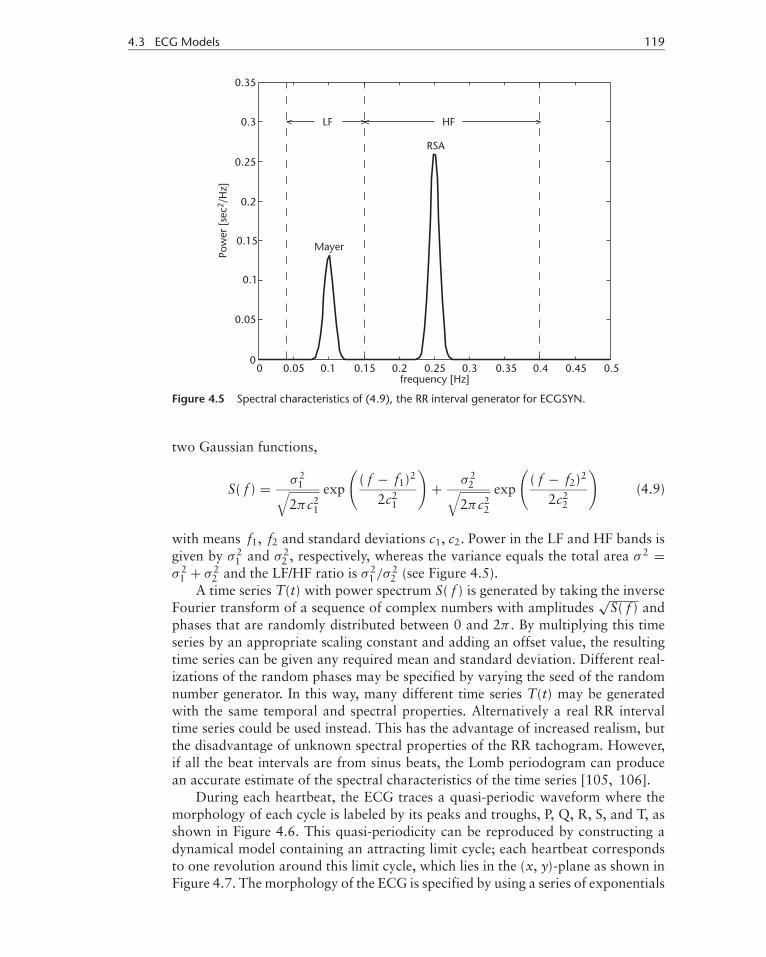
Figure 4.5 Spectral characteristics of (4.9), the RR interval generator for ECGSYN.

two Gaussian functions,

S( f ) = σ 21√

2πc21

exp

(( f − f1)2

2c21

)+ σ 2

2√2πc2

2

exp

(( f − f2)2

2c22

)(4.9)

with means f1, f2 and standard deviations c1, c2. Power in the LF and HF bands isgiven by σ 2

1 and σ 22 , respectively, whereas the variance equals the total area σ 2 =

σ 21 + σ 2

2 and the LF/HF ratio is σ 21 /σ 2

2 (see Figure 4.5).A time series T(t) with power spectrum S( f ) is generated by taking the inverse

Fourier transform of a sequence of complex numbers with amplitudes√

S( f ) andphases that are randomly distributed between 0 and 2π . By multiplying this timeseries by an appropriate scaling constant and adding an offset value, the resultingtime series can be given any required mean and standard deviation. Different real-izations of the random phases may be specified by varying the seed of the randomnumber generator. In this way, many different time series T(t) may be generatedwith the same temporal and spectral properties. Alternatively a real RR intervaltime series could be used instead. This has the advantage of increased realism, butthe disadvantage of unknown spectral properties of the RR tachogram. However,if all the beat intervals are from sinus beats, the Lomb periodogram can producean accurate estimate of the spectral characteristics of the time series [105, 106].

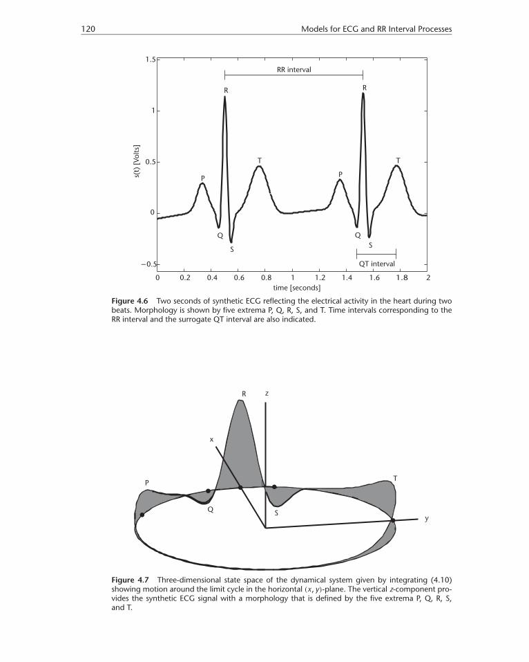
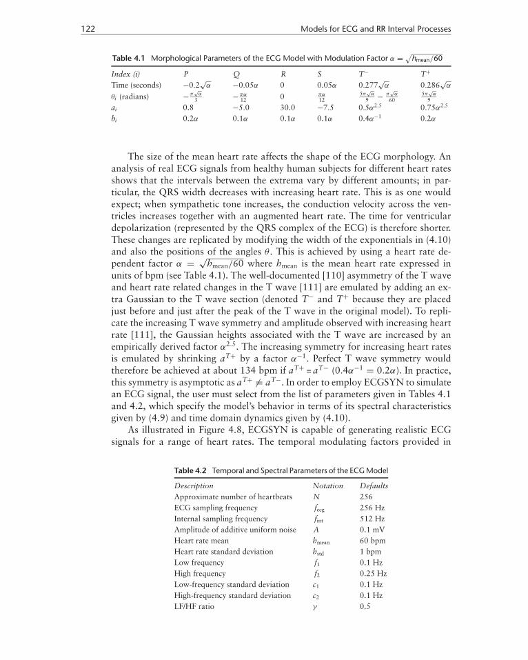
During each heartbeat, the ECG traces a quasi-periodic waveform where themorphology of each cycle is labeled by its peaks and troughs, P, Q, R, S, and T, asshown in Figure 4.6. This quasi-periodicity can be reproduced by constructing adynamical model containing an attracting limit cycle; each heartbeat correspondsto one revolution around this limit cycle, which lies in the (x, y)-plane as shown inFigure 4.7. The morphology of the ECG is specified by using a series of exponentials

P1: Shashi



Figure 4.6 Two seconds of synthetic ECG reflecting the electrical activity in the heart during twobeats. Morphology is shown by five extrema P, Q, R, S, and T. Time intervals corresponding to theRR interval and the surrogate QT interval are also indicated.

Figure 4.7 Three-dimensional state space of the dynamical system given by integrating (4.10)showing motion around the limit cycle in the horizontal (x, y)-plane. The vertical z-component pro-vides the synthetic ECG signal with a morphology that is defined by the five extrema P, Q, R, S,and T.

P1: Shashi


4.3 ECG Models 121

to force the trajectory to trace out the PQRST-waveform in the z-direction. A seriesof five angles, (θP , θQ, θR, θS, θT), describes the extrema of the peaks (P, Q, R, S, T),respectively.

The dynamical equations of motion are given by three ordinary differentialequations [107],

x = αx − ωy

y = αy + ωx

z = −∑

i∈{P,Q,R,S,T−,T+}ai�θi exp(−�θ2

i /2b2i ) − (z − z0) (4.10)

where α = 1 −√x2 + y2, �θi = (θ − θi ) mod 2π , θ = atan2(y, x) and ω is the

angular velocity of the trajectory as it moves around the limit cycle. The coefficientsai govern the magnitude of the peaks whereas the bi define the width (time duration)of each peak. Note that the T wave is often asymmetrical and therefore requirestwo Gaussians, T− and T+ (rather than one), to correctly model this asymmetry(see [108]). Baseline wander may be introduced by coupling the baseline value z0

in (4.10) to the respiratory frequency f2 in (4.9) using z0(t) = Asin(2π f2t). Theoutput synthetic ECG signal, s(t), is the vertical component of the three-dimensionaldynamical system in (4.10): s(t) = z(t).

Having calculated the internal RR tachogram expressed by the time series T(t)with power spectrum S( f ) given by (4.9), this can then be used to drive the dy-namical model (4.10) so that the resulting RR intervals will have the same powerspectrum as that given by S( f ). Starting from the auxiliary8 time tn, with angleθ = θR, the time interval T(tn) is used to calculate an angular frequency �n = 2π

T(tn) .This particular angular frequency, �n, is used to specify the dynamics until the an-gle θ reaches θR again, whereby a complete revolution (one heartbeat) has takenplace. For the next revolution, the time is updated, tn+1 = tn + T(tn), and the nextangular frequency, �n+1 = 2π

T(tn+1) , is used to drive the trajectory around the limitcycle. In this way, the internally generated beat-to-beat time series, T(t), can beused to generate an ECG signal with associated RR intervals that have the samespectral characteristics. The angular frequency ω(t) in (4.10) is specified using thebeat-to-beat values �n obtained from the internally generated RR tachogram:

ω(t) = �n, tn ≤ t < tn+1 (4.11)

A fourth-order Runge-Kutta method [109] is used to integrate the equationsof motion in (4.10) using the beat-to-beat values of the angular frequency �. Thetime series T(t) used for defining the values of �n has a high sampling frequency offint, which is effectively the step size of the integration. The final output ECG signalis then downsampled to fecg if fint > fecg by a factor of fint

fecgin order to generate

an ECG signal at the requested sampling frequency. In practice fint is taken as aninteger multiple of fecg for simplicity.

8. This auxiliary time axis is used to calculate the values of �n for consecutive RR intervals, whereas the timeaxis for the ECG signal is sampled around the limit cycle in the (x, y)-plane.

P1: Shashi



Table 4.1 Morphological Parameters of the ECG Model with Modulation Factor α = √hmean/60

Index (i) P Q R S T− T+

Time (seconds) −0.2√

α −0.05α 0 0.05α 0.277√

α 0.286√

α

θi (radians) − π√

α

3 − πα12 0 πα

125π

√α

9 − π√

α

605π

√α

9

ai 0.8 −5.0 30.0 −7.5 0.5α2.5 0.75α2.5

bi 0.2α 0.1α 0.1α 0.1α 0.4α−1 0.2α

The size of the mean heart rate affects the shape of the ECG morphology. Ananalysis of real ECG signals from healthy human subjects for different heart ratesshows that the intervals between the extrema vary by different amounts; in par-ticular, the QRS width decreases with increasing heart rate. This is as one wouldexpect; when sympathetic tone increases, the conduction velocity across the ven-tricles increases together with an augmented heart rate. The time for ventriculardepolarization (represented by the QRS complex of the ECG) is therefore shorter.These changes are replicated by modifying the width of the exponentials in (4.10)and also the positions of the angles θ . This is achieved by using a heart rate de-pendent factor α = √

hmean/60 where hmean is the mean heart rate expressed inunits of bpm (see Table 4.1). The well-documented [110] asymmetry of the T waveand heart rate related changes in the T wave [111] are emulated by adding an ex-tra Gaussian to the T wave section (denoted T− and T+ because they are placedjust before and just after the peak of the T wave in the original model). To repli-cate the increasing T wave symmetry and amplitude observed with increasing heartrate [111], the Gaussian heights associated with the T wave are increased by anempirically derived factor α2.5. The increasing symmetry for increasing heart ratesis emulated by shrinking aT+ by a factor α−1. Perfect T wave symmetry wouldtherefore be achieved at about 134 bpm if aT+ = aT− (0.4α−1 = 0.2α). In practice,this symmetry is asymptotic as aT+ �= aT−. In order to employ ECGSYN to simulatean ECG signal, the user must select from the list of parameters given in Tables 4.1and 4.2, which specify the model’s behavior in terms of its spectral characteristicsgiven by (4.9) and time domain dynamics given by (4.10).

As illustrated in Figure 4.8, ECGSYN is capable of generating realistic ECGsignals for a range of heart rates. The temporal modulating factors provided in

Table 4.2 Temporal and Spectral Parameters of the ECG Model

Description Notation DefaultsApproximate number of heartbeats N 256ECG sampling frequency fecg 256 HzInternal sampling frequency fint 512 HzAmplitude of additive uniform noise A 0.1 mVHeart rate mean hmean 60 bpmHeart rate standard deviation hstd 1 bpmLow frequency f1 0.1 HzHigh frequency f2 0.25 HzLow-frequency standard deviation c1 0.1 HzHigh-frequency standard deviation c2 0.1 HzLF/HF ratio γ 0.5

P1: Shashi


4.3 ECG Models 123

Figure 4.8 Synthetic ECG signals for different mean heart rates: (a) 30 bpm, (b) 60 bpm, and(c) 120 bpm.

Table 4.1 ensure that the various intervals, such as the PR, QT, and QRS, decreasewith increasing heart rate. A nonlinear relationship between the morphology mod-ulation factor α and the mean heart rate hmean decreases the temporal contraction ofthe overall PQRST morphology with respect to the refractory period (the minimumamount of time in which depolarization and repolarization of the cardiac musclecan occur). This is consistent with the changes in parasympathetic stimulation con-nected to changes in heart rate; a higher heart rate due to sympathetic stimulationleads to an increase in conduction velocity across the ventricles and an associatedreduction in QRS width. Note that the changes in angular frequency, ω, around thelimit cycle, resulting from the period changes in each RR interval, do not lead totemporal changes, but to amplitude changes. For example, decreases in RR interval(higher heart rates) will not only lead to less broad QRS complexes, but also tolower amplitude R peaks, since the limit cycle will have less time to reach the max-imum value of the Gaussian contribution given by aR, bR, and θR. This realistic(parasympathetically mediated) amplitude variation [112, 113], which is due torespiration-induced mechanical changes in the heart position with respect to theelectrode positions in real recordings, is dominated by the high-frequency com-ponent in (4.9), which reflects parasympathetic activity in our model. This phe-nomenon is independent of the respiratory-coupled baseline wander in this modelwhich is coupled to the peak HF frequency in a rather ad hoc manner. Of course,this part of the model could be made more realistic by coupling the baseline wanderto a phase-lagged signal derived from highpass filtering (fc = 0.15 Hz) the RR

P1: Shashi



interval time series. The phase lag is important, since RSA and mechanical effectson the ECG and RR time series are not in phase (and often drift based on a sub-ject’s activity [3]). The beat-to-beat changes in RR intervals in this model faithfullyreproduce RSA effects (decreases in RR interval with inspiration and increases withexpiration) for lead configurations taken in the sense of lead I. Therefore, althoughthe morphologies in the figures are modeled after lead II or V5, the amplitude mod-ulation of the R peaks acts in the opposite sense to that which is seen on real lead IIor V5 electrode configurations. That is, on inspiration (expiration) the amplitudeof the model-derived R peaks decrease (increase) rather than increase (decrease).This is a reflection of the fact that these changes are a mechanical artifact on realECG recordings, rather than a direct result of the neural mediated mechanisms.(A recent addition to the model, proposed by Amann et al. [114], includes anamplitude modulation term in z in (4.10) and may be used to provide the requiredmodulation in such cases.) Furthermore, the phase lag between the RSA effect andthe R peak modulation effect is fixed, reflecting the fact that this model is assum-ing a stationary state for each instance of generation. Extensions to this model, tocouple it to a 24-hour RR time series, were presented in [115], where the entiresequence was composed of a series of RR tachograms, each having a stationarystate with different characteristics reflecting observed normal circadian changes(see [74] and Section 4.2.8).

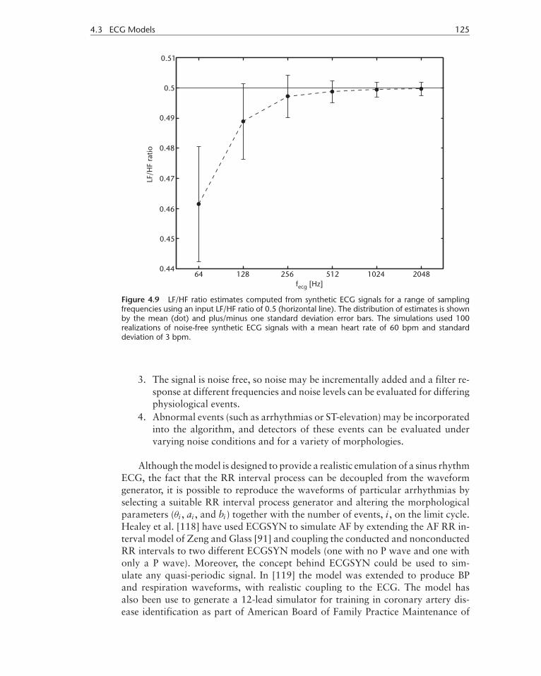
ECGSYN can be employed to generate ECG signals with known spectral char-acteristics and can be used to test the effect of varying the ECG sampling fre-quency fecg on the estimation of HRV metrics. In the following analysis, estimatesof the LF/HF ratio were calculated for a range of sampling frequencies (Figure 4.9).ECGSYN was operated using a mean heart rate of 60 bpm, a standard deviation of3 bpm, and a LF/HF ratio of 0.5. Error bars representing one standard deviationon either side of the means (dots) using a total of 100 Monte Carlo runs are alsoshown.

The LF/HF ratio was estimated using the Lomb periodogram. As this tech-nique introduces negligible variance into the estimate [105, 106, 116], it may beconcluded that the underestimation of the LF/HF ratio is due to the sampling fre-quency being too small. The analysis indicates that the LF/HF ratio is considerablyunderestimated for sampling frequencies below 512 Hz. This result is consistentwith previous investigations performed on real ECG signals [61, 106, 117]. In ad-dition, it provides a guide for clinicians when selecting the sampling frequency ofthe ECG based on the required accuracy of the HRV metrics.

The key features of ECGSYN which make this type of model such a useful toolfor testing signal processing algorithms are as follows:

1. A user can rapidly generate many possible morphologies at a range of heartrates and HRVs (determined separately by the standard deviation and theLF/HF ratio). An algorithm can therefore be tested on a vast range of ECGs(some of which can be extremely rare and therefore underrepresented indatabases).

2. The sampling frequency can be varied and the response of an algorithm canbe evaluated.

P1: Shashi


4.3 ECG Models 125

Figure 4.9 LF/HF ratio estimates computed from synthetic ECG signals for a range of samplingfrequencies using an input LF/HF ratio of 0.5 (horizontal line). The distribution of estimates is shownby the mean (dot) and plus/minus one standard deviation error bars. The simulations used 100realizations of noise-free synthetic ECG signals with a mean heart rate of 60 bpm and standarddeviation of 3 bpm.

3. The signal is noise free, so noise may be incrementally added and a filter re-sponse at different frequencies and noise levels can be evaluated for differingphysiological events.

4. Abnormal events (such as arrhythmias or ST-elevation) may be incorporatedinto the algorithm, and detectors of these events can be evaluated undervarying noise conditions and for a variety of morphologies.

Although the model is designed to provide a realistic emulation of a sinus rhythmECG, the fact that the RR interval process can be decoupled from the waveformgenerator, it is possible to reproduce the waveforms of particular arrhythmias byselecting a suitable RR interval process generator and altering the morphologicalparameters (θi , ai , and bi ) together with the number of events, i , on the limit cycle.Healey et al. [118] have used ECGSYN to simulate AF by extending the AF RR in-terval model of Zeng and Glass [91] and coupling the conducted and nonconductedRR intervals to two different ECGSYN models (one with no P wave and one withonly a P wave). Moreover, the concept behind ECGSYN could be used to sim-ulate any quasi-periodic signal. In [119] the model was extended to produce BPand respiration waveforms, with realistic coupling to the ECG. The model hasalso been use to generate a 12-lead simulator for training in coronary artery dis-ease identification as part of American Board of Family Practice Maintenance of

P1: Shashi



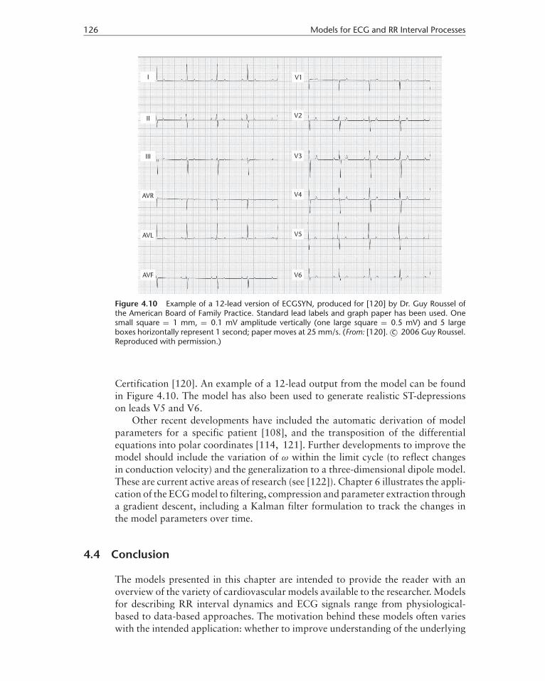
Figure 4.10 Example of a 12-lead version of ECGSYN, produced for [120] by Dr. Guy Roussel ofthe American Board of Family Practice. Standard lead labels and graph paper has been used. Onesmall square = 1 mm, = 0.1 mV amplitude vertically (one large square = 0.5 mV) and 5 largeboxes horizontally represent 1 second; paper moves at 25 mm/s. (From: [120]. c© 2006 Guy Roussel.Reproduced with permission.)

Certification [120]. An example of a 12-lead output from the model can be foundin Figure 4.10. The model has also been used to generate realistic ST-depressionson leads V5 and V6.

Other recent developments have included the automatic derivation of modelparameters for a specific patient [108], and the transposition of the differentialequations into polar coordinates [114, 121]. Further developments to improve themodel should include the variation of ω within the limit cycle (to reflect changesin conduction velocity) and the generalization to a three-dimensional dipole model.These are current active areas of research (see [122]). Chapter 6 illustrates the appli-cation of the ECG model to filtering, compression and parameter extraction througha gradient descent, including a Kalman filter formulation to track the changes inthe model parameters over time.

4.4 Conclusion

The models presented in this chapter are intended to provide the reader with anoverview of the variety of cardiovascular models available to the researcher. Modelsfor describing RR interval dynamics and ECG signals range from physiological-based to data-based approaches. The motivation behind these models often varieswith the intended application: whether to improve understanding of the underlying

P1: Shashi


4.4 Conclusion 127

control mechanisms or to attempt to obtain a better fit to the observed biomedicalsignals.

Applications of these models have included model fitting [29, 108], compres-sion and filtering [119, 123], and classification [124]. However, the required com-plexity for realistic models (particularly for ECG generation) has limited the devel-opment of using model parameters for classifying hemodynamic and cardiac states.The assumed increase in computing power and utilization of parallel processingis likely to stimulate research in these fields in the near future. Simplified (andtractable) models such as ECGSYN provide a realistic current alternative. Chapter6 describes a model fitting procedure that can run on a beat-by-beat basis in realtime on a modern desktop computer.

Computational physiology is now at the stage where it is possible to integratemodels from the level of the cell to that of the organ. By taking a multidisciplinaryapproach to systems biology, the ability to construct in silico models that reflect theunderlying physiology and match the observed signals has the potential to deliverconsiderable advances in the field of biomedical science.

References

[1] Hales, S., Statical Essays II, Haemastaticks, London, U.K.: Innings and Manby, 1733.[2] Ludwig, C., “Beitrage zur Kenntnis des Einflusses der Respirationsbewegung auf den

Blutlauf im Aortensystem,” Arch. Anat. Physiol., Vol. 13, 1847, pp. 242–302.[3] Hoyer, D., et al., “Validating Phase Relations Between Cardiac and Breathing Cycles

During Sleep,” IEEE Eng. Med. Biol., March/April 2001.[4] Thomas, R. J., et al., “An Electrocardiogram-Based Technique to Assess Cardiopul-

monary Coupling During Sleep,” Sleep, Vol. 28, No. 9, October 2005, pp. 1151–1161.

[5] DeBoer, R. W., J. M. Karemaker, and J. Strackee, “Hemodynamic Fluctuations andBaroreflex Sensitivity in Humans: A Beat-to-Beat Model,” Am. J. Physiol., Vol. 253,1987, pp. 680–689.

[6] Malik, M., “Heart Rate Variability: Standards of Measurement, Physiological Interpre-tation, and Clinical Use,” Circulation, Vol. 93, 1996, pp. 1043–1065.

[7] Sleight, P., and B. Casadei, “Relationships Between Heart Rate, Respiration and BloodPressure Variabilities,” in M. Malik and A. J. Camm, (eds.), Heart Rate Variability,Armonk, NY: Futura Publishing, 1995, pp. 311–327.

[8] Ottesen, J. T., “Modeling of the Baroreflex-Feedback Mechanism with Time-Delay,”J. Math. Biol., Vol. 36, 1997, pp. 41–63.

[9] Ottesen, J. T., M. S. Olufsen, and J. K. Larsen, Applied Mathematical Models in Hu-man Physiology, Philadelphia, PA: SIAM Monographs on Mathematical Modeling andComputation, 2004.

[10] Grodins, F. S., “Integrative Cardiovascular Physiology: A Mathematical Synthesis ofCardiac and Blood Pressure Vessel Hemodynamics,” Q. Rev. Biol., Vol. 34, 1959,pp. 93–116.

[11] Madwed, J. B., et al., “Low Frequency Oscillations in Arterial Pressure and HeartRate: A Simple Computer Model,” Am. J. Physiol., Vol. 256, 1989, pp. H1573–H1579.

[12] Ursino, M., M. Antonucci, and E. Belardinelli, “Role of Active Changes in Venous Ca-pacity by the Carotid Beroreflex: Analysis with a Mathematical Model,” Am. J. Physiol.,Vol. 267, 1994, pp. H2531–H2546.

P1: Shashi



[13] Ursino, M., A. Fiorenzi, and E. Belardinelli, “The Role of Pressure Pulsatility in theCarotid Baroreflex Control: A Computer Simulation Study,” Comput. Bio. Med., Vol. 26,No. 4, 1996, pp. 297–314.

[14] Ursino, M., “Interaction Between Carotid Baroregulation and the Pulsating Heart: AMathematical Moodel,” Am. J. Physiol., Vol. 275, 1998, pp. H1733–H1747.

[15] Seidel, H., and H. Herzel, “Bifurcations in a Nonlinear Model of the Baroreceptor Car-diac Reflex,” Physica D, Vol. 115, 1998, pp. 145–160.

[16] McSharry, P. E., M. J. McGuinness, and A. C. Fowler, “Comparing a CardiovascularSystem Model with Heart Rate and Blood Pressure Data,” Computers in Cardiology,Vol. 32, September 2005, pp. 587–590.

[17] Baselli, G., S. Cerutti, and S. Civardi, “Cardiovascular Variability Signals: Toward theIdentification of a Closed-Loop Model of the Neural Control Mechanisms,” IEEE Trans.Biomed. Eng., Vol. 35, 1988, pp. 1033–1046.

[18] Saul, J. P., R. D. Berger, and P. Albrecht, “Transfer Function Analysis of the Circulation:Unique Insights into Cardiovascular Regulation,” Am. J. Physiol. (Heart Circ. Physiol.),Vol. 261, No. 4, 1991, pp. H1231–H1245.

[19] Batzel, J., and F. Kappel, “Survey of Research in Modeling the Human Respiratory andCardiovascular Systems,” in R. C. Smith and M. A. Demetriou, (eds.), Research Direc-tions in Distributed Parameter Systems, SIAM Series: Frontiers in Applied Mathematics,Philadelphia, PA: SIAM, 2003.

[20] Whittam, A. M., et al., “Computer Modeling of Heart Rate and Blood Pressure,” Com-puters in Cardiology, Vol. 25, 1998, pp. 149–152.

[21] Pitzalis, M. V., et al., “Effect of Respiratory Rate on the Relationship Between π In-terval and Systolic Blood Pressure Fluctuations: A Frequency-Dependent Phenomenon,”Cardiovascular Research, Vol. 38, 1998, pp. 332–339.

[22] Mukkamala, R., and R. J. Cohen, “A Cardiovascular Simulator for Research,”http://www.physionet.org/physiotools/rcvsim/.

[23] Mukkamala, R., and R. J. Cohen, “A Forward Model-Based Validation of CardiovascularSystem Identification,” Am. J. Physiol.: Heart Circ. Physiol., Vol. 281, No. 6, 2001,pp. H2714–H2730.

[24] Mukkamala, R., K. Toska, and R. J. Cohen, “Noninvasive Identification of the TotalPeripheral Resistance Baroreflex,” Am. J. Physiol., Vol. 284, No. 3, 2003, pp. H947–H959.

[25] Peng, C. K., et al., “Long-Range Anticorrelations and Non-Gaussian Behavior of theHeartbeat,” Physical Review Letters, Vol. 70, No. 9, 1993, pp. 1343–1346.

[26] Heldt, E. B., et al., “Computational Modeling of Cardiovascular Responses to Or-thostatic Stress,” Journal of Applied Physiology, Vol. 92, 2002, pp. 1239–1254,http://mimic.mit.edu/Archive/Papers/heldtpaper2.pdf.

[27] Heldt, T., and R. G. Mark, “Scaling Cardiovascular Parameters for Population Simula-tion,” Computers in Cardiology, IEEE Computer Society Press, Vol. 31, September 2004,pp. 133–136, http://mimic.mit.edu/Archive/Papers/heldtpaper2.pdf.

[28] Heldt, T., “Orthostatic Hypotension,” Ph.D. dissertation, Massachusetts Institute ofTechnology, 2005.

[29] Samar, Z., “Parameter Fitting of a Cardiovascular Model,” M.S. thesis, MassachusettsInstitute of Technology, 2005.

[30] Goldberger, A. L., et al., “Physiobank, Physiotoolkit, and Physionet: Components ofa New Research Resource for Complex Physiologic Signals,” Circulation, Vol. 101,No. 23, 2000, pp. e215–e220.

[31] Rompelman, O., A. J. R. M. Coenen, and R. I. Kitney, “Measurement of Heart-RateVariability—Part 1: Comparative Study of Heart-Rate Variability Analysis Methods,”Med. Biol. Eng. & Comput., Vol. 15, 1977, pp. 239–252.

P1: Shashi


4.4 Conclusion 129

[32] Mateo, J., and P. Laguna, “Improved Heart Rate Variability Signal Analysis from theBeat Occurrence Times According to the IPFM Model,” IEEE Trans. Biomed. Eng., Vol.47, No. 8, 2000, pp. 985–996.

[33] Rompelman, O., J. D. Snijders, and C. van Spronsen, “The Measurement of Heart RateVariability Spectra with the Help of a Personal Computer,” IEEE Trans. Biomed. Eng.,Vol. 29, 1982, pp. 503–510.

[34] Hyndman, B. W., and R. K. Mohn, “A Model of the Cardiac Pacemaker and Its Usein Decoding the Information Content of Cardiac Intervals,” Automedia, Vol. 1, 1975,pp. 239–252.

[35] Seydnejad, S. R., and R. I. Kitney, “Time-Varying Threshold Integral Pulse FrequencyModulation,” IEEE Trans. Biomed. Eng., Vol. 48, No. 9, 2001, pp. 949–962.

[36] Kantz, H., and T. Schreiber, Nonlinear Time Series Analysis, Cambridge, U.K.: Cam-bridge University Press, 1997.

[37] Theiler, J., et al., “Testing for Nonlinearity in Time Series: The Method of SurrogateData,” Physica D, Vol. 58, 1992, pp. 77–94.

[38] Farmer, J. D., and J. J. Sidorowich, “Predicting Chaotic Time Series,” Phys. Rev. Lett.,Vol. 59, No. 8, 1987, pp. 845–848.

[39] Casdagli, M., “Nonlinear Prediction of Chaotic Time Series,” Physica D, Vol. 35, 1989,pp. 335–356.

[40] Smith, L. A., “Identification and Prediction of Low-Dimensional Dynamics,” Physica D,Vol. 58, 1992, pp. 50–76.

[41] Broomhead, D. S., and D. Lowe, “Multivariable Functional Interpolation and AdaptiveNetworks,” J. Complex Systems, Vol. 2, 1988, pp. 321–355.

[42] Bishop, C., Neural Networks for Pattern Recognition, New York: Oxford UniversityPress, 1995.

[43] McSharry, P. E., and L. A. Smith, “Consistent Nonlinear Dynamics: Identifying ModelInadequacy,” Physica D, Vol. 192, 2004, pp. 1–22.

[44] Cao, L., and A. Mees, “Deterministic Structure in Multichannel Physiological Data,”International Journal of Bifurcation and Chaos, Vol. 10, No. 12, 2000, pp. 2767–2780.

[45] Weigend, A. S., and N. A. Gershenfeld, Time Series Prediction: Forecasting the Future andUnderstanding the Past, Volume 15, SFI Studies in Complexity, Reading, MA: Addison-Wesley, 1993.

[46] Petrillo, G. A., L. Glass, and T. Trippenbach, “Phase Locking of the Respiratory Rhythmin Cats to a Mechanical Ventilator,” Canadian Journal of Physiology and Pharmacology,Vol. 61, 1983, pp. 599–607.

[47] Bracic Lotric, A., and M. Stefanovska, “Synchronization and Modulation in the HumanCardiorespiratory System,” Physica A, Vol. 283, 2000, p. 451.

[48] Rosenblum, M. G., et al., “Synchronization in Noisy Systems and CardiorespiratoryInteraction,” IEEE Eng. Med. Biol. Mag., Vol. 17, No. 6, November–December 1998,pp. 46–53.

[49] Schafer, C., et al., “Heartbeat Synchronization with Ventilation,” Nature, Vol. 392,March 1998, pp. 239–240.

[50] Toledo, E., et al., “Quantification of Cardiorespiratory Synchronization in Normal andHeart Transplant Subject,” Proc. of Int. Symposium on Nonlinear Theory an Applica-tions (NOLTA), Vol. 1, Presses Polytechnique et Universitaires Romandes, September1998, pp. 171–174.

[51] Toledo, E., et al., “Cardiorespiratory Synchronization: Is It a Real Phenomenon?” inA. Murray and S. Swiryn, (eds.), Computers in Cardiology, Hannover, Germany: IEEEComputer Society, Vol. 26, 1999, pp. 237–240.

P1: Shashi



[52] Stefanovska, A., et al., “The Cardiovascular System as Coupled Oscillators?” Physiol.Meas., Vol. 22, 2001, pp. 535–550.

[53] Stefanovska, A., D. G. Luchinsky, and V. E. McClintock, “Modeling Couplings Amongthe Oscillators of the Cardiovascular System,” Physiol. Meas., Vol. 22, 2001, pp. 551–564.

[54] Ichimaru, Y., et al., “Effect of Sleep Stage on the Relationship Between Respiration andHeart Rate Variability,” Computers in Cordiology, Vol. 17, 1990, pp. 657–660.

[55] Lavie, P., A. Schlitner, and R. Nave, “Cardiac Automatic Function During Sleep inPsychogenic and Organic Erectile Dysfunction,” J. Sleep Res., Vol. 8, 1999, pp. 135–142.

[56] Otzenberger, H., et al., “Dynamic Heart Rate Variability: A Tool for Exploring Sym-pathovagal Balance Continuously During Sleep in Men,” Am. J. Physiol.: Heart Circ.Physiol., Vol. 275, 1998, pp. H946–H950.

[57] Ivanov, P. C., et al., “Sleep Wake Differences in Scaling Behavior of the Human Heartbeat:Analysis of Terrestrial and Long-Term Space Flight Data,” Europhys. Lett., Vol. 48,No. 5, 1999, pp. 594–600.

[58] Bunde, A., et al., “Correlated and Uncorrelated Regions in Heart-Rate FluctuationsDuring Sleep,” Phy. Rev. Lett., Vol. 85, No. 17, October 2000.

[59] Ferini-Strambi, L., et al., “The Impact of Cyclic Alternating Pattern on Heart-Rate Vari-ability During Sleep in Healthy Young Adults,” Clinical Neurophysiology, Vol. 111,No. 1, January 2000, pp. 99–101.

[60] Ferri, R., et al., “Cyclic Alternating Pattern and Spectral Analysis of Heart Rate Vari-ability During Normal Sleep,” J. Sleep Res., Vol. 9, 2000, pp. 13–18.

[61] Clifford, G. D., and L. Tarassenko, “Segmenting Cardiac-Related Data Using Sleep StagesIncreases Separation Between Normal Subjects and Apnoeic Patients,” IOP Physiol.Means., 2004.

[62] Lo, C. -C., et al., “Common Scale-Invariant Patterns of Sleep-Wake Transitions AcrossMammalian Species,” PNAS, Vol. 101, No. 50, 2004, pp. 17545–17548.

[63] Kobayashi, M., and T. Musha, “1/f Fluctuation of Heartbeat Period,” IEEE Trans.Biomed. Eng., Vol. 29, 1982, p. 456.

[64] Theorie de l’Addition des Variables Aleatoires, Paris, France: Gauthier Villars, 1937.[65] Goldberger, A. L., et al., “Fractal Dynamics in Physiology: Alterations with Disease and

Ageing,” Proc. Natl. Acad. Sci., Vol. 99, 2002, pp. 2466–2472.[66] Peng, C. -K., et al., “Quantification of Scaling Exponents and Crossover Phenomena in

Nonstationary Heartbeat Time Series,” Chaos, Vol. 5, 1995, pp. 82–87.[67] McSharry, P. E., and B. D. Malamud, “Quantifying Self-Similarity in Cardiac Inter-Beat

Interval Time Series,” Computers in Cardiology, Vol. 32, September 2005, pp. 462–495.[68] Ivanov, P. C., et al., “Multifractality in Human Heartbeat Dynamics,” Nature, Vol. 399,

1999, pp. 461–465.[69] Lin, D. C., and R. L. Hughson, “Modeling Heart Rate Variability in Healthy Humans:

A Turbulence Analogy,” Phys. Rev. Lett., Vol. 86, No. 8, 2001, pp. 1650–1653.[70] Kiyono, K., et al., “Critical Scale Invariance in a Healthy Human Heart Rate,” Phys.

Rev. Lett., Vol. 93, No. 17, 2004, pp. 178103–17.[71] Kuusela, T., “Stochastic Heart-Rate Model Can Reveal Pathologic Cardiac Dynamics,”

Phys. Rev. E, Vol. 69, 2004, p. 031916.[72] Lin, D. C., and J. Thevaril, “Simulate Heart Rate Variability in Different Physiological

Conditions,” Computers in Cardiology, Vol. 29, 2002, pp. 149–152.[73] Yang, C. C., et al., “Simulating Healthy Humans Heart Rate: A Model Using Symbolic

Dynamics and Probabilistic Automaton,” Computers in Cardiology, Vol. 29, 2002, pp.229–232.

P1: Shashi


4.4 Conclusion 131

[74] McSharry, P. E., et al., “Method for Generating an Artificial RR Tachogram of a TypicalHealthy Human over 24-Hours,” Computers in Cardiology, Vol. 29, September 2002,pp. 225–228.

[75] McSharry, P. E., et al., “A Dynamical Model for Generating Synthetic ElectrocardiogramSignals,” IEEE Trans. Biomed. Eng., Vol. 50, No. 3, 2003, pp. 289–294.

[76] Clifford, G., P. E. McSharry, and L. Tarassenko, “Characterizing Artifact in the Nor-mal Human 24-Hour RR Time Series to Aid Identification and Artificial Replication ofCircadian Variations in Human Beat to Beat Heart Rate Using a Simple Threshold,”Computers in Cardiology, Vol. 29, September 2002, pp. 129–132.

[77] Medilog Manual, Old Woking: Oxford Medical Instruments.[78] Dingfei, G., N. Srinivasan, and S. Krishnan, “Cardiac Arrhythmia Classification Using

Autoregressive Modeling,” BioMedical Engineering OnLine, Vol. 1, No. 1, 2002, p. 5.[79] Moody, G. B., and R. G. Mark, “QRS Morphology Representation and Noise Estima-

tion Using the Karhunen-Loeve Transform,” Computers in Cardiology, Vol. 16, 1989,pp. 269–272.

[80] Mark, R. G., and G. B. Moody, “ECG Arrhythmia Analysis: Design and EvaluationStrategies,” Chapter 18, in I. Gath and G. F. Inbar, (eds.), Advances in Processing andPattern Analysis of Biological Signals, New York: Plenum Press, 1996, pp. 251–272.

[81] Clifford, G. D., L. Tarassenko, and N. Townsend, “Fusing Conventional ECG QRS De-tection Algorithms with an Auto-Associative Neural Network for the Detection of Ec-topic Beats,” 5th International Conference on Signal Processing, Beijing, China, August2000, IFIP, World Computer Congress, pp. 1623–1628.

[82] Tarassenko, L., G. D. Clifford, and N. Townsend, “Detection of Ectopic Beats in the Elec-trocardiogram Using an Auto-Associative Neural Network,” Neural Processing Letters,Vol. 14, No. 1, 2001, pp. 15–25.

[83] Clifford, G. D., and L. Tarassenko, “One-Pass Training of Optimal Architecture Auto-Associative Neural Network for Detecting Ectopic Beats,” IEE Electronic Letters,Vol. 37, No. 18, August 2001, pp. 1126–1127.

[84] Hastings, H., et al., “Alternans and the Onset of Ventricular Fibrillation,” Physical Re-view E, 2000, pp. 4043–4048.

[85] Cherry, E. M., et al., “The Role of Decreased Conduction Velocity in the Initiation andMaintenance of Atrial Fibrillation in a Computer Model of Human Atria,” Pacing andClinical Electrophysiology, Part II, 2002, p. 538.

[86] Cohen, R. J., R. D. Berger, and T. E. Dushane, “A Quantative Model for the VentricularEscape Response During Atrial Fibrillation,” IEEE Trans. Biomed. Eng., 1983, pp. 769–781.

[87] Wittkampf, F. H., et al., “Effect of Right Ventricular Pacing on Ventricular RhythmDuring a Atrial Fibrillation,” J. Am. Coll. Cardiol., 1988, pp. 539–545.

[88] Wittkampf, F. H., M. J. L. DeJongste, and F. L. Meijler, “Atrioventricular Nodal Responseto Retrograde Action in Atrial Fibrillation,” J. Cardiovascular Electro-Physiology, 1990,pp. 437–447.

[89] Wittkampf, F. H., M. J. L. DeJongste, and F. L. Meijler, “Competitive Antegrade and Ret-rograde Atrioventricular Junctional Activation in Atrial Fibrillation,” J. CardiovascularElectrophysiology, 1990, pp. 448–456.

[90] Meijler, F. L., et al., “AV Nodal Function During Atrial Fibrillation: The Role of ElectronicModulation of Propagation,” J. Cardiovascular Electrophysiology, 1996, pp. 843–861.

[91] Zeng, W., and L. Glass, “Statistical Properties of Heartbeat Intervals During Atrial Fib-rillation,” Phys. Rev. E, 1996, pp. 1779–1784.

[92] Glass, L., and K. Tateno, “Automatic Detection of Atrial Fibrillation Using the Coefficientof Variation and Density Histograms of RR and DRR Intervals,” Medical and BiologicalEngineering and Computing, 2001, pp. 664–671.

P1: Shashi



[93] Jorgensen, P., et al., “A Mathematical Model of Human Atrioventricular Nodal Func-tion Incorporating Concealed Conduction,” Bulletin of Mathematical Biology, 2002,pp. 1083–1099.

[94] Lian, J., D. Mussig, and V. Lang, “Computer Modeling of Ventricular Rhythm DuringAtrial Fibrillation and Ventricular Pacing,” IEEE Trans. Biomed. Eng., Vol. 53, No. 8,2006, pp. 1512–1520.

[95] Shahidi, A. V., and P. Savard, “Forward Problem of Electrocardiography: Constructionof Human Torso Models and Field Calculations Using Finite Element Method,” Med.Biol. Eng. Comput., Vol. 32, 1994, pp. S25–S33.

[96] Thakor, N. V., et al., “Electrophysiologic Models of Heart Cells and Cell Networks,”IEEE Engineering in Medicine and Biology, Vol. 17, No. 5, 1998, pp. 73–83.

[97] Zhu, H., et al., “Facilitating Arrhythmia Simulation: The Method of Quantitative Cellu-lar Automata Modeling and Parallel Running,” BioMedical Engineering OnLine, Vol. 3,2004, p. 29.

[98] Ackerman, M. J., “The Visible Human Project: A Resource for Anatomical Visualiza-tion,” Medinfo, Vol. 9, 1998, pp. 1030–1032.

[99] Noble, D., “Modeling the Heart: From Genes to Cells to the Whole Organ,” Science,Vol. 295, 2002, pp. 1678–1682.

[100] Crampin, E. J., et al., “Computational Physiology and the Physiome Project,” Experi-mental Physiology, Vol. 89, No. 1, 2004, pp. 1–26.

[101] Ashcroft, F. M., Ion Channels and Disease, San Diego, CA: Academic Press, 2000.[102] Kohl, P., et al., “Computational Modeling of Biological Systems: Tools and Visions,”

Phil. Trans. Roy. Soc. A, Vol. 358, 2000, pp. 579–610.[103] Noble, D., and Y. Rudy, “Models of Cardiac Ventricular Action Potentials: Iterative

Interaction Between Experiment and Simulation,” Phil. Trans. R. Soc. A, Vol. 359, 2001,pp. 1127–1142.

[104] Ruha, A., and S. Nissila, “A Real-Time Microprocessor QRS Detector System with a1-ms Timing Accuracy for the Measurement of Ambulatory HRV,” IEEE Trans. Biomed.Eng., Vol. 44, No. 3, 1997, pp. 159–167.

[105] Laguna, P., G. B. Moody, and R. G. Mark, “Power Spectral Density of Unevenly SampledData by Least-Square Analysis: Performance and Application to Heart Rate Signals,”IEEE Trans. Biomed. Eng, Vol. BME-45, 1998, pp. 698–715.

[106] Clifford, G. D., and L. Tarassenko, “Quantifying Errors in Spectral Estimates of HRVDue to Beat Replacement and Resampling,” IEEE Trans. Biomed. Eng., Vol. 52, No. 4,April 2005.

[107] McSharry, P. E., et al., “A Dynamical Model for Generating Synthetic ElectrocardiogramSignals,” IEEE Trans. Biomed. Eng., Vol. 50, No. 3, 2003, pp. 289–294.

[108] Clifford, G. D., et al., “Model-Based Filtering, Compression and Classification of theECG,” Joint Meeting of 5th International Conference on Bioelectromagnetism and 5thInternational Symposium on Noninvasive Functional Source Imaging within the HumanBrain and Heart (BEM & NFSI), Minnesota, May 2005, invited paper.

[109] Press, W. H., et al., Numerical Recipes in C, 2nd ed., Cambridge, U.K.: CambridgeUniversity Press, 1992.

[110] Zareba, W., and A. J. Moss, “Dispersion of Repolarization; Relation to Heart Rate andRepolarization Duration,” J. Electrocardiol., No. 28, 1995, pp. 202–206.

[111] di Bernardo, D., P. Langley, and A. Murray, “Effect of Changes in Heart Rate and inAction Potential Duration on the Electrocardiogram T Wave Shape,” Physiological Mea-surement, Vol. 23, No. 2, 2002, pp. 355–364.

[112] Moody, G. B., et al., “Derivation of Respiratory Signals from Multi-Lead ECGs,” Com-puters in Cardiology, Vol. 12, 1985, pp. 113–116.

[113] Moody, G. B., et al., “Clinical Validation of the ECG-Derived Respiration (EDR) Tech-nique,” Computers in Cardiology, Vol. 13, 1986, pp. 507–510.

P1: Shashi


4.4 Conclusion 133

[114] Amann, A., and K. Klotz, “Improved Models for Generating Synthetic ElectrocardiogramSignals,” IEEE Trans. Biomed. Eng., 2005, in submission.

[115] Clifford, G. D., and P. E. McSharry, “Generating 24-Hour ECG, BP and RespiratorySignals with Realistic Linear and Nonlinear Clinical Characteristics Using a NonlinearModel,” Computers in Cardiology, Vol. 31, 2004, pp. 709–712.

[116] Clifford, G. D., “Signal Processing Methods for Heart Rate Variability,” Ph.D. disserta-tion, University of Oxford, 2002.

[117] Abboud, S., and O. Barnea, “Errors Due to Sampling Frequency of Electrocardiogram inSpectral Analysis of Heart Rate Signals with Low Variability,” Computers in Cardiology,Vol. 22, September 1995, pp. 461–463.

[118] Healey, J., et al., “An Open-Source Method for Simulating Atrial Fibrillation UsingECGSYN,” Computers in Cardiology, Vol. 31, No. 19–22, September 2004, pp. 425–428.

[119] Clifford, G. D., and P. E. McSharry, “A Realistic Coupled Nonlinear Artificial ECG,BP, and Respiratory Signal Generator for Assessing Noise Performance of BiomedicalSignal Processing Algorithms,” Proc of SPIE International Symposium on Fluctuationsand Noise, Vol. 5467, No. 34, 2004, pp. 290–301.

[120] Roussel, G., “Coronary Artery Disease Simulation,” American Board ofFamily Medicine Maintenance of Certification for Family Physicians, 2006,https://www.theabfm.org/moc/.

[121] Sameni, R., M. B. Shamsollahi, and C. Jutten, “Filtering Noisy Signals Using theExtended Kalman Filter Based on a Modified Dynamic ECG Model,” Computers inCardiology, Vol. 32, September 2005, pp. 5639–5642.

[122] Sameni, R., et al., “A Nonlinear Bayesian Filtering Framework for ECG Denoising,”submitted to IEEE Trans. Biomed. Eng., 2005.

[123] McSharry, P. E., and G. D. Clifford, “A Comparison of Nonlinear Noise Reductionand Independent Component Analysis Using a Realistic Dynamical Model of theElectrocardiogram,” Proc. of SPIE International Symposium on Fluctuations andNoise, Vol. 5467, No. 9, 2004, pp. 78–88.

[124] Heldt, T., et al., “Computational Model of Cardiovascular Function During OrthostaticStress,” Computers in Cardiology, Vol. 27, 2000, pp. 777–780.

CHAPTER 4 Models for ECG and RR Interval Processesgari/ecgbook/ch4.pdfP1: Shashi August 24, 2006...

Documents

Transcript of CHAPTER 4 Models for ECG and RR Interval Processesgari/ecgbook/ch4.pdfP1: Shashi August 24, 2006...