Chapter 4 Conﬁdence Intervals in Ridge Regression using Jackknife and Bootstrap...

Chapter 4

Confidence Intervals in Ridge

Regression using Jackknife and

Bootstrap Methods

4.1 Introduction

It is now explicable that ridge regression estimator (here we take ordinary ridge

estimator (ORE) in particular) can be of great use for estimating the unknown

regression coefficients in the presence of multicollinearity. But apart from its

ability to create good parameter estimates with smaller MSE than the OLSE,

it must also provide fine solutions when dealing with more intricate inference

problems like obtaining confidence intervals. The problem with the ORE is

that its sampling distribution is unknown, hence we make use of the resampling

methods to obtain the asymptotic confidence intervals for the regression coef-

ficients based on the ORE. Recently, Firinguetti and Bobadilla [40] developed

asymptotic confidence intervals for the regression coefficients based on ORE and

Edgeworth expansion. Crivelli et. al. [17] proposed the use of a technique that

combines the bootstrap and the Edgeworth expansion to obtain an approxima-

tion to the distribution of some ridge regression estimators and carried out some

simulation experiments. Alheety and Ramanathan [4] proposed a data depen-

dent confidence interval for the ridge parameter k.

Confidence intervals have become very popular in the applied statistician’s col-

73

CHAPTER 4. CONFIDENCE INTERVALS IN RIDGE REGRESSIONUSING JACKKNIFE AND BOOTSTRAP METHODS

lection of data-analytic tools. They combine point estimation and hypothesis

testing into a single inferential statement. Recent advances in statistical meth-

ods and fast computing allow the construction of highly accurate approximate

confidence intervals. Confidence intervals for a given population parameter θ are

sample based range [θ1, θ2] given out for the unknown θ. The range possesses the

property that θ would lie within its bounds with a high specified probability. Of

course this probability is with respect to all possible samples, each sample giving

rise to a confidence interval which depends on the chance mechanism involved

in drawing the samples. Two approaches for confidence intervals includes the

construction of exact intervals for special cases like the ratio of normal means or

a single binomial parameter and others are the most commonly used, approxi-

mate confidence intervals which are also known as standard intervals (or normal

theory intervals) having the following form

θ ± z(α)σ, (4.1.1)

where θ is a point estimate of the parameter θ, σ is an estimate of standard de-

viation of θ, and z(α) is the 100αth percentile of a normal variate, (for example

z(0.95) = 1.645 etc.). The main drawback of standard intervals is that they are

based on an asymptotic approximation that may not be accurate in practice.

There has been considerable progress on developing better confidence intervals

techniques for improving the standard interval, involving bias corrections and

parameter transformations etc.. Numerous methods have been proposed to im-

prove upon standard intervals. These methods produce approximate confidence

intervals that have better coverage accuracy than the standard one. Some ref-

erences under this area includes McCullagh [67], Cox and Reid [16], Efron [34],

Hall [49], DiCiccio and Tibshirani [24] etc.. The confidence intervals based on

the resampling methods like bootstrap and jackknife can be seen as automatic

algorithms for carrying out these improvements. We have already discussed that

bootstrap and jackknife are two powerful methods for variance estimation which

is why we can use them to produce confidence intervals. We discuss the different

methods for construction of the bootstrap and jackknife confidence intervals in

Section (4.2) and (4.3) respectively, Section (4.4) contains the model and the

estimators, Section (4.5) gives a simulation study for the comparison of cover-

age probabilities and average confidence widths based on ORE and OLSE and

Ph.D. Thesis: Mansi Khurana

74


Section (4.6) consists of some concluding remarks.

4.2 Bootstrap Confidence Intervals

Suppose that we draw a sample S = (x1, x2, ...., xn) of size n from a popula-

tion of size N and we are interested in some statistic θ as an estimate of the

corresponding population parameter θ. The classical inference, where we de-

rive the asymptotic distribution of sampling distribution of θ when its exact

distribution is intractable or has some drawbacks. The corresponding sampling

distribution of statistic θ may be inaccurate if the assumptions about the pop-

ulation are wrong or the sample size is relatively small. On the other hand,

as discussed earlier also, nonparametric bootstrap enables us to estimate the

sampling distribution of a statistic empirically without making any assump-

tions about the parent population and without deriving sampling distribution

explicitly. In this method, we draw a sample of size n from the elements of

sample S and the sampling is done with replacement. This is the first bootstrap

resample S∗

1 = (x∗

11, x∗

12, ...., x∗

1n). Each element of the resample is selected from

the original sample with probability 1/n. We repeat this step of resampling

a large number of times say B so that the rth bootstrap resample is given by

S∗

r = (x∗

r1, x∗

r2, ...., x∗

rn). Next, we compute the statistic θ for each of the boot-

strap resample i.e. θ∗r . Now, the distribution of θ∗r around the original statistic

θ is similar to the sampling distribution of θ around population parameter θ.

The average of the statistics computed based on bootstrap resamples estimates

the expectation of the bootstrapped statistic. It is given as

¯θ∗ =

∑Br=1 θ∗rB

.

Then B∗ =¯θ∗ − θ gives an estimate of bias of θ which is θ − θ. The estimate of

the bootstrap variance of θ∗ is

V (θ∗) =

∑Br=1(θ

∗

r −¯θ∗)2

B − 1,

which estimates the sampling variance of θ. With the help of this variance es-

timate, we can easily produce bootstrap confidence intervals. There are several


75


methods for constructing bootstrap confidence intervals, each of them are briefly

discussed below.

4.2.1 Normal Theory Method

The first method for constructing bootstrap confidence interval is based on the

assumption that the sampling distribution of θ is normal. This uses the boot-

strap estimate of sampling variance to construct a 100(1 − α)% confidence in-

terval of the following form

(2θ − ¯θ∗) ± z(1−α/2)SE(θ∗),

where SE(θ∗) =

√

V (θ∗) is the bootstrap estimate of the standard error of θ

and z(1−α/2) is the (1 − α/2) quantile of the standard normal distribution.

4.2.2 Bootstrap Percentile and Centered Bootstrap Per-

centile Method

Another method for the construction of bootstrap confidence intervals is the

bootstrap percentile method which is the most popular among all primarily

due to its simplicity and natural appeal. In this method, we use the empirical

quantiles of θ∗ to form the confidence interval for θ. The bootstrap percentile

confidence interval has the following form

θ∗(lower) < θ < θ∗(upper),

where θ∗(1), θ∗

(2), ..., θ∗

(B) are the ordered bootstrap replicates of θ with lower con-

fidence limit=[(B + 1)α/2] and upper confidence limit=[(B + 1)(1−α/2)]. The

square brackets indicates rounding to the nearest integer. For example, there are

1000 bootstrap replications (i.e. B = 1000) for θ, denoted by (θ∗1, θ∗

2, ..., θ∗

1000).

After sorting them from bottom to top, let us denote these bootstrap values as

(θ∗(1), θ∗

(2), ..., θ∗

(1000)). Then the bootstrap percentile confidence interval at 95%

level would be [θ∗(25), θ∗

(975)]. Here, it is implicitly assumed that the distribution


76


of θ is symmetric around θ as the method approximates the sampling distribu-

tion of (θ− θ) by the bootstrap distribution of (θ− θ∗) which is contrary to the

bootstrap theory. The coverage error is substantial if the distribution of θ is not

nearly symmetric.

Now, suppose the sampling distribution of (θ− θ) is approximated by the boot-

strap distribution of (θ∗ − θ) which is what bootstrap theory explains. Then

the statement that (θ − θ) lies within the range(B0.025 − θ, B0.975 − θ) would

carry a probability of 0.95 where Bs denotes the 100sth percentile of bootstrap

distribution of θ∗. In case of 1000 bootstrap replications B0.025 = θ∗(25) and

B0.975 = θ∗(975), we see that the above statement reduces to the statement that θ

lies in the following confidence interval

(2θ − B0.975) < θ < (2θ − B0.025).

The above mentioned range is known as centered bootstrap percentile confi-

dence interval. This method can be applied to any statistic and works well in

cases where the bootstrap distribution is symmetrical and centered around the

observed statistic.

4.2.3 Bootstrap Studentized-t Method

Another method for constructing the bootstrap confidence intervals is the stu-

dentized bootstrap, also called the bootstrap-t method. The studentized-t boot-

strap confidence interval takes the same form as the normal confidence interval

except that instead of using the quantiles from a normal distribution, a boot-

strapped t-distribution is constructed from which the quantiles are computed

(see Davison and Hinkley [21] and Efron and Tibshirani [35]). Bootstrapping a

statistical function of the form t = (θ − θ)/(SE), where SE is the sample esti-

mate of the standard error of θ brings extra accuracy. This additional accuracy

is due to the so called one-term Edgeworth correction by the bootstrap (see Hall

[50]). The basic example of it is the standard t− statistics t = (x− µ)/(s/√

n),

which is a special case with θ = µ (the population mean), θ = x (the sample

mean) and s being the sample standard deviation. The bootstrap counterpart


77


of this is

t∗ = (θ∗ − θ)/(SE)∗,

where SE∗ is the standard error based on bootstrap distribution. Denote the

100sth bootstrap percentile of t∗ by bs and consider the statement that (b0.025 <

t < b0.975) and after substituting t = (θ − θ)/SE, we get confidence limits for θ

as

θ − (SE)b0.975 < θ < θ − (SE)b0.025.

This range is known as bootstrap-t based confidence interval for θ at 95% con-

fidence level. Like the normal approximation, this confidence interval leads to

interval estimates that are symmetric about the original point estimator, which

may not be appropriate. It is best suited for bootstrapping a location statistic.

The use of the studentized bootstrap is controversial to some extent. In some

cases, the endpoints of the intervals seem to be too wide and the method seem

to be sensitive to outliers. Also, this method is computationally very intensive if

(SE)∗ is calculated using a double bootstrap but if (SE)∗ is easily available, the

method performs reliably in many examples in both its standard and variance

stabilized forms (see Davison and Hinkley [21]).

Percentile bootstrap endpoints are simple to calculate and can work well, espe-

cially if the sampling distribution is symmetrical. It may not have the correct

coverage when the sampling distribution of the statistic is skewed. Coverage of

the percentile bootstrap can be improved by adjusting the endpoints for bias

and nonconstant variance. This method is known as BCa method which we

discuss in the next subsection.

4.2.4 Bias corrected and Accelerated (BCa) Method

If we have a distribution which has skew or bias, we need to do some adjust-

ments. One method which is proved to be reliable in such cases is BCa method,

this method will tend to be closer to the true confidence interval than the per-

centile method. This is an automatic algorithm for producing highly accurate


78


confidence limits from a bootstrap distribution. For a detailed review on the

same, see Efron [34], Hall [49], DiCiccio [23], Efron and Tibshirani [35].

The BCa procedure is a method of setting approximate confidence intervals for

θ from the percentiles of the bootstrap histogram. The parameter of interest

being θ only, θ is an estimate of θ based on the observed data and θ∗ is a

bootstrap replication of θ obtained by resampling. Let G(c) be the cumulative

distribution function of B bootstrap replications of θ∗,

G(c) = #{θ∗ < c}/B. (4.2.1)

The upper endpoint, θBCa[α] of one-sided BCa interval at α level i.e. θ ∈(−∞, θBCa[α]) is defined in terms of G and two parameters z0, the bias correc-

tion and a, the acceleration. That is how BCa stands for bias corrected and

accelerated. The BCa endpoint is given by

θBCa[α] = G−1Φ

(

z0 +z0 + z(α)

1 − a(z0 + z(α))

)

. (4.2.2)

Here Φ is the standard normal c.d.f., with z(α) = Φ−1α. The central 90% BCa

confidence interval is given by (θBCa[0.05], θBCa[.95]). In (4.2.2), if a and z0 are

zero, then θBCa[α] = G−1(α), the 100αth percentile of the bootstrap replications.

Also, if G is normal, then θBCa[α] = θ + z(α)σ, the standard interval endpoint.

In general, (4.2.2) makes three different corrections to the standard intervals,

improving their coverage accuracy.

Suppose that there exists a monotone increasing transformation φ = m(θ) such

that φ = m(θ) is normally distributed for every choice of θ, but with a bias and

a non constant variance,

φ ∼ N(φ − z0σφ, σ2φ), σφ = 1 + aφ. (4.2.3)

The BCa algorithm estimates z0 by

z0 = Φ−1

{

#{θ∗(b) < θ}B

}

,

Φ−1 of the proportion of the bootstrap replications less than θ. The acceleration


79


a measures how quickly the standard error is changing on the normalized scale.

The acceleration a is estimated using the empirical influence function of the

statistic θ = t(F ),

Ui = limǫ→0t((1 − ǫ)F + ǫδi)

ǫ, i = 1, 2, . . . , n. (4.2.4)

Here δi is a point mass on xi, so (1 − ǫ)F + ǫδi is a version of F putting extra

weight on xi and less weight on the other points. The estimate of a is

a =1

6

∑ni=1 U3

i

(∑n

i=1 U2i )3/2

. (4.2.5)

There is a simpler way of calculating Ui and a. Instead of (4.2.4), we can use

the following jackknife influence function (see Hinkley [51]) in (4.2.5)

Ui = (n − 1)(θ − θ(i)), (4.2.6)

where θ(i) is the estimate of θ based on the reduced data set x(i) = (x1, x2, . . . , xi−1,

xi+1, . . . , xn).

In the next section, we discuss about the confidence intervals based on jackknife

method.

4.3 Jackknife Confidence Intervals

Jackknife technique is generally used to reduce the bias of parameter estimates

and to estimate the variance. Let n be the total sample size and the procedure

is to estimate a parameter θ for n times, each time deleting one sample data

point. The resulting estimator denoted by θ−i where the ith data point has

been excluded before calculating the estimate. The so-called pseudo values are

computed as

θi = nθ − (n − 1)θ−i,

here θ is the value of the parameter estimated from the entire data set. These

pseudo values act as independent and identical normal random variables. The

average of the above gives the jackknife estimator of θ as


80


θ =1

n

n∑

i=1

θi = nθ − (n − 1)

n

n∑

i=1

θ−i.

Also, the variance of these pseudo values is the estimate of the variance of θ

which is given by

V =1

n(n − 1)

n∑

i=1

(θi − θ)(θi − θ)′. (4.3.1)

Apart from reducing bias and estimating variance, the jackknife technique also

offers a very simple method to construct confidence interval for θ (see Miller

[71]). Now, using the consistent estimator for variance given in (4.3.1), we get

the confidence interval for θ (see Hinkley [51]) as

θ ∓ t

(

1 − α

2; n − 1

)√vii, (4.3.2)

where t

(

1 − α2; n − 1

)

is the upper α2× 100% point of the Students’s t- distri-

bution with n − 1 degrees of freedom, which is suited even for small samples.

The next section contains the model and the estimators and confidence intervals

in terms of the unknown regression coefficients.

4.4 The Model and the Estimators

Let us consider the following multiple linear regression model

y = Xβ + u (4.4.1)

where y is an (n × 1) vector of observations on the variable to be explained, X

is an (n × p) matrix of n observations on p explanatory variables assumed to

be of full column rank, β is a (p× 1) vector of regression coefficients associated

with them and u is an (n× 1) vector of disturbances, the elements of which are

assumed to be independently and identically normally distributed with

E(u) = 0; V ar(u) = σ2I.


81


The OLSE for β in model (4.4.1) is given by

βOLSE = (X ′X)−1X ′y. (4.4.2)

Now, suppose if the data has the problem of multicollinearity, we use the ORE

given by Hoerl and Kennard [52] as

βORE = (X ′X + kI)−1X ′y = (I − A−1kI)β, (4.4.3)

where k > 0 and A = X ′X + kI. The jackknife ridge estimator JRE of ORE

is calculated using the formula

βJRE = [I − (A−1kI)2]β (4.4.4)

Now for bootstrapping, firstly, for the model defined in (4.4.1), we fit the

least squares regression equation for full sample and calculate the standard-

ized residuals ui and then draw an n sized bootstrap sample with replacement

(u(b)1 , u

(b)2 , . . . , u

(b)n ) from the residuals ui’s giving 1/n probability to each ui. Af-

ter this, we obtain the bootstrap y values using the resampled residuals keeping

the design matrix fixed as shown below

y(b) = XβOLSE + u(b).

We then regress these bootstrapped y values on the fixed X to obtain the boot-

strap estimates of the regression coefficients. So, the ORE from the first boot-

strap sample is

β∗

ORE(b1) = (X ′X + kI)−1X ′y(b1).

Repeat the above steps B times where B is the number of bootstrap resamples.

Based on these, the bootstrap estimator for β is given by

¯β∗

ORE =B∑

r=1

β∗

ORE(br)/B, (4.4.5)

where r = 1, . . . , B. The estimated bias is given by

Biasest =¯β∗

ORE − βOLSE.


82


The estimated variance of ridge estimator through bootstrap is given as

V arest =B∑

r=1

(β∗

ORE(br) −¯β∗

ORE)2/(B − 1). (4.4.6)

Now, based on these estimators, we construct the confidence intervals for the

regression coefficient β in following subsection.

4.4.1 Confidence Intervals for Regression Coefficients us-

ing ORE

The different confidence intervals discussed in last section gives the following

forms for the confidence intervals in terms of the regression coefficient β.

1. Normal theory method

A 95% confidence interval for β based on ORE is

(2βORE − ¯β∗

ORE) − z(1−α/2)

√

V arest < β < (2βORE − ¯β∗

ORE) + z(1−α/2)

√

V arest,

where α = 0.05, V arest is the bootstrap estimate of the variance of βORE as

defined in (4.4.6) and z(1−α/2) is the (1 − α/2) quantile of the standard normal

distribution.

2. Percentile Method

A 95% confidence interval for 1000 bootstrap resamples would be

β∗

ORE(25) < β < β∗

ORE(975),

where β∗

ORE(r) is the rth observation in the ordered bootstrap replicates of β∗

ORE.

3. Studentized t Method

A 95% studentized t-interval would be

βORE − (SE)b0.975 < β < βORE − (SE)b0.025,


83


where bs is the 100sth bootstrap percentile of t∗ and t∗ is as defined in Section

(4.2.3).

4. BCa Method

A 95% confidence interval for β based on ORE is

βBCa[0.025] < β < βBCa[0.975],

where θBCa[α] is as defined in (4.2.2).

Another method known as the ABC (approximate bootstrap confidence inter-

vals) method has been proposed by Efron[34], that gives analytic adjustment

to BCa method for smoothly defined parameters in exponential families. They

are touted in the literature as improvements for common parametric and non-

parametric BCa procedures, and may be preferred in order to avoid the BCa’s

Monte Carlo calculations. [see avoidhese intervals are the approximations to the

BCa intervals of Efron[34], using analytic methods to avoid the BCa’s Monte

Carlo calculations [see DiCiccio and Efron [25];Efron and Tibshirani [35]; DiCi-

ccio and Efron [26]]. We have adopted this method in the linear model setup,

however we did not see significant improvement in its performance over the BCa

method. Hence, this method is not pursued in the numerical investigations car-

ried out later.

5. Jackknife Method

A 95% jackknife confidence interval for β based on ORE is

βJRE − t

(

1 − α

2; n − p

)√vii < β < βJRE + t

(

1 − α

2; n − p

)√vii, (4.4.7)

where α = 0.05, t

(

1− α2; n− p

)

is the upper α2× 100% point of the Students’s

t-distribution with (n− p) degrees of freedom and vii is as given in (4.3.1) with

(n − 1) in the denominator being replaced by (n − p).

In order to compare these methods of constructing asymptotic confidence inter-


84


vals based on ORE and OLSE, we calculate coverage probabilities which is de-

fined as the proportion that the confidence interval includes the true parameter,

under repeated sampling from the same underlying population and confidence

width which is the difference between the upper and lower confidence endpoints.

In the next section, we carry out a simulation study to obtain the confidence

widths and coverage probabilities based on the confidence intervals developed

using ORE and OLSE.

4.5 A Simulation Study

After getting into some theoretical aspects of each method to construct confi-

dence intervals, we now apply the methods on simulated data and compare the

performance ORE and OLSE based on their coverage probabilities and confi-

dence widths. The model is

y = Xβ + u (4.5.1)

where u ∼ N(0, 1). Here β is taken as the normalized eigen vector corresponding

to the largest eigen value of X ′X. The explanatory variables are generated from

the following equation

xij = (1 − ρ2)1

2 wij + ρwip, i = 1, 2. . . . , n; j = 1, 2, . . . , p.

where wij are independent standard normal pseudo-random numbers and ρ2 is

the correlation between xij and xij′ for j, j′ < p and j 6= j′. When j or j′ = p,

the correlation will be ρ. We have taken ρ = 0.9 and 0.99 to investigate the

effects of different degrees of collinearity with sample sizes n = 25, 50 and 100.

The feasible value of k is obtained by the optimal formula k = pσ2

β′βas given by

Hoerl et al. [53], so that

k =pσ2

β′β,

where

σ2 =(y − Xβ)′(y − Xβ)

n − p.


85


For calculating different bootstrap confidence intervals like Normal, Percentile,

Studentized and BCa, we have used the function called ‘boot.ci’ in R. The

confidence limits through jackknife are calculated using (4.4.7) and variance

of jackknifed estimator is calculated using bootstrap method for variance esti-

mation. We have calculated the coverage probabilities and average confidence

width using 1999 bootstrap resamples and the experiment is repeated 500 times.

The coverage probability, say CP is calculated using the following formula

CP =#(βL < β < βU)

N,

and the average confidence width, say CW is calculated by

CW =

∑Ni=1(βU − βL)

N,

where N is the simulation size, βL and βU are lower and upper confidence in-

terval endpoints respectively. The results for coverage probability and average

confidence width at 95% and 99% confidence levels with different values of n and

ρ are summarized in Table (4.1)-Table (4.4). Note that in all the tables, column

namely OLSE gives the coverage probability and confidence width based on the

confidence intervals through βOLSE using t-distribution.

From Tables (4.1) and (4.2), we find that the coverage probabilities of all the

intervals improve with the increasing value of n and become close to each other

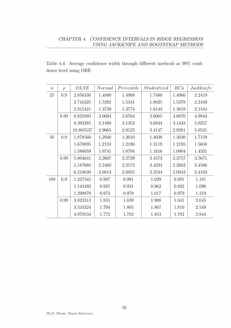
which is due to the consistency of the estimators. It is evident from Tables (4.3)

and (4.4) that the confidence intervals based on ORE have shorter widths in

comparison to the width of the interval based on OLSE.

It is interesting to note that the coverage probabilities and confidence width

through OLSE and through jackknife are very close to each other. Also, from

Tables (4.3) and (4.4), we find that with the increasing collinearity between

the dependent variables, the difference between the confidence width of inter-

val based on OLSE and intervals based on ORE is increasing. Also, with the

increasing value of sample size, the confidence width of all the intervals is de-

creasing.


86


According to Tables (4.1) and (4.2), all the bootstrap methods are generally

conservative in terms coverage probabilities, however jackknife method seems to

give coverage probabilities closer to the target. In terms of confidence width,

resampling methods have smaller confidence width than the OLSE; jackknife

method having larger confidence width than bootstrap methods. In noting that

bootstrap methods are conservative with smaller confidence width, they seem

to have an advantage over the jackknife method.

4.6 Concluding Remarks

In the present chapter, we illustrated the use of different confidence intervals

based on bootstrap and jackknife resampling methods. We obtained the cover-

age probabilities and confidence width based on ORE using different bootstrap

and jackknife method and compared it with that of OLSE which we computed

using t-intervals. The shorter confidence widths obtained through ORE shows

its superiority over OLSE in the case of multicollinearity. The next chapter

deals with jackknifing and bootstrapping another biased estimator given by Liu

[64] to overcome the drawback of ORE.


87


Table 4.1: Coverage Probabilities through different methods at 95% confidence

level

n ρ OLSE Normal Percentile Studentized BCa Jackknife

25 0.9 0.952 0.966 0.974 0.978 0.970 0.940

0.964 0.966 0.960 0.976 0.964 0.922

0.962 0.972 0.978 0.986 0.976 0.944

0.99 0.952 0.970 0.980 0.986 0.972 0.940

0.964 0.964 0.964 0.984 0.966 0.920

0.964 0.986 0.986 0.994 0.990 0.936

50 0.9 0.950 0.974 0.972 0.980 0.970 0.948

0.952 0.968 0.976 0.984 0.976 0.936

0.948 0.988 0.986 0.990 0.990 0.964

0.99 0.950 0.984 0.984 0.986 0.984 0.948

0.952 0.986 0.984 0.990 0.986 0.934

0.948 0.994 0.994 0.996 0.994 0.968

100 0.9 0.958 0.972 0.974 0.978 0.974 0.948

0.962 0.958 0.954 0.956 0.952 0.930

0.940 0.966 0.968 0.968 0.964 0.932

0.99 0.958 0.984 0.984 0.984 0.984 0.946

0.962 0.974 0.976 0.982 0.974 0.928

0.944 0.978 0.978 0.980 0.978 0.926


88


Table 4.2: Coverage Probabilities through different methods at 99% confidence

level


25 0.9 0.992 0.992 0.990 0.994 0.990 0.984

0.990 0.990 0.988 0.994 0.992 0.982

0.996 1.000 0.998 1.000 0.996 0.994

0.99 0.992 0.992 0.990 0.994 0.992 0.984

0.990 0.990 0.992 0.996 0.992 0.978

0.998 0.996 1.000 1.000 0.998 0.992

50 0.9 0.998 0.994 0.994 0.994 0.994 0.988

0.990 0.994 0.996 0.998 0.996 0.990

0.992 0.994 0.996 0.996 0.994 0.994

0.99 0.998 0.994 0.994 0.994 0.994 0.988

0.990 1.000 0.998 1.000 0.998 0.990

0.988 0.998 1.000 1.000 0.998 0.994

100 0.9 0.988 0.992 0.992 0.992 0.992 0.988

0.990 0.988 0.986 0.990 0.988 0.982

0.994 0.990 0.988 0.994 0.986 0.976

0.99 0.988 0.992 0.992 0.994 0.992 0.988

0.990 0.996 0.994 0.998 0.996 0.980

0.992 0.996 0.996 0.996 0.992 0.978


89


Table 4.3: Average confidence width through different methods at 95% confi-

dence level using OLSE and ORE


25 0.9 2.101518 1.1330 1.1346 1.2801 1.1361 1.6494

1.998510 1.1712 1.1732 1.3216 1.1738 1.6516

2.144994 1.0454 1.0475 1.1809 1.0483 1.5851

0.99 6.493567 2.3355 2.3407 2.6376 2.3437 3.6672

6.175280 2.3954 2.4000 2.7049 2.4008 3.6976

7.994216 2.2116 2.2146 2.5011 2.2178 3.7170

50 0.9 1.407747 0.9846 0.9864 1.0449 0.9868 1.2858

1.258123 0.9225 0.9241 0.9793 0.9245 1.1733

1.188554 0.8173 0.8185 0.8671 0.8191 1.0739

0.99 4.349856 1.7202 1.7245 1.8256 1.7251 2.6731

3.887527 1.7090 1.7124 1.8153 1.7128 2.5918

4.654095 1.5836 1.5854 1.6813 1.5869 2.5555

100 0.9 0.9346568 0.7506 0.7518 0.7732 0.7518 0.8923

0.8637652 0.7042 0.7053 0.7244 0.7057 0.8282

0.9818960 0.7410 0.7423 0.7639 0.7430 0.9207

0.99 2.888035 1.3929 1.3957 1.4355 1.3971 1.9978

2.668984 1.3652 1.3669 1.4057 1.3687 1.9255

3.754617 1.3487 1.3496 1.3918 1.3509 2.1479


90


Table 4.4: Average confidence width through different methods at 99% confi-

dence level using ORE


25 0.9 2.856330 1.4890 1.4908 1.7480 1.4960 2.2419

2.716325 1.5392 1.5341 1.8025 1.5378 2.2449

2.915421 1.3739 1.3774 1.6143 1.3819 2.1544

0.99 8.825893 3.0694 3.0764 3.6005 3.0870 4.9844

8.393285 3.1480 3.1353 3.6944 3.1443 5.0257

10.865537 2.9065 2.9123 3.4147 2.9281 5.0521

50 0.9 1.878560 1.2940 1.3010 1.4038 1.3030 1.7159

1.678895 1.2124 1.2190 1.3119 1.2195 1.5658

1.586059 1.0741 1.0794 1.1616 1.0804 1.4331

0.99 5.804641 2.2607 2.2739 2.4573 2.2757 3.5671

5.187688 2.2460 2.2573 2.4294 2.2602 3.4586

6.210630 2.0813 2.0925 2.2534 2.0943 3.4102

100 0.9 1.237342 0.987 0.991 1.029 0.991 1.181

1.143492 0.925 0.931 0.962 0.933 1.096

1.299879 0.974 0.979 1.017 0.979 1.219

0.99 3.823313 1.831 1.839 1.908 1.841 2.645

3.533324 1.794 1.803 1.867 1.810 2.549

4.970534 1.772 1.782 1.853 1.782 2.844


91

Chapter 4 Conﬁdence Intervals in Ridge Regression using Jackknife and Bootstrap...

Documents

Transcript of Chapter 4 Conﬁdence Intervals in Ridge Regression using Jackknife and Bootstrap...