Virginia Commonwealth University Virginia Commonwealth University

VCU Scholars Compass VCU Scholars Compass

Theses and Dissertations Graduate School

2009

Comparing Bootstrap and Jackknife Variance Estimation Comparing Bootstrap and Jackknife Variance Estimation

Methods for Area Under the ROC Curve Using One-Stage Cluster Methods for Area Under the ROC Curve Using One-Stage Cluster

Survey Data Survey Data

Allison Dunning Virginia Commonwealth University

Follow this and additional works at: https://scholarscompass.vcu.edu/etd

Part of the Biostatistics Commons

© The Author

Downloaded from Downloaded from https://scholarscompass.vcu.edu/etd/1849

This Thesis is brought to you for free and open access by the Graduate School at VCU Scholars Compass. It has been accepted for inclusion in Theses and Dissertations by an authorized administrator of VCU Scholars Compass. For more information, please contact libcompass@vcu.edu.

ii

COMPARING BOOTSTRAP AND JACKKNIFE VARIANCE ESTIMATION

METHODS FOR AREA UNDER THE ROC CURVE USING ONE-STAGE CLUSTER

SURVEY DATA

A Thesis submitted in partial fulfillment of the requirements for the degree of Master of

Science at Virginia Commonwealth University.

by

ALLISON MARIE DUNNING

B.S. Statistics, Virginia Tech, 2007

Director: CHRISTINE SCHUBERT, PH.D.

ASSISTANT PROFESSOR, DEPARTMENT OF BIOSTATISTICS

Virginia Commonwealth University

Richmond, VA

June 2009

ii

Acknowledgement

First I must acknowledge my family, without your support I would not be here

today. To my mother and father you have always been there for me, a constant source of

support. You believed in me even when I did not believe in myself. You never allowed

me to give up on myself and reminded me often that I could achieve anything I wanted.

To my sister Becky, your support the past two years has meant a lot. I thank you for

living with me these past two years and putting up will all my mood swings, it couldn’t

have been much fun. To my brother Andy, I have always looked up to you and I thank

you for your support over the years.

To Virginia Commonwealth University and especially the Department of

Biostatistics, I thank you for your financial support over the past two years. To my

professors, I thank you for the time you committed to furthering my education and the

support you have provided me over the past two years.

I must make special mention of my thesis advisor Dr. Schubert. Ever since my

entry to the department you have been looking out for me. I thank you for all your

guidance and support over the past two years and especially this last year working on my

iii

thesis. Without you this thesis would never have happened. You knew how to push me

in the right direction without being overbearing. I cannot express the gratitude I feel for

the countless hours of work you devoted to this project and to me. I really appreciate

everything you have done for me, and I will carry all our meetings over the past year with

me into the future.

I would also like to thank Dr. Sabo and Dr. McClish, your guidance over the past

year has been astonishing. I appreciate greatly the time you allowed me and the help you

provided it will not be forgotten.

I would like to acknowledge the 32 students and faculty of Virginia Tech who lost

their lives April 16, 2007. That event has forever changed my life. Two years ago as I

entered my graduate work following this event I could not imagine how I was to achieve

anything with the anguish left by my fallen peers and mentors. But as Nikki Giovonni

stated in her poem “We will Prevail”, I have done just that. Through the support of my

friends and family and Hokie spirit I have prevailed and accomplished something that

two years ago seemed impossible. You will never be forgotten.

iv

Table of Contents

ACKNOWLEDGEMENT............................................................................................... II

LIST OF TABLES ..........................................................................................................VI

LIST OF FIGURES ...................................................................................................... VII

ABSTRACT..................................................................................................................VIII

1. INTRODUCTION......................................................................................................... 1

1.1 Motivation and Purpose ........................................................................................ 1

1.2 Previous Studies ..................................................................................................... 3

1.3 Outline of Thesis .................................................................................................... 5

2. METHODS .................................................................................................................... 7

2.1 Survey Design.............................................................................................................. 7 2.1.1 One Stage Cluster Sampling .................................................................................. 9 2.1.2 National Health and Nutrition Examination Survey (NHANES) ........................ 11

2.2 Receiver Operator Characteristic (ROC) Curves ................................................. 15 2.2.1 Logistic Regression .............................................................................................. 15 2.2.2 Receiver Operator Characteristic (ROC) Curves ................................................. 18 2.2.3 Area under the ROC Curve (AUC) ...................................................................... 21

2.3 Variance Estimation Methods ................................................................................. 25 2.3.1 Bootstrap .............................................................................................................. 27

v

2.3.2 Jackknife............................................................................................................... 30

3 RESULTS ..................................................................................................................... 33

3.1 Simulated Data .......................................................................................................... 33 3.1.1 Simulated Data Introduction ................................................................................ 35 3.1.2 Simulated Data: Methods ..................................................................................... 37 3.1.3 Simulated Data Results ........................................................................................ 41 3.1.4 Simulated Data Conclusions ................................................................................ 50

3.2 NHANES Data........................................................................................................... 51 3.2.1 NHANES Data Introduction ................................................................................ 51 3.2.2 NHANES Methods............................................................................................... 55 3.2.3 NHANES Results................................................................................................. 58 3.2.4 NHANES Conclusions......................................................................................... 62

4 DISCUSSION AND FUTURE WORK...................................................................... 63

BIBLIOGRAPHY........................................................................................................... 66

APPENDIX...................................................................................................................... 68

VITA............................................................................................................................... 108

vi

List of Tables Table 1……………………………………………………………………………………............16 Table 2 NHANES Results ............................................................................................................. 58 

vii

List of Figures

page

Figure 1: Bootstrap and Jackknife AUC Estimates vs. True Area ......................................1

Figure 2: Bootstrap and Jackknife AUC Estimates vs. Prevalence .....................................1

Figure 3: Jackknife vs. Bootstrap Variance Estimates for 2 Clusters..................................1

Figure 4: Jacknife vs. Bootstrap Variance Estimates...........................................................1

Figure 5: Jackknife vs. Bootstrap Variance Estimates for 5 Clusters..................................1

Figure 6: Jackknife vs. Bootstrap Variance Estimates for 7 Clusters..................................1

Figure 7: Log Bootstrap Variance Estimates vs. True Area, Prevalence, & Clusters .........1

Figure 8: Log Jackknife Variance Estimates vs. True Area, Prevalence, & Clusters..........1

Figure 9: NHANES AUC Estimates vs. Hormones...........................................................60

viii

Abstract  

 

COMPARING BOOTSTRAP AND JACKKNIFE VARIANCE ESTIMATION METHODS FOR AREA UNDER THE ROC CURVE USING ONE-STAGE CLUSTER SURVEY DATA

By Allison M. Dunning M.S.

A thesis submitted in partial fulfillment of the requirements for the degree of Master of Science at Virginia Commonwealth University.

Virginia Commonwealth University, 2009

Major Director: Christine Schubert, Assistant Professor Department of Biostatistics

The purpose of this research is to examine the bootstrap and jackknife as methods for

estimating the variance of the AUC from a study using a complex sampling design and to

determine which characteristics of the sampling design effects this estimation.

Data from a one-stage cluster sampling design of 10 clusters was examined. Factors

included three true AUCs (.60, .75, and .90), three prevalence levels (50/50, 70/30,

90/10) (non-disease/disease), and finally three number of clusters sampled (2, 5, or 7). A

simulated sample was constructed for each of the 27 combinations of AUC, prevalence

and number of clusters.

ix

Estimates of the AUC obtained from both the bootstrap and jackknife methods

provide unbiased estimates for the AUC. In general it was found that bootstrap variance

estimation methods provided smaller variance estimates. For both the bootstrap and

jackknife variance estimates, the rarer the disease in the population the higher the

variance estimate. As the true area increased the variance estimate decreased for both the

bootstrap and jackknife methods. For both the bootstrap and jackknife variance

estimates, as number of clusters sampled increased the variance decreased, however the

trend for the jackknife may be effected by outliers.

The National Health and Nutrition Examination Survey (NHANES) conducted by the

CDC is a complex survey which implements the use of the one-stage cluster sampling

design. A subset of the 2001-2002 NHANES data was created looking only at adult

women. A separate logistic regression analysis was conducted to determine if exposure

to certain furans in the environment have an effect on abnormal levels of four hormones

(FSH, LH, TSH, and T4) in women.

Bootstrap and jackknife variance estimation techniques were applied to estimate the

AUC and variances for the four logistic regressions. The AUC estimates provided by

both the bootstrap and jackknife methods were similar, with the exception of LH. Unlike

in the simulated study, the jackknife variance estimation method provided consistently

x

smaller variance estimates than bootstrap. AUC estimates for all four hormones

suggested that exposure to furans effects abnormal levels of hormones more than

expected by chance.

The bootstrap variance estimation technique provided better variance estimates for

AUC when sampling many clusters. When only sampling a few clusters or as in the

NHANES study where the entire population was treated as a single cluster, the jackknife

variance estimation method provides smaller variance estimates for the AUC.

 

1

1. Introduction 1.1 Motivation and Purpose

Survey samples are becoming an increasingly popular method to obtain information.

With the introduction of the internet and in particular email, there is virtually no limit to

the number of people who can now be reached. Everyday millions of inboxes are filled

with requests to fill out an online survey. In conjunction with this growing technology

and improving ability to reach people, statistically valid surveys are also being developed

and the ability to administer these surveys is monumentally easier than in years past; thus

the popularity of these surveys is also increasing.

Such surveys often implement the use of complex sampling designs. For

example, the Centers for Disease Control (CDC) conduct the National Health and

Nutrition Examination Survey (NHANES), which uses a one-stage cluster sampling

approach. Obtaining estimates, and in particular their variances, requires special

considerations. For example, if one wishes to perform a logistic regression analysis on

data collected from NHANES, one estimate that can be used to summarize this analysis is

the area under the receiver operator characteristic (ROC) curve. Such an estimate must

incorporate appropriate adjustments specific to the sampling design. Special techniques

exist to estimate these values as well as their variances. Two popular techniques are the

bootstrap and jackknife variance estimation methods. These two techniques are part of a

larger group known as replication methods.

2 

 

The purpose of this research is to use these replication methods to create estimates

for the variances of area under the ROC curve (AUC) obtained from data collected using

one-stage cluster sampling designs. In particular, this research will focus on comparing

the bootstrap and jackknife variance estimation methods. It will be of interest to

determine if certain factors related to the sample and the sampling design affect these

variance estimates. In addition to the calculation of the AUC for data obtained from

NHANES, data will be simulated so as to test the effect of three factors related to the

sample and sampling design on the variance estimates from both methods. The three

factors to be tested are true AUC, prevalence of disease, and number of clusters sampled.

A comparison of the two methods will be performed using simulated data. Finally these

methods will be used to analyze data obtained from NHANES.

3 

 

1.2 Previous Studies

A discussion will now follow of previous work comparing variance estimation

techniques in complex surveys. It is important to note that while studies have been

conducted to compare variance techniques for complex surveys, these studies have yet to

be extended to AUC.

A study published in 1996 by Rust and Rao examined data obtained from

NHANES. Replication based variance estimation methods such as the bootstrap and

jackknife have been suggested to “confront the fact that the sample design, …, impacts

the level of error associated with estimates obtained from the data” (Rao). Studies, such

as those done by Kovar et al, have shown that both the bootstrap and jackknife methods

provide similar results when looking at linear estimators (Rao). Kovar et al also showed

that the jackknife method had lower mean square error as an estimator of the sampling

variance.

Several publications have looked at comparing the jackknife technique to another

replication method known as balanced repeated replication (BRR). It should be noted

that in Rust 1985, the BRR method has been shown to be similar to the bootstrap method

in terms of variance estimates behavior (Rust). A paper published in 1985, this time by

Rust alone, compared variance estimation for complex estimators in sample surveys. In

4 

 

this paper, Rust compared the jackknife method with the BRR method. Rust found that

that the BRR method performed better than the jackknife in variance estimation of

population estimates from sample surveys. The work of Kish and Frankel looked at

comparing these methods for estimation of ratios. This study found that BRR provided

the best coverage in terms of confidence intervals calculated around the estimates for the

ratios. Cambell and Meyer also compared BRR and jackknifing for variance estimation.

Their results agreed with Kish and Frankels findings that BRR provided the best

confidence intervals. It also found that BRR gave better performance across a variety of

population conditions.

These studies would suggest that perhaps the jackknife procedure will not

perform as well as other replication techniques. However, these studies have focused on

specific population estimates, such as ratios, and have yet to look at how these replication

methods will behave when used to estimate AUC and its variance. This research is the

first step in examining how these previous results compare to those proposed in this

research for AUC.

5 

 

1.3 Outline of Thesis

The purpose of this thesis is to compare the bootstrap and jackknife variance

estimation techniques in estimating the variance of AUC for data collected using one-

stage cluster sampling designs. This will be accomplished by first applying both

techniques to simulated data. This simulated data will be structured to look at the effect

of true population AUC, prevalence of disease and number of clusters sampled on both

estimation techniques. The techniques will then be compared using the results from the

simulated data study. Finally, both techniques will be applied to data collected from

NHANES in order to both compare the provided variance estimates by both techniques

and to determine whether or not exposure of the US population to harmful chemicals

effect hormone levels in women.

Before these variance estimation techniques can be applied, the research methodology

will be discussed. First, a discussion of survey design will be given. This will include an

overview of one-stage cluster sampling designs. Then, a discussion of NHANES will

outline how this survey is conducted and how its data is structured for analysis.

Background of the ROC curve will be provided, including an introduction to logistic

regression analysis and how the ROC curve is calculated. A discussion on summary

measurements for the ROC curve is given, focusing in particular on the area under the

ROC curve. Finally, the methodology concludes with a discussion of variance estimation

methods, including detailed descriptions of the bootstrap and jackknife variance

estimation techniques.

6 

 

Following the methodology, the data will be introduced. A description of the

simulated data will be given. This will include full details of how the simulated data is

structured and how it was created. Further, the NHANES data will be described

including what variables were collected, and how they were collected. A logistic

regression analysis will be introduced to determine if exposure to ten furans has an effect

on reproductive and thyroid hormone levels in women. Once the data has been

introduced, the results will be presented. A discussion of the methods used will include a

description of how the bootstrap and jackknife techniques were applied to both the

simulated data and the NHANES data. Finally, the results from the simulated data and

NHANES are presented. The results for the NHANES data will not only include the

comparison of the two variance estimation techniques but also the results of the research

question. Conclusions and discussion of implications of the research is then presented.

This will include suggestions for future work.

 

7

2. Methods

2.1 Survey Design

Survey analysis is typically conducted as if all sample observations were

independently selected with equal probabilities; however, in practice the sample selection

is more complex. Often with survey data some subjects may be selected with higher

probability than others. Also, some subjects are included in the sample simply because of

their membership in a certain group, as in a cluster sample. So the question arises, “What

special methods and computer programs are available for the more appropriate analysis

of complex survey data?” Implementing typical survey analysis under the assumption of

simple random sampling with replacement on surveys that employs stratification and

clustering of observations along with unequal selection probabilities can lead to bias and

misleading results (Lee). This is due in part to the complex survey design, which is

defined as any survey that has restrictions on the sampling other than the simple random

sample with replacement assumption. These complex designs require special

consideration when analyzed. Some examples of complex survey designs are those

surveys that implement stratification or cluster sampling, or a combination of both.

Stratification employs the use of scientifically identified groups known as strata, to split

the population into different groups for analysis. Cluster sampling employs the use of

clusters to split the population into convenient and cost effective groups, not necessarily

considering the differences between the groups. Many large scale population studies use

8 

 

such cluster designs to efficiently organize the study. The focus of this research will be

on cluster sampling techniques.

9 

 

2.1.1 One Stage Cluster Sampling

One type of complex survey sampling design is cluster sampling. In cluster

sampling, one chooses observations by groups of elements (called clusters) rather than by

individual elements. An advantage is that cluster sampling can reduce survey costs when

acquiring information on groups or clusters is easier and less expensive than obtaining

information for individuals. All survey methods still require the use of a sampling frame

which lists all possible elements available for the study. Unfortunately it is sometimes

difficult to find a good frame for listing population elements. However, a frame listing

clusters may be readily available. For example, if a study is interested in interviewing

individuals in a certain city living in apartments, a listing of all residents in the city may

not be available. However one could easily obtain a listing of apartment buildings in the

city. The apartment buildings could then be used as clusters.

Often in complex surveys the sample sizes for each cluster or group are not equal.

In such cases, elements in the smaller clusters are more likely to be chosen for the sample

over the larger clusters. Also in certain complex designs, the clusters may be stratified

according to certain survey objectives. This use of disproportionate stratification and

unequal sized clusters complicates the estimation process (Lee).

To obtain a cluster sample, the first task is to specify the clusters to be used.

Typically measurements within a cluster are correlated. Therefore the amount of

information contained from one element in a cluster about a population parameter may

10 

 

not be substantial. However, it is not uncommon to come upon the situation where

elements within a cluster are very different from one another. One example may be

dorms on a college campus, for which one would expect residents to differ in some way.

In the case where the elements in a cluster are similar, more information may be gathered

by sampling a larger number of clusters of smaller size. When considering a cluster

sample it is important to note the differences in the construction of a stratum versus a

cluster. As previously noted, strata are typically very different from one another with

respect to characteristics being measured; however, elements within a stratum are to be as

homogeneous as possible. On the other hand, clusters should be as heterogeneous as

possible within, and one cluster should be very much like another to take full advantage

of the cost efficiency of cluster sampling. This is so each cluster is representative of the

true population. It also reduces variability. Once a sampling frame of clusters is

obtained, a simple random sample of those clusters is chosen. Then all elements in every

selected cluster are sampled for inclusion in a study or survey. Issues surrounding the

homogeneity within and between clusters as well as sample sizes within a cluster must be

considered in variance estimates of population parameters.

The next section will describe one survey that implicates the use of cluster

sampling, the National Health and Nutrition Examination Survey (NHANES).

11 

 

2.1.2 National Health and Nutrition Examination Survey (NHANES)

The National Health and Nutrition Examination Survey (NHANES) is a program

of studies designed to assess the health and nutritional status of adults and children in the

United States, conducted by Centers for Disease Control (CDC). The NHANES program

began in the early 1960s and has been conducted several times as a series of surveys

focusing on different population groups or health topics until the 1990’s. Since 1999, the

survey has been conducted continuously with data being combined in two year intervals.

The survey is unique in that it combines interviews and physical examinations. The

CDC makes this collected data available, both from interviews and physical

examinations, for use by the public and other health organizations on their website.

NHANES is conducted by first splitting the country into counties, which serve as

primary sampling units and using these counties as a sampling frame. Of the many

counties across the country, 15 are selected to be visited each year. Clusters of

households are selected, each person in a selected household is screened for demographic

characteristics, and one or more persons per household are selected for the sample. This

research uses, NHANES 2001-2002, for which there were 13,156 persons selected for the

sample; 11,039 of those were interviewed (83.9%) and 10,477 (79.6%) were examined in

the NHANES mobile examination center (MEC). The NHANES interview includes

demographic, socioeconomic, dietary, and health-related questions. In addition, the

examination component consists of medical, dental, and physiological measurements, as

well as laboratory tests, which are administered by highly trained medical personnel.

12 

 

Health interviews are conducted in respondents’ homes, and health measurements are

performed in specially designed and equipped mobile centers, which travel to the

designated locations throughout the country. The mobile center staff automatically

transmit data into databases where it is available to CDC staff. Survey information is

available to CDC staff within 24 hours of collection. This quick data collection and

submission enhances the capability of collecting quality data and increases the speed with

which results are released to the public.

The sample for the survey is selected to represent the non-institutionalized U.S.

population of all ages, meaning that both children and adults are selected to be questioned

and examined. The tests and procedures performed in the examination depend on the age

of the participant; in general, older individuals receive more extensive examinations. All

participants visit the physician, give dietary interviews and have body measurements

taken, and all but the very young have blood taken and a dental screening. Participants of

NHANES receive compensation and a report of medical findings, and all information

collected in the survey is kept strictly confidential.

The National Institutes of Health (NIH), the Food and Drug Administration

(FDA) and CDC are among the agencies that rely upon NHANES to provide data

essential for the implementation and evaluation of program activities (Services).

Findings from the NHANES survey are used to determine the prevalence of major

diseases and risk factors for diseases, and chronic conditions in the population. Risk

factors, those aspects of a person’s lifestyle, constitution, heredity, or environment that

13 

 

may increase the chances of developing a certain disease or condition, are examined.

Past surveys have provided data to create growth charts used nationally by pediatricians

to evaluate children’s growth. Blood lead data were instrumental in developing policy to

eliminate lead from gasoline, food and soft drink cans, resulting in a decline in elevated

blood levels by more than 70% since the 1970s (Services). Data have continued to

indicate that undiagnosed diabetes is a significant problem in the United States. Facts

about the distribution of health problems and risk factors in the population give

researchers important clues to the causes of disease. From the NHANES survey, the

CDC can identify the health care needs of the population, from which government

agencies and private sector organizations can establish policies and plan research,

education, and health promotion programs to help improve present health status and

prevent future health problems.

One problem with analyzing the NHANES data is the complex survey structure.

NHANES is described by the CDC as a complex sample survey. Data collected comes

from interviews, examinations, and laboratory tests based on blood and urine samples.

Dust or tap water samples may also be collected in the home. The source of a data item

is important for both assessment of quality of information and for determining the

appropriate sampling weights. Interview data, while administered by a trained NHANES

member, are based on self reporting and are therefore subject to non-sampling errors,

such as recall problems, and misunderstanding of the question, among other factors.

Examination data and laboratory data are subject to measurement variation and possible

14 

 

examiner effects. To help reduce these errors, prior to and during data collection,

NHANES field staff participates in comprehensive training and annual refresher training

for interviewers and MEC staff. The primary sampling units (PSUs) for the NHANES

survey are generally single counties, although small counties are sometimes combined to

meet a minimum population size. Because NHANES is a complex probability sample,

analytic approaches based on data from simple random samples are usually not

appropriate. As with any complex probability sample, the sample design information

should be explicitly used when producing statistical estimates or undertaking statistical

analysis of the NHANES data. Ignoring the complex design can lead to biased estimates

and overstated significance levels. Sample weights and the stratification and clustering

of the design must be incorporated into an analysis to get proper estimates and standard

errors of estimates.

15 

 

2.2 Receiver Operator Characteristic (ROC) Curves

2.2.1 Logistic Regression

Often when looking at survey data the responses are categorical, whether binary

(having two outcomes), nominal, (having several unordered outcomes) or ordinal (having

several ordered outcomes). To examine the association among variables methods using

categorical response variables are necessary. Logistic regression is a commonly used

analysis method when conducting surveys, as it is used to examine the association of a

categorical outcome or response with a number of independent variables (Lee).

Specifically, logistic regression is a way of converting the proportions or rates of

categorical data into numbers that have real interpretations. For example, logistic

regression is commonly used when the outcome or response is the presence or absence of

a condition, often a disease. In these cases, the explanatory variable is often a test or

procedure used to detect this condition. Logistic regression allows us to convert these

agreement proportions into probabilities of having the disease. In addition, these

probabilities can be converted into sensitivity and specificity which can be used to

determine the accuracy of a procedure or test in successfully predicting the absence or

presence of a condition. Sensitivity is the probability that the test correctly identifies a

diseased patient with the disease and specificity is the probability that the test correctly

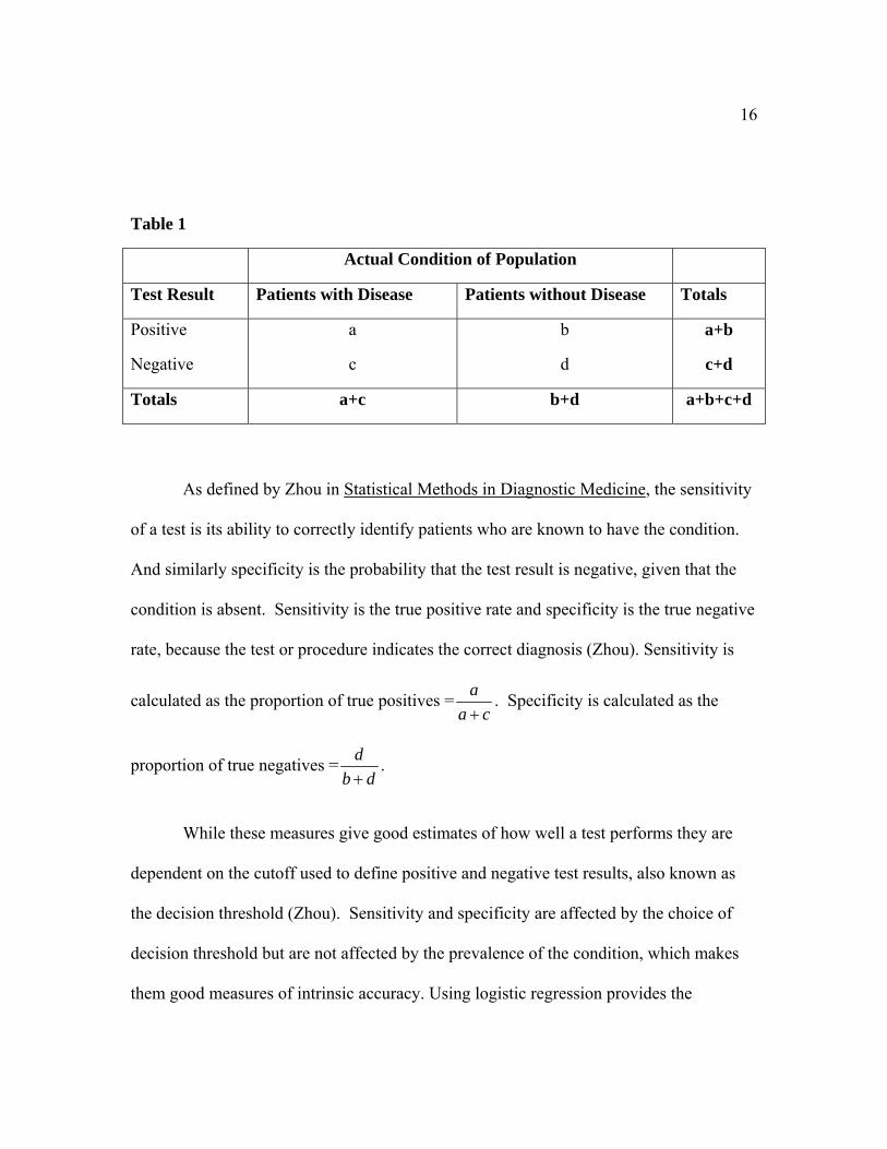
identifies the non-disease patients without the disease. Table 1 below helps demonstrate

the idea of sensitivity and specificity and how they are calculated.

16 

 

Table 1

Actual Condition of Population

Test Result Patients with Disease Patients without Disease Totals

Positive

Negative

a

c

b

d

a+b

c+d

Totals a+c b+d a+b+c+d

As defined by Zhou in Statistical Methods in Diagnostic Medicine, the sensitivity

of a test is its ability to correctly identify patients who are known to have the condition.

And similarly specificity is the probability that the test result is negative, given that the

condition is absent. Sensitivity is the true positive rate and specificity is the true negative

rate, because the test or procedure indicates the correct diagnosis (Zhou). Sensitivity is

calculated as the proportion of true positives = aa c+

. Specificity is calculated as the

proportion of true negatives = db d+

.

While these measures give good estimates of how well a test performs they are

dependent on the cutoff used to define positive and negative test results, also known as

the decision threshold (Zhou). Sensitivity and specificity are affected by the choice of

decision threshold but are not affected by the prevalence of the condition, which makes

them good measures of intrinsic accuracy. Using logistic regression provides the

17 

 

sensitivity and specificity of a procedure or test at all decision thresholds giving an idea

of how well a test performs over the entire range of decision thresholds.

18 

 

2.2.2 Receiver Operator Characteristic (ROC) Curves

From logistic regression a graph in which the Y-axis represents sensitivity and the

X-axis represents 1 minus specificity can be obtained for every possible threshold. This

plot is the Receiver Operator Characteristic or ROC curve. An ROC curve is a way of

describing the intrinsic accuracy of a test apart from the decision thresholds. Since the

1970s, the ROC curve has been the most valuable tool for describing and comparing

diagnostic tests and procedures (Zhou). It is interesting to note that the name “receiver

operator characteristic” curve comes from the notion that given the curve, we – the

receivers of the information – can use (or operate at) any point on the curve by using the

appropriate decision threshold (Zhou). As stated above, the sensitivity and specificity of

a procedure or test is independent of disease prevalence, and since the ROC curve is a

plot of these measurements, it too is independent of disease prevalence. Also, the ROC

curve has the advantage of being invariant to monotonic transformations, as it does not

depend on the scale of the test results (Zhou).

ROC curves can be constructed from either objective or subjective measurements.

However, regardless of the type of decision threshold the curve has the same

interpretation; it illustrates the trade-off between the sensitivity and false positive rate as

the decision threshold changes. For measurements that are made objectively, the decision

variable is explicit, so one can choose from an infinite number of decision thresholds

along the continuum of test results. Also for diagnostic tests interpreted subjectively, the

19 

 

decision thresholds are implicit or latent, for they exist only in the mind of the observer

(Zhou).

A procedure or test that cannot discriminate between presence and absence of a

condition will provide an ROC curve which is a forty-five degree line passing through

the origin with slope of one (Giulia Bisoffi). The best tests have high sensitivity and low

1- specificity. Correspondingly, effective tests or procedures will provide a convex curve

above this line. Specifically the ROC curve gives the precise magnitude at which the

false positive rate increases as the sensitivity increases (Zhou). Assuming the statistical

model used for the disease and non-disease populations has a binormal distribution, as it

is the most commonly used model for fitting ROC curves in diagnostic medicine, the

curve is then completely specified by two parameters, “a” and “b”. A binormal

distribution assumed that both the non-disease and disease populations are normally

distributed with different means and standard deviations

( ) ( )2 2, ,,disease N non disease ND NDD NDμ σ μ σ⎛ ⎞−⎜ ⎟⎝ ⎠

: : Where ‘a’ is the standardized

difference in means of the distributions of the test results for patients with and without

the condition; and ‘b’ is the ratio of the standard deviations of the test results for patients

without versus with the condition (Zhou).

Through the use of logistic regression, a statistical model can be fit to the test

results of a sample of subjects producing a fitted ROC curve (or smooth curve) (Zhou).

This is in contrast to the empirical ROC curve which only uses the observed data.

20 

 

Assuming they are on two similar scales one can compare two ROC curves. For

example, it may be of interest to compare two testing procedures on their accuracy of

correctly diagnosing the same disease. It may be of interest to compare the two ROC

curves. In situations like this, it is helpful to have a single number to compare the curves.

In the following section we will talk about one such summary for ROC curves known as

the area under the ROC curve (AUC).

21 

 

2.2.3 Area under the ROC Curve (AUC)

The area under the ROC curve (AUC) is a single number summary of an ROC

curve that one can use to compare the effectiveness of two separate diagnostic tests or

procedures. It is easier to compare a single number than to compare both the sensitivities

and specificities of the two tests (Zhou). When presented with two tests/procedures

used in detecting a certain condition it is not always feasible to simply directly compare

two ROC curves. It may be that the two curves are very similar making it hard to detect

which is better. Therefore rather than compare two ROC curves visually, the AUC for

the two ROC curves are compared. As such, the AUC is “the most common quantitative

index describing an ROC curve” (Hanley).

There are two methods for computing estimates of the AUC. These depend on the

assumptions regarding the underlying distributions of the two populations for those with

and without the condition. If binormality of the two populations is assumed then a

generally unbiased estimate for AUC can be obtained. In this case the area under the

smooth or fitted ROC curve is calculated as:

21

aAb

⎛ ⎞⎜ ⎟= Φ⎜ ⎟+⎝ ⎠

1.1

Where ( )Φ is the cumulative normal distribution, ( )D NDaD

μ μσ−

= and

NDbD

σσ

= (Zhou).

22 

 

In this case μND and σND represent the mean and standard deviation of the population of

subjects without the condition and μD and σD represent the mean and standard deviation

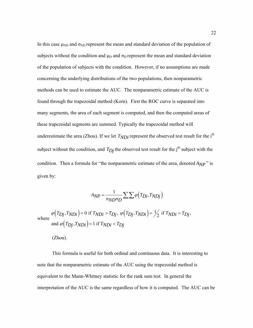
of the population of subjects with the condition. However, if no assumptions are made

concerning the underlying distributions of the two populations, then nonparametric

methods can be used to estimate the AUC. The nonparametric estimate of the AUC is

found through the trapezoidal method (Korn). First the ROC curve is separated into

many segments, the area of each segment is computed, and then the computed areas of

these trapezoidal segments are summed. Typically the trapezoidal method will

underestimate the area (Zhou). If we let TNDi represent the observed test result for the ith

subject without the condition, and TDj the observed test result for the jth subject with the

condition. Then a formula for “the nonparametric estimate of the area, denoted ANP ” is

given by:

( )1 ,A T TNP Di NDjn nND Dϕ= ∑∑

where ( ) ( )

( )1, 0 if , , if , 2

and , 1 if

T T T T T T T TDj NDi NDi Dj Dj NDi NDi Dj

T T T TDj NDi NDi Dj

ϕ ϕ

ϕ

= > = =

= <

(Zhou).

This formula is useful for both ordinal and continuous data. It is interesting to

note that the nonparametric estimate of the AUC using the trapezoidal method is

equivalent to the Mann-Whitney statistic for the rank sum test. In general the

interpretation of the AUC is the same regardless of how it is computed. The AUC can be

23 

 

interpreted in several ways. The most popular interpretation is that the AUC is the

probability that a randomly chosen subject with the condition of interest has a

test/procedure result indicating greater suspicion than that of a randomly chosen subject

without the condition of interest. Another interpretation of the AUC is that it is the

average value of sensitivity (specificity) for all possible values of specificity (sensitivity)

(Zhou). As stated previously, the ROC curve is invariant to the prevalence of the

condition and therefore the AUC is also invariant to the prevalence of the condition.

Therefore, the ROC curve area is simply a description of a test’s inherent ability to

discriminate between subjects with versus without the condition (Zhou).

The AUC takes on values between 0 and 1, since the ROC is a plot of

probabilities bounded by 0 and 1. Although the true range is between 0 and 1, we expect

by chance a test to correctly detect a condition about 50% of the time. Thus the practical

lower bound of AUC is 0.5. An area of 1.0 means that a test or procedure is performing

perfectly, so that the test or procedure correctly diagnoses each patient as having or not

having the condition. A diagnostic test or procedure when the ROC curve falls above the

chance line (has an AUC greater than 0.5) will have at least some ability to discriminate

between patients with and without the condition (Zhou).

Finally it is commonly of interest to compare two testing procedures and their

ability to correctly diagnose patients to the same condition. If the population is known,

then one can test if the two ROC curves are exactly the same with the hypothesis:

: , vs. : ,0 1H a a b b H a a b bND D ND D ND D ND D= = ≠ ≠

24 

 

Another way to compare these procedures is to compare their respective AUCs.

In order to determine if the two AUCs are significantly different the variances of both

ROC area estimates must be taken into account. Some methods for estimating these

variances are discussed in the next section.

25 

 

2.3 Variance Estimation Methods

Estimates of variances are necessary to evaluate the significance of the AUC

statistic. For complex estimators such as the AUC statistic used in sample surveys,

special difficulties arise in the estimation of the variance. Such difficulties could be that

the variance of the estimate may not be a linear or even known function of the population

parameters (Levy). Unique to survey designs, a researcher who wishes to analyze data

and compute appropriate variance estimates from a complex sample survey must

overcome three major issues in the data: (1) the presence of survey weights in the data,

(2) non-response and (3) the sample design, with the weighting adjustments for non-

response compensation and post-stratification. These issues will impact the level of error

associated with any estimates obtained from the data (Rao). There are a variety of

approaches that can be taken to deal with the impact of the design and estimation features

of the survey on the inference of the population parameter.

The assumptions associated with the underlying population of interest determine

which methods can be used to estimate the variance of an AUC estimate. If one assumes

binormality of the underlying distributions, variance can be computed using typical

variance estimation methods using linear estimates. When inferences about the

parameters of a finite population are based on sample survey data without model

assumptions, other methods must be used to derive estimates of the variances of the

parameter estimates (Rust). One technique is replication, in which the variance of the

26 

 

parameter estimator is obtained from the variability of estimates derived from different,

comparable parts of the original sample (Rust). These methods, once thought to be too

tedious and difficult to perform, have recently grown in popularity with the

implementation of computer algorithms.

“Replication is a general class of methods in which an estimate of the variance of

an estimated population parameter is obtained by expressing the estimated population

parameter as a sum or mean of several statistics, each of which is based on a subset of the

sample observations. One can obtain an estimate for the variance of the estimated

population parameter by calculating the variance of these “part sample” statistics”

(Levy). Hansen et al in a 1950s textbook first referred to these replication techniques as

random group methods. In current literature replication methods are sometimes called

resampling methods.

Replication methods estimate the sampling variance of a statistic by computing

the statistic for subsets of the sample and examining its variability over the subsets

(Levy). All replication techniques use computational intensity to overcome difficulties

and inconveniences in utilizing an analytic solution to the problem at hand (Rao).

Two popular replication methods include the bootstrap and the jackknife. In the

following two sections the bootstrap and jackknife variance estimation procedures are

outlined. Later, a discussion and comparison of the two methods is conducted to

determine how each performs in estimating the variance of the AUC statistic from a one-

stage cluster survey.

27 

 

 

2.3.1 Bootstrap

The bootstrap is one replication method that can be used for variance estimation

in sample surveys. The name bootstrap derives from the phrase “to pull oneself up by

one’s bootstrap” (Efron). The bootstrap was introduced in 1979 as a computer based

method for estimating variance. Because of modern technological breakthroughs, the

bootstrap has been developed more recently because the modern computer power it

requires to simplify intricate calculations (Efron).

The general idea of the bootstrap is to create artificial datasets with the same

structure and sample size as the original data. To create these artificial datasets simple

random samples are taken from the original with replacement, so that the same PSU may

be chosen multiple times and included in the same artificial or pseudo sample. Once the

artificial datasets are chosen, an estimate, *bθ of the parameter of interest,θ is calculated

from each pseudo sample. Then an estimate of the variance of the parameter of interest is

calculated as follows for the bootstrap:

( )2

1 * *( )1 1

BVarBS bB b

θ θ θ= −− =∑

where B is the number of replicate samples and 1* *

1

BbB b

θ θ==∑ .

28 

 

The issue of how many replicates is required to provide an acceptable variance

estimate arises. This problem is not trivial since the precision of the variance estimator

continues to increase as the number of replicates increases, but the resources needed to

carry out the bootstrap method obviously increases as well (Rao). It has been suggested

that the number of replicate samples needs to be large. Efron states that a large B would

be 200 replicates, however if confidence intervals will be calculated then it has been

suggested that B needs to be 1000 (Efron). While most literature when describing the

appropriate number of replicates reference Efron who says for just variance estimation B

= 200 is efficient, several studies have been done showing that perhaps this standard is

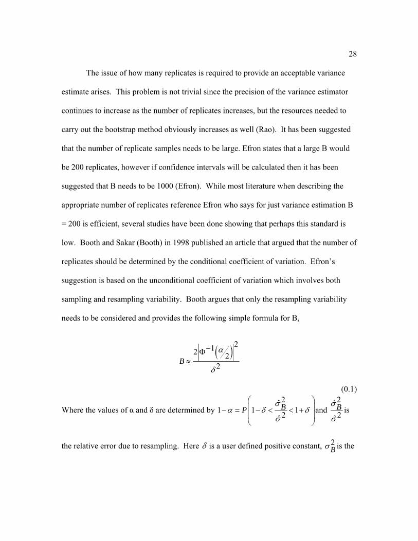
low. Booth and Sakar (Booth) in 1998 published an article that argued that the number of

replicates should be determined by the conditional coefficient of variation. Efron’s

suggestion is based on the unconditional coefficient of variation which involves both

sampling and resampling variability. Booth argues that only the resampling variability

needs to be considered and provides the following simple formula for B,

( ) 212 22Bα

δ

−Φ≈

(0.1)

Where the values of α and δ are determined by 2ˆ

1 1 12ˆBP

σα δ δ

σ

⎛ ⎞⎜ ⎟− = − < < +⎜ ⎟⎝ ⎠

and 2ˆ2ˆBσ

σis

the relative error due to resampling. Here δ is a user defined positive constant, 2Bσ is the

29 

 

bootstrap approximation of the variance and 2σ is the true variance. This formula

requires approximately 800 replicates to achieve a relative error less than 10% with

probability .95 (Booth). However when considering confidence intervals, Booths’ article

calculates a required B similar to Efron’s B = 1000. This research will use B=800

bootstrap replicates.

30 

 

2.3.2 Jackknife

The second replication-based variance estimator discussed here is the jackknife.

Jackknifing is another method for estimating the variance of estimates obtained from

complex sample surveys. As a replication based technique it is calculated using the

estimates of the parameter of interest for several part samples and then the variance is

found using these estimates. Unlike the bootstrap, the jackknife has a longer history

originating in 1956 with Quenoille. Tukey in 1958 extended the definition to say that the

technique could be adapted to produce variance estimates for many estimators (Rust). In

particular, the jackknife method can be used to estimate the variance of parameters from

complex sample survey data. A result of this long history is that there now exist several

variations to the jackknife procedure (Levy). The use of the jackknife procedure requires

the data to be split into groups. A single jackknife replicate is created by removing from

the sample all units associated with a given PSU from one group and inflating the

weights of all other units from the same group (Rao).

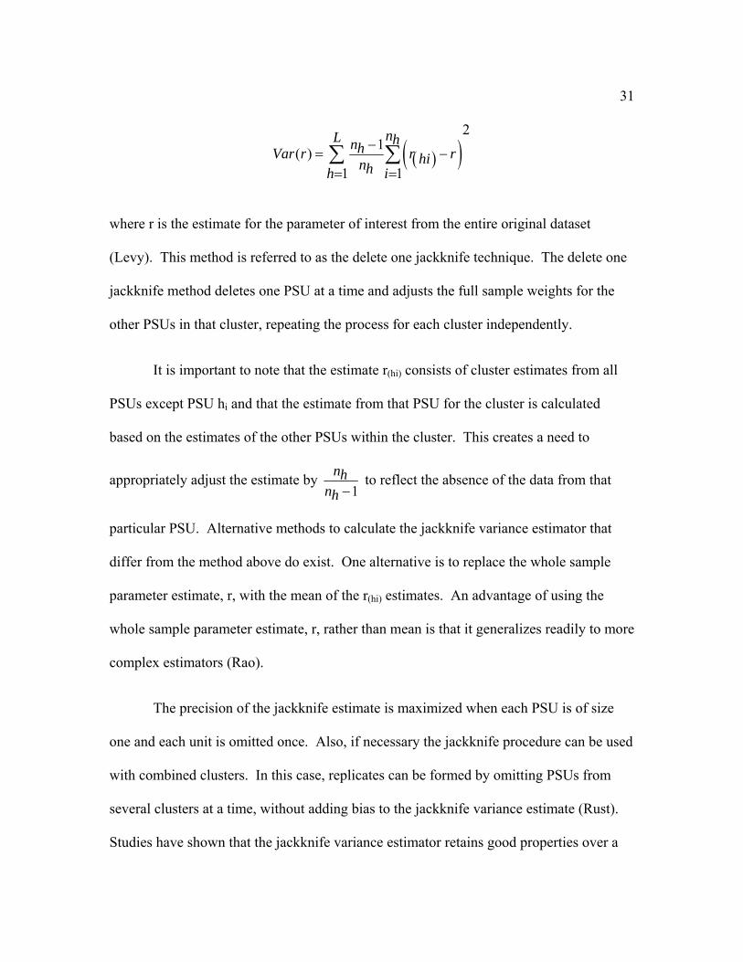
To find the jackknife variance estimate, suppose the data is composed of L

clusters, the sample within each cluster is subdivided into nh disjoint sample PSUs. For

each PSU in the original dataset an estimate ( )( )hir is obtained based on all observations

except those in PSU i in cluster h . Then the variance estimate for the parameter of

interest is obtained by:

31 

 

( )( )2

1( )1 1

nL hnhVar r r rhinhh i

−= −

= =∑ ∑

where r is the estimate for the parameter of interest from the entire original dataset

(Levy). This method is referred to as the delete one jackknife technique. The delete one

jackknife method deletes one PSU at a time and adjusts the full sample weights for the

other PSUs in that cluster, repeating the process for each cluster independently.

It is important to note that the estimate r(hi) consists of cluster estimates from all

PSUs except PSU hi and that the estimate from that PSU for the cluster is calculated

based on the estimates of the other PSUs within the cluster. This creates a need to

appropriately adjust the estimate by 1

nhnh −

to reflect the absence of the data from that

particular PSU. Alternative methods to calculate the jackknife variance estimator that

differ from the method above do exist. One alternative is to replace the whole sample

parameter estimate, r, with the mean of the r(hi) estimates. An advantage of using the

whole sample parameter estimate, r, rather than mean is that it generalizes readily to more

complex estimators (Rao).

The precision of the jackknife estimate is maximized when each PSU is of size

one and each unit is omitted once. Also, if necessary the jackknife procedure can be used

with combined clusters. In this case, replicates can be formed by omitting PSUs from

several clusters at a time, without adding bias to the jackknife variance estimate (Rust).

Studies have shown that the jackknife variance estimator retains good properties over a

32 

 

large range of sample survey statistics, with the introduction of only slight bias. This bias

typically has little impact on the inferences made about the population parameters (Rao).

It is suggested to ensure the variance estimator remains approximately unbiased to have

the designation of PSUs as 1 and 2, respectively, within each cluster, be random and not

based on the data or PSU characteristics. If with replacement sampling is used,

numbering the PSUs based on selection order is sufficient (Rao).

 

33

3 Results

3.1 Simulated Data

It is of interest to determine whether bootstrap or jackknife replication techniques provide

the best variance estimates for AUC from one-stage cluster survey data. In order to provide

evidence to determine which method performs the best, data must be simulated and include

examining what if any factors may affect each technique. Three factors in particular were

examined with respect to their effect on variance estimation. The first factor was true population

AUC. The second factor was prevalence in the population of the disease or condition, i.e. is the

disease rare or more common. The third factor was the numbers of clusters selected to sample.

Larger true AUC would suggest that a test or procedure is more accurately distinguishing

between patients with and without the disease. It is expected that the higher the AUC (the better

the test is doing), the less variability there would be. Also if the true AUC is close to .5, this

means the test is really no better than chance. Therefore the closer the actual AUC is to .5 the

more variability is expected. It is of interest to determine if these expected trends exist within a

complex survey design and whether or not the two variance estimation methods show consistent

trends or if one method is immune to this factor. In particular, data will be simulated for three

different true AUCs, .90, .75, and .60.

It is unclear how prevalence of a disease would affect variance estimation. As a disease

becomes less common in the population it is unclear whether it would be easier to distinguish

between disease and non-disease. This will be addressed by accounting for different prevalence

34 

 

levels of disease in the simulated data. It is of interest to determine if the two variance

estimation methods provide similar trends in prevalence or if they differ. Three different

prevalence levels of disease will be simulated, .5 prevalence, .3 prevalence, and .1 prevalence.

Generally, variance decreases as sample size increases. The simulated data will account

for differing sample sizes by sampling differing numbers of clusters from the population. It is

expected that as the number of clusters sampled increases the variance estimates will decrease, or

approach the true variance. It will be determined whether this trend is consistent across both

variance estimation techniques. Three different numbers of clusters sampled will be simulated,

samples where 2 of 10 clusters are sampled, 5 of 10 clusters are sampled and 7 of 10 clusters are

sampled. 

35 

 

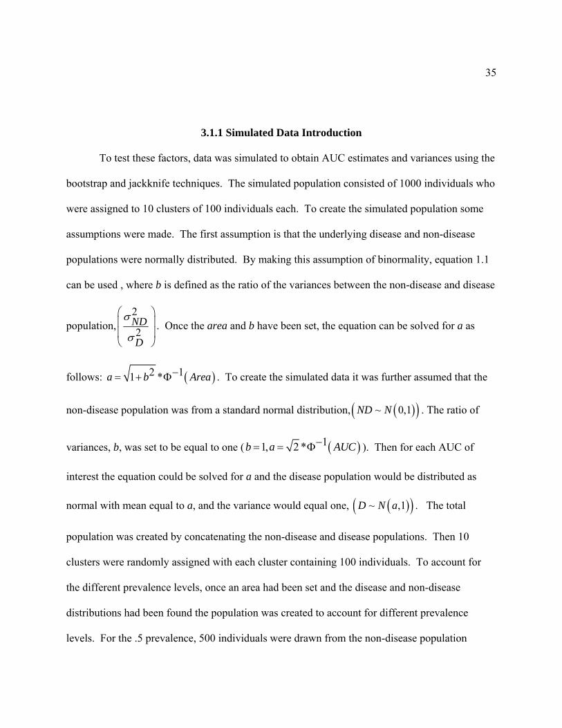
3.1.1 Simulated Data Introduction

To test these factors, data was simulated to obtain AUC estimates and variances using the

bootstrap and jackknife techniques. The simulated population consisted of 1000 individuals who

were assigned to 10 clusters of 100 individuals each. To create the simulated population some

assumptions were made. The first assumption is that the underlying disease and non-disease

populations were normally distributed. By making this assumption of binormality, equation 1.1

can be used , where b is defined as the ratio of the variances between the non-disease and disease

population,2

2ND

D

σ

σ

⎛ ⎞⎜ ⎟⎜ ⎟⎝ ⎠

. Once the area and b have been set, the equation can be solved for a as

follows: ( )2 11 *a b Area−= + Φ . To create the simulated data it was further assumed that the

non-disease population was from a standard normal distribution, )(( )~ 0,1ND N . The ratio of

variances, b, was set to be equal to one ( ( )11, 2 *b a AUC−= = Φ ). Then for each AUC of

interest the equation could be solved for a and the disease population would be distributed as

normal with mean equal to a, and the variance would equal one, )(( )~ ,1D N a . The total

population was created by concatenating the non-disease and disease populations. Then 10

clusters were randomly assigned with each cluster containing 100 individuals. To account for

the different prevalence levels, once an area had been set and the disease and non-disease

distributions had been found the population was created to account for different prevalence

levels. For the .5 prevalence, 500 individuals were drawn from the non-disease population

36 

 

distribution and 500 individuals were drawn from the disease population distribution. For the .3

prevalence, 700 individuals were drawn from the non-disease population distribution and 300

individuals were drawn using the disease population distribution. Finally for the .1 prevalence,

900 individuals were simulated from the non-disease population distribution and 100 individuals

were simulated using the disease population distribution. While the population reflected the

prevalence the 10 clusters were drawn randomly and may not have the same prevalence within

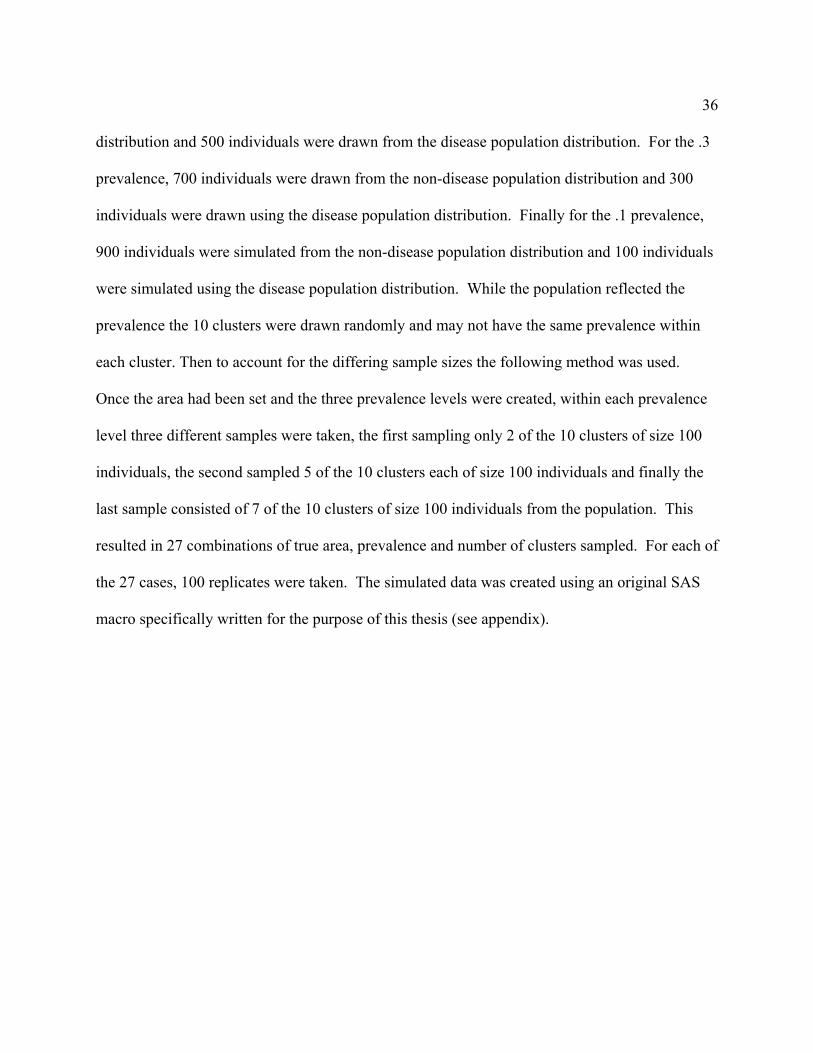
each cluster. Then to account for the differing sample sizes the following method was used.

Once the area had been set and the three prevalence levels were created, within each prevalence

level three different samples were taken, the first sampling only 2 of the 10 clusters of size 100

individuals, the second sampled 5 of the 10 clusters each of size 100 individuals and finally the

last sample consisted of 7 of the 10 clusters of size 100 individuals from the population. This

resulted in 27 combinations of true area, prevalence and number of clusters sampled. For each of

the 27 cases, 100 replicates were taken. The simulated data was created using an original SAS

macro specifically written for the purpose of this thesis (see appendix).

37 

 

3.1.2 Simulated Data: Methods

A previous section detailed how each sample was created for the simulated data. This

section will detail how the bootstrap and jackknife techniques were applied. For a given case,

once a replicate was created it was uploaded into a SAS macro that would determine the AUC

estimate and its variance based on either the jackknife or bootstrap method. A description of the

two original macros designed to analyze the simulated data will now be provided.

In a previous section a general description of the bootstrap method to variance estimation

was given. An original SAS macro was created to carry out this process for the simulated data

created (see appendix). This macro requires the user to specify: an input data set, a total sample

size, the number of bootstrap replicates (B), an index variable and the cluster variable name.

From literature research it was determined to use B =800 bootstrap replicates. Each of the 100

samples within a case simulated as described previously will be used as an input dataset. The

total sample size will be dependent on the number of clusters sampled in the simulated sample,

for 2 clusters sampled the sample size will be 200, for 5 clusters sampled the sample size will be

500 and for 7 clusters sampled the sample size will be 700. For each bootstrap replicate a

pseudo dataset is created by taking a simple random sample with replacement from the original

simulated sample. This pseudo dataset will have the same total sample size as the original

simulated sample; since the sample was taken with replacement certain observations can be

chosen more than once for inclusion in the pseudo dataset. A survey logistic regression is

applied to the pseudo dataset to predict whether or not each observation is from the diseased or

non-diseased population. From the survey logistic regression an AUC estimate is obtained. This

38 

 

process is repeated for B=800 bootstrap replicates on each sample. A dataset is created that

contains the 800 AUC estimates obtained from the 800 bootstrap replicates. The AUC estimate

for the simulated replicate is then determined to be the mean of the 800 replicate AUC estimates.

And the variance for the AUC of the simulated sample is calculated as the variance of the 800

AUC estimates obtained from the 800 bootstrap replicates. This process is done for each of the

100 replicates for each of the 27 cases, so that in the end there are 100 AUC estimates and

variance estimates using the bootstrap technique for each case. Once the 100 replicates for each

case were created the mean AUC and mean variance were computed for each of the 27 cases

from their 100 replicates.

In a previous section a general description of the jackknife method to variance estimation

was given. An original SAS macro was created to carry out this process for the simulated data

created. (See appendix). The macro requires the user to specify: an input data set, a total sample

size, the number of clusters sampled, the sample size within each cluster, an index variable, the

cluster variable name, an individual weight variable and a jackknife weight variable. Again,

total sample size is dependent on the number of clusters sampled and is the same as given above.

The number of clusters sampled will be 2, 5, or 7. The sample size within each cluster is the

same for all samples, 100 individuals in each cluster. The individual weights are calculated as

( )where the total # of clusters in the population = 10 , and M M ss = = # of clusters sampled (2,

5 or 7), giving the following weights: for 2 clusters sampled the weight will be 5, for 5 clusters

sampled the weight will be 2 and for 7 clusters sampled the weight will be approximately 1.4.

The jackknife weight is calculated

39 

 

as 1 where # clusters sampled(2, 5, or 7), cluster sample size = 1001

s nh s nhnhh

−= =

=∑ . So for 2

clusters sampled, the jackknife weight is 1.98, for 5 clusters sampled the jackknife weight is

4.95, and for 7 clusters sampled the jackknife weight is 6.93. For each replicate of each case the

macro first runs a survey logistic regression on the replicate to predict whether each individual

was from the disease or non-disease population. An AUC estimate is obtained from the survey

logistic regression; this will be called the full AUC. A pseudo dataset is then created by

removing one observation from the original replicate dataset. Once an observation is removed

the macro determines from which cluster the observation was taken and reweights the remaining

individuals within that cluster by a factor of 1

nhnh −

where hn is the number of individuals in each

cluster ( )100nh = . The weights of the individuals in the other clusters remain the same. Once

the pseudo dataset is created a survey logistic regression is run to predict whether individuals are

from the disease or non-disease population. From the survey logistic regression an estimate of

the AUC is obtained. This process is repeated until each observation has been removed. Again a

dataset is created that contains the AUC estimates obtained from removing each observation one

at a time. This dataset will be the same size as the original replicate dataset. Again the estimate

for the AUC of the replicate is determined to be the mean of the AUCs from the pseudo datasets.

The variance is then determined to be ( )( )21

1 1

s nnh F inhh iθ θ

⎛ ⎞−−⎜ ⎟

⎝ ⎠= =∑ ∑ where 1

1

s nhnhh

−

=∑ is the

jackknife weight previously calculated and Fθ is the full AUC estimate and ( )iθ is the AUC

estimate from the pseudo dataset where the ith observation was removed and n is the total sample

40 

 

size. This process is done for each replicate, so that in the end there are 100 AUC estimates and

variance estimates using the jackknife technique for each of the 27 cases. Once the 100

replicates for each are obtained the mean AUC and mean variance are computed for each of the

27 cases. The following section will describe the results obtained from these analyses.

41 

 

3.1.3 Simulated Data Results

The true interest lies in determining whether the bootstrap or jackknife techniques for

variance estimation provide better estimates for the AUC. In statistics an estimator is assessed

based on several characteristics. These methods of assessment incorporate a trade-off between

bias and variance of estimators. Bias is defined as the difference between the expected value of

an estimator and the true value of the parameter it is estimating. An estimate is said to be

unbiased if its expected value is equal to the parameter it is estimating. So before we can

compare the variances of the bootstrap and jackknife estimates of AUC we must compare the

estimates themselves to determine if one technique provides estimates that are more biased than

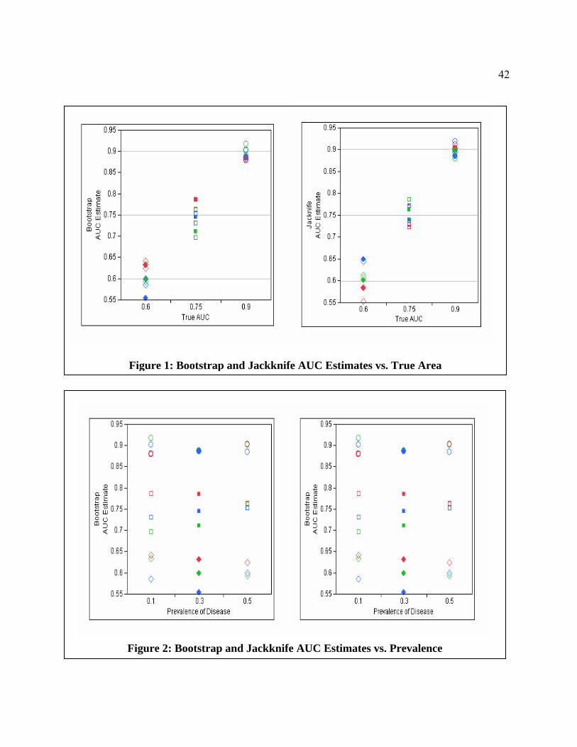
the other. Figure 1 below shows the AUC estimates from each method (Bootstrap and Jackknife)

plotted against the true AUC. As can be seen both methods give consistent results, both methods

provide no bias when estimating the true AUC. Statistical tests confirmed that both the bootstrap

and jackknife AUC estimates were unbiased and that the bootstrap AUC estimates were not

significantly different than the jackknife AUC estimates. Also note in Figure 2 below that the

prevalence of disease does not seem to have any effect on the AUC estimates from either

method.

42 

 

 

Figure 1: Bootstrap and Jackknife AUC Estimates vs. True Area

Figure 2: Bootstrap and Jackknife AUC Estimates vs. Prevalence

43 

 

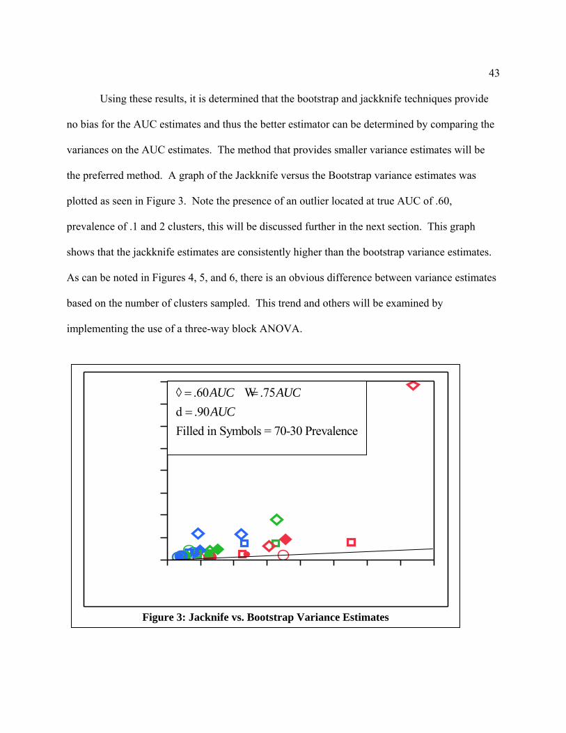
Figure 3: Jacknife vs. Bootstrap Variance Estimates

Using these results, it is determined that the bootstrap and jackknife techniques provide

no bias for the AUC estimates and thus the better estimator can be determined by comparing the

variances on the AUC estimates. The method that provides smaller variance estimates will be

the preferred method. A graph of the Jackknife versus the Bootstrap variance estimates was

plotted as seen in Figure 3. Note the presence of an outlier located at true AUC of .60,

prevalence of .1 and 2 clusters, this will be discussed further in the next section. This graph

shows that the jackknife estimates are consistently higher than the bootstrap variance estimates.

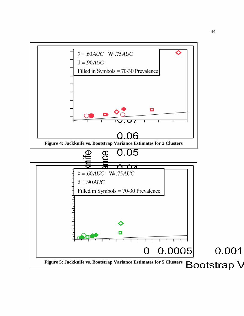
As can be noted in Figures 4, 5, and 6, there is an obvious difference between variance estimates

based on the number of clusters sampled. This trend and others will be examined by

implementing the use of a three-way block ANOVA.

.60 .75

.90 Filled in Symbols = 70-30 Prevalence

AUC AUCAUC

◊ = ==

Wd  

44 

 

 

 

Figure 4: Jackknife vs. Bootstrap Variance Estimates for 2 Clusters

Figure 5: Jackknife vs. Bootstrap Variance Estimates for 5 Clusters

.60 .75

.90 Filled in Symbols = 70-30 Prevalence

AUC AUCAUC

◊ = ==

Wd

.60 .75

.90 Filled in Symbols = 70-30 Prevalence

AUC AUCAUC

◊ = ==

Wd  

45 

 

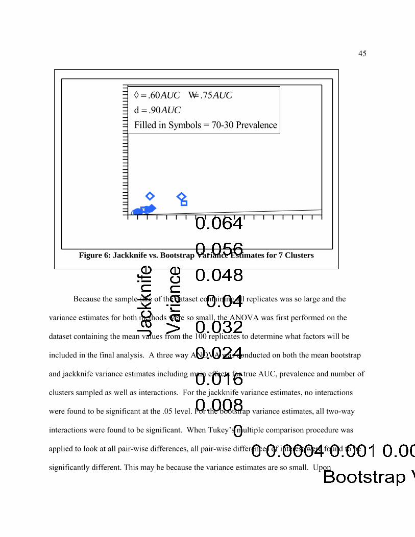
Figure 6: Jackknife vs. Bootstrap Variance Estimates for 7 Clusters

Because the sample size of the dataset containing all replicates was so large and the

variance estimates for both methods were so small, the ANOVA was first performed on the

dataset containing the mean values from the 100 replicates to determine what factors will be

included in the final analysis. A three way ANOVA was conducted on both the mean bootstrap

and jackknife variance estimates including main effects for true AUC, prevalence and number of

clusters sampled as well as interactions. For the jackknife variance estimates, no interactions

were found to be significant at the .05 level. For the bootstrap variance estimates, all two-way

interactions were found to be significant. When Tukey’s multiple comparison procedure was

applied to look at all pair-wise differences, all pair-wise differences of interest were found to be

significantly different. This may be because the variance estimates are so small. Upon

.60 .75

.90 Filled in Symbols = 70-30 Prevalence

AUC AUCAUC

◊ = ==

Wd

46 

 

examining plots of theses two-way interactions, no non-ignorable interactions were found. All

interactions showed similar trends for the different levels of each factor. Therefore it was

decided to omit the two-way interactions in the final analysis. The final analysis performed on

the dataset containing all 100 replicates was a three-way block ANOVA with main effects for

true AUC, prevalence, number of clusters sampled and the block factor of replicate. The results

of the analysis can be found in the Appendix. The block factor consisted of a block for each of

the 100 replicates so that each block contained all 27 cases and there were 100 blocks.

For the bootstrap variance estimates, the ANOVA found that all three characteristics had

an effect on variance estimates. For the true AUC the block ANOVA found, after adjusting for

prevalence level and number of clusters sampled, that area of .90 provided significantly lower

variance estimates than all other areas. Also, area of .75 provided significantly lower variance

estimates than area of .60. Within the prevalence levels the block ANOVA found, after adjusting

for number of clusters sampled and true AUC, that the .1 prevalence level had significantly

higher variance estimates than both the .5 and .3 prevalence levels. Also the .3 prevalence had

significantly higher variance estimates than the .5 prevalence. In other words, as the disease

becomes rarer in the population the variance estimates tend to increase. Finally, within the

different number of clusters sampled the block ANOVA found, after adjusting for prevalence

level and true AUC, that all three cluster groups had significantly different variance estimates.

Two clusters sampled provided the highest variance estimates followed by 5 clusters sampled

and finally 7 clusters sampled provide the smallest variance estimates. In conclusion a three-way

block ANOVA of bootstrap variance estimates including main effects for true AUC, prevalence,

and number of clusters sampled accounting for block factor of replicates, determined that all

47 

 

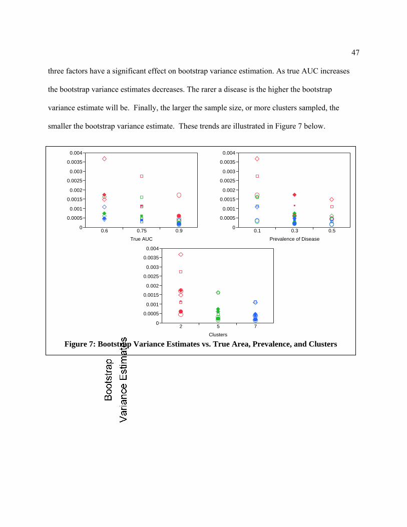
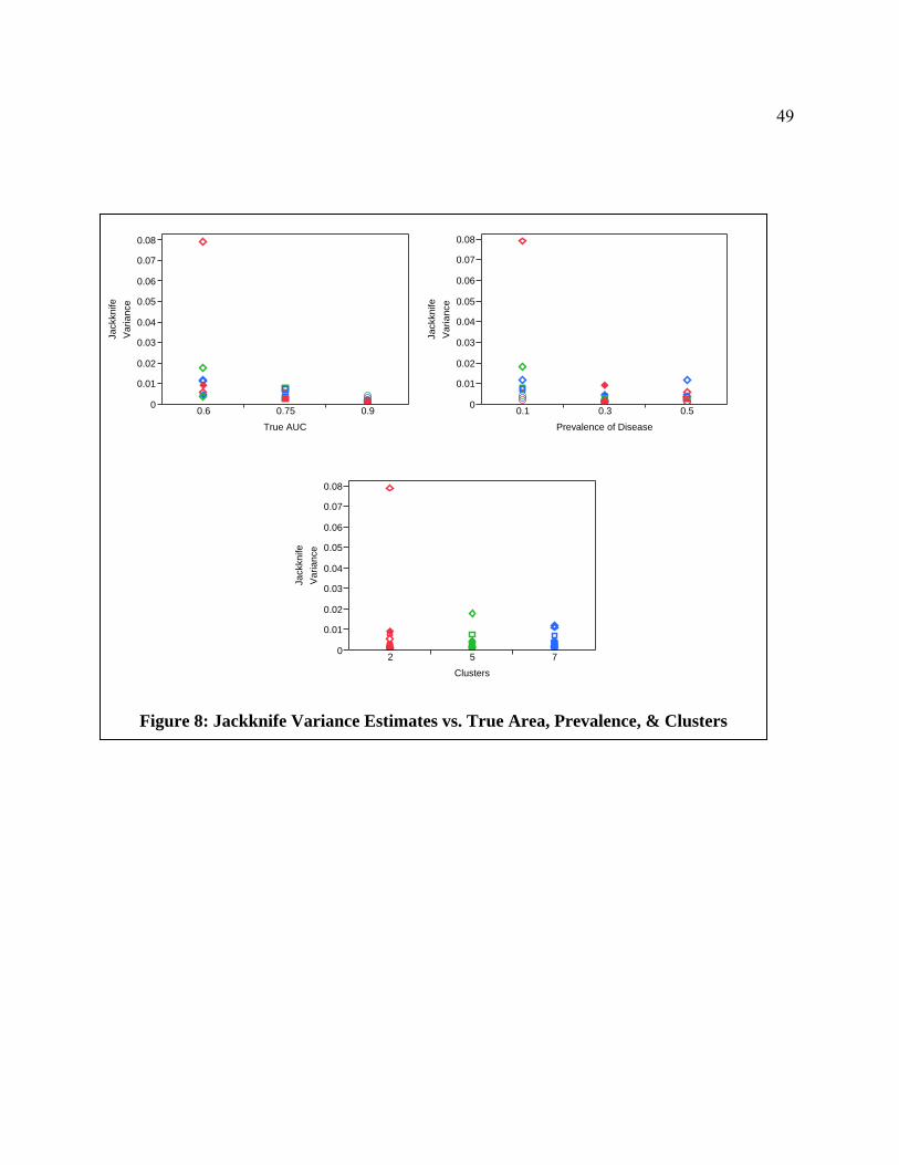
Figure 7: Bootstrap Variance Estimates vs. True Area, Prevalence, and Clusters

three factors have a significant effect on bootstrap variance estimation. As true AUC increases

the bootstrap variance estimates decreases. The rarer a disease is the higher the bootstrap

variance estimate will be. Finally, the larger the sample size, or more clusters sampled, the

smaller the bootstrap variance estimate. These trends are illustrated in Figure 7 below.

0

0.0005

0.001

0.0015

0.002

0.0025

0.003

0.0035

0.004

0.6 0.75 0.9

True AUC

0

0.0005

0.001

0.0015

0.002

0.0025

0.003

0.0035

0.004

0.1 0.3 0.5

Prevalence of Disease

0

0.0005

0.001

0.0015

0.002

0.0025

0.003

0.0035

0.004

2 5 7

Clusters

48 

 

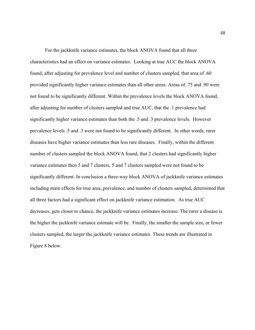
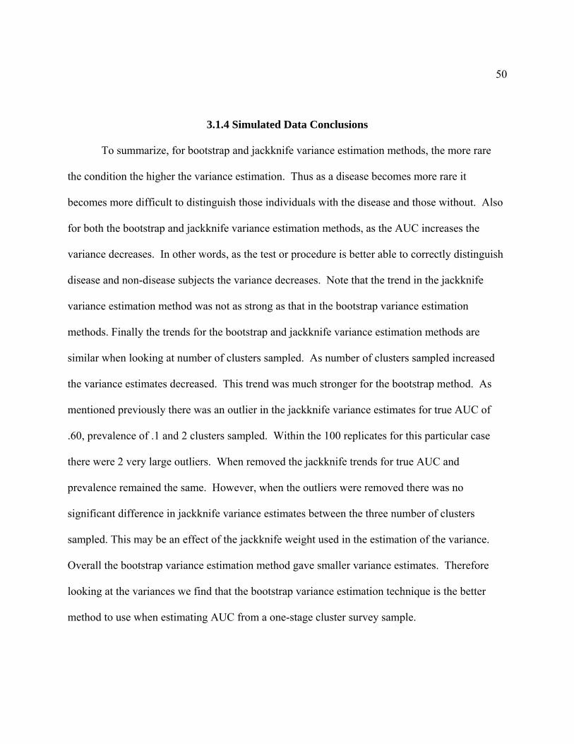
For the jackknife variance estimates, the block ANOVA found that all three

characteristics had an effect on variance estimates. Looking at true AUC the block ANOVA

found, after adjusting for prevalence level and number of clusters sampled, that area of .60

provided significantly higher variance estimates than all other areas. Areas of .75 and .90 were

not found to be significantly different. Within the prevalence levels the block ANOVA found,

after adjusting for number of clusters sampled and true AUC, that the .1 prevalence had

significantly higher variance estimates than both the .5 and .3 prevalence levels. However

prevalence levels .5 and .3 were not found to be significantly different. In other words, rarer

diseases have higher variance estimates than less rare diseases. Finally, within the different

number of clusters sampled the block ANOVA found, that 2 clusters had significantly higher

variance estimates then 5 and 7 clusters, 5 and 7 clusters sampled were not found to be

significantly different. In conclusion a three-way block ANOVA of jackknife variance estimates

including main effects for true area, prevalence, and number of clusters sampled, determined that

all three factors had a significant effect on jackknife variance estimation. As true AUC

decreases, gets closer to chance, the jackknife variance estimates increase. The rarer a disease is

the higher the jackknife variance estimate will be. Finally, the smaller the sample size, or fewer

clusters sampled, the larger the jackknife variance estimates. These trends are illustrated in

Figure 8 below.

49 

 

Figure 8: Jackknife Variance Estimates vs. True Area, Prevalence, & Clusters

0

0.01

0.02

0.03

0.04

0.05

0.06

0.07

0.08

Jack

knife

Var

ianc

e

0.6 0.75 0.9

True AUC 0

0.01

0.02

0.03

0.04

0.05

0.06

0.07

0.08

Jack

knife

Var

ianc

e

0.1 0.3 0.5

Prevalence of Disease

0

0.01

0.02

0.03

0.04

0.05

0.06

0.07

0.08

Jack

knife

Var

ianc

e

2 5 7

Clusters

50 

 

3.1.4 Simulated Data Conclusions

To summarize, for bootstrap and jackknife variance estimation methods, the more rare

the condition the higher the variance estimation. Thus as a disease becomes more rare it

becomes more difficult to distinguish those individuals with the disease and those without. Also

for both the bootstrap and jackknife variance estimation methods, as the AUC increases the

variance decreases. In other words, as the test or procedure is better able to correctly distinguish

disease and non-disease subjects the variance decreases. Note that the trend in the jackknife

variance estimation method was not as strong as that in the bootstrap variance estimation

methods. Finally the trends for the bootstrap and jackknife variance estimation methods are

similar when looking at number of clusters sampled. As number of clusters sampled increased

the variance estimates decreased. This trend was much stronger for the bootstrap method. As

mentioned previously there was an outlier in the jackknife variance estimates for true AUC of

.60, prevalence of .1 and 2 clusters sampled. Within the 100 replicates for this particular case

there were 2 very large outliers. When removed the jackknife trends for true AUC and

prevalence remained the same. However, when the outliers were removed there was no

significant difference in jackknife variance estimates between the three number of clusters

sampled. This may be an effect of the jackknife weight used in the estimation of the variance.

Overall the bootstrap variance estimation method gave smaller variance estimates. Therefore

looking at the variances we find that the bootstrap variance estimation technique is the better

method to use when estimating AUC from a one-stage cluster survey sample.

51 

 

3.2 NHANES Data

The purpose of the NHANES study in this research was to predict whether or not four

hormones have abnormally high levels based on exposure to 10 furans collected from blood

specimens while accounting for menopause status in women sampled to be representative of the

non-institutionalized US population.

3.2.1 NHANES Data Introduction

The National Health and Nutrition Examination Survey (NHANES) as described in a

previous section is unique in that it consists of two parts, interviews and a physical examination.

The interview section involves a questionnaire to obtain demographic information as well as

questions about people’s health and nutrition habits. The physical examination involves the

collection of blood, urine and swab specimens. This section outlines the process for laboratory

collection and the variables of interest for this research.

Blood specimens were collected at the MECs. The blood collection process involved the

use of a screening questionnaire to detect any conditions that may exclude participants from

having their blood drawn. However, the urine collection procedure does not consist of a

questionnaire; it is not as physically demanding. Along with the urine specimen collection,

pregnancy testing was conducted.

Venipuncture, drawn from the examinee’s arm, was used for the blood specimen

collection and the following exclusion criteria were in place for the safety of those patients

unable to safely under blood specimen collection:

52 

 

Hemophiliacs, participants who received chemotherapy within the last 4 weeks, and the

presence of rashes, gauze dressings, casts, edema, paralysis, tubes, open sores or wounds,

withered arms or limbs missing, damaged, sclerosed or occluded veins, allergies to cleansing

reagents, burned or scarred tissue, shunt or intravenous lines on both arms.

According to NHANES, venipuncture is performed to obtain laboratory results that

provide prevalence estimates of disease, risk factors for exam components, and baseline

information on health and nutritional status of the population. The volume of blood drawn

depends on the examinees age. Volume of blood ranges from 9ml for 1-2 years old to 89-92ml

for examinees 12 and older.

In addition to blood specimens, urine is collected to obtain laboratory results that provide

prevalence estimates of disease, risk factors for exam components, and baseline information on

health and nutritional status of the population. No exclusion criteria exist for the collection of

urine specimens. However, urine specimens are only collected on examinees age six and older.

All specimen collection is conducted at the MECs, however only the complete blood

count and pregnancy analyses are performed in the MEC laboratory, the rest of the specimen

analyses are conducted off-site. Training and quality control procedure are in place to ensure the

quality of the laboratory work. There are specific data processing guidelines provided to the

National Center for Health Statistics (NCHS) and contractor staff with standards for naming

variables, filling missing values, and handling missing records. For example, when handling

laboratory results below the lower detection limit they are to be replaced with a value equal to

53 

 

the detection limit divided by the square root of two. The following section will detail the

variables of interest from the laboratory dataset used in this research.

It is of interest to analyze four particular hormones in women. Included are reproductive

hormones, consisting of follicle stimulating hormone (FSH), and luteinizing hormone (LH), and

thyroid hormones, consisting of thyroid stimulating hormone (TSH), and thyroxin (T4).

Menopause status in women can often have a large effect on the levels of these hormones in the

body, and as such, serum FSH and LH levels along with questionnaire data on menstrual history

were used to classify women according to menopausal status. Women were classified as pre-

menopause and post-menopause. Serum FSH and LH along with menopause status are important

for evaluating women’s risk for certain health condition such as cardiovascular disease and

osteoporosis. According to the CDC, serum TSH and T4 levels were used to assess thyroid

function and provide population based reference information on these hormone levels. The

levels of these hormones were classified as being in a normal range or being abnormally high.

The values considered to be abnormally high for each hormone was dependent on menopause

status and differed for each hormone. For FSH a patient, pre-menopause was considered to have

abnormally high levels if the value of FSH was greater than 20, for post-menopause an abnormal

level was greater than 120 (Essig, Follicle Stimulating Hormone). For LH an abnormal level for

pre-menopausal women was an LH value greater than 20, for post-menopausal women abnormal

levels were defined as being greater than 55 (Essig, Luteinizing Hormone). For TSH a pre or

post-menopausal patient was considered to have abnormally high levels if TSH was greater than

4 (Davis). Similarly for T4 a pre or post-menopausal woman was considered to have abnormal

levels if T4 was greater than 12 (Rea).

54 

 

These hormone levels were obtained from the venipuncture collection with .5 milliliters

of blood required to test FSH and LH and 1 milliliter required to test TSH and T4. Only women

age 35 to 60 were eligible to be tested for FSH and LH while all women age 12 and older were

eligible to be tested for TSH and T4. The furans of interest were also obtained from the

venipuncture collection with 4 milliliters of blood being required to test for all ten furans.

Women age 12 and older were eligible to have furan levels tested.

The furans of interest are Tetrachlorodibenzofuran (tcdf), Pentachlorodibenzofuran

(pncdf), Hexachlorodibenzofuran (hxcdf), Heptachlorodibenzofuran (hpcdf), and

Octachlorodibenzofuran (ocdf). From these furans a total of ten measurements were obtained for

use in the analysis. These are 2,3,7,8-tcdf, 1,2,3,7,8-pncdf, 2,3,4,7,8-pncdf, 1,2,3,4,7,8-hcxdf,

1,2,3,6,7,8-hxcdf, 1,2,3,7,8,9-hxcdf, 2,3,4,6,7,8-hxcdf, 1,2,3,4,6,7,8,-hpcdf, 1,2,3,4,7,8,9-hpcdf,

and 1,2,3,4,6,7,8,9-ocdf. These furans fall into a larger category called organochlorines which

according to the CDC are diverse, synthetic chemicals that are persistent in the environment and

tend to bioaccumulate. The CDC claims that assessment of exposure to persistent

organochlorines in a representative sample of the US population is needed to determine current

prevalence and level of exposure and the potential for human health threat from exposure to

these chemicals. It is hypothesized that exposure to these furans have an effect on the level of

several hormones, in particular on TSH, LH, T4 and FSH.

55 

 

3.2.2 NHANES Methods

The previous sections have detailed the NHANES survey, including how it was

conducted and how the measurements were obtained; this section will detail how the bootstrap

and jackknife variance estimation techniques were applied to the data to obtain AUC estimates

and variance estimates. From the previous simulation it was determined that the bootstrap

technique provided smaller variance estimates. It is now of interest to determine if these results

are consistent when applied to data obtained from a complex survey implementing one-stage

cluster sampling. Also it is of interest to determine if exposures to certain furans lead to

abnormally high hormone levels.

A subset of the NHANES survey conducted from 2001-2002 was used in this analysis.

This subset consisted of data collected from 1041 women. The hormones and furans of interest

are described in previous sections. For simplification of analysis, the sum of the ten furans was

used for the analysis instead of each individual furan. Also as mentioned previously the

menopause status of each woman was collected and will be used in analysis to help determine

cut off values for abnormally high levels of hormones.

The NHANES data is formatted so that each individual in the survey is assigned their

own personal weight and thus each person is considered to be their own cluster. Thus for this

research the data consisted of 1041 clusters each of size one. The prevalence of disease for each

hormone is as follows. For both FSH and LH the prevalence of disease was approximately .02

56 

 

(98% normal and 2% abnormal). For both TSH and T4 the prevalence of disease was

approximately .05 (95% normal and 5% abnormal).

An original SAS macro was created to apply the bootstrap technique of variance

estimation to the NHANES data. This macro is similar to the macro used for the simulated data

with a few modifications. The user must again specify an input data set, a total sample size, the

number of bootstrap replicates (B), and an index variable. Since each person is their own cluster,

the macro does not need the user to specify the number of clusters in the dataset, the user does

need to specify the weight variable. This weight variable is supplied to the user in the original

NHANES dataset. And finally the user must specify the response variable to be used in the

logistic regression analysis. In this case the response variable will be each of the four hormones

of interest (TSH, LH, FSH, and T4). The number of replicates will be set to 800. Similarly to

the simulated data, for each replicate a pseudo dataset is created by taking a simple random

sample with replacement from the original dataset. A survey logistic regression is applied to the

pseudo dataset using the sum of the furans and menopause status to predict abnormally high

levels of the hormone. From the survey logistic regression an AUC estimate in obtained. The

estimate for the AUC and variance estimate is calculated the same as before.

Another original SAS macro was created to apply the jackknife variance estimation

method to the NHANES data. The user must specify an input data set, a total sample size, and

an index variable. Since each person is their own cluster, the macro does not need the user to

specify the number of clusters in the dataset, the user does need to specify the weight variable.

This weight variable is supplied to the user in the original NHANES dataset, also a jackknife

57 

 

weight must be specified, and in this case the jackknife weight will always be equal to .999. And

finally the user must specify the response variable to be used in the logistic regression analysis.

In this case the response variable will be each of the four hormones of interest (TSH, LH, FSH,

and T4). A survey logistic regression is applied to the original dataset using the sum of the

furans and menopause status to predict abnormally high levels of the hormone. An AUC

estimate is obtained from the logistic regression, which will be called the full AUC. A pseudo

dataset is then created by removing one observation from the original dataset. Once an

observation is removed the macro then reweights all other observations in the dataset by a factor

of 1

nn −

where n is the total sample size ( )1041n = , since each individual is their own cluster.

Once the pseudo dataset is created a logistic regression is run to predict abnormally high levels

of hormones from exposure to furans and menopause status. From the logistic regression an

estimate of the AUC is obtained. This process is repeated until each observation has been

removed. The AUC estimate and variance estimate is obtained the same as with the simulated

data. The next section will discuss the results found in these analyses for each of the four

reproductive hormones.

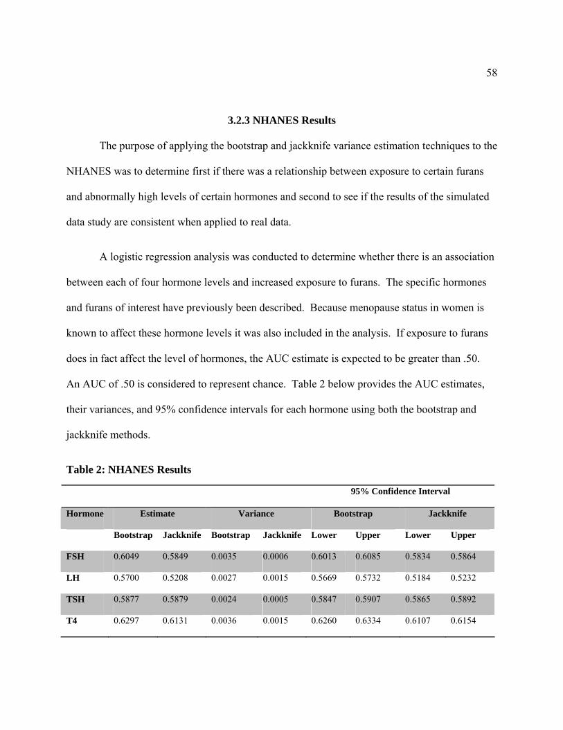
58 

 

3.2.3 NHANES Results

The purpose of applying the bootstrap and jackknife variance estimation techniques to the

NHANES was to determine first if there was a relationship between exposure to certain furans

and abnormally high levels of certain hormones and second to see if the results of the simulated

data study are consistent when applied to real data.

A logistic regression analysis was conducted to determine whether there is an association

between each of four hormone levels and increased exposure to furans. The specific hormones

and furans of interest have previously been described. Because menopause status in women is

known to affect these hormone levels it was also included in the analysis. If exposure to furans

does in fact affect the level of hormones, the AUC estimate is expected to be greater than .50.

An AUC of .50 is considered to represent chance. Table 2 below provides the AUC estimates,

their variances, and 95% confidence intervals for each hormone using both the bootstrap and

jackknife methods.

Table 2: NHANES Results

95% Confidence Interval

Hormone Estimate Variance Bootstrap Jackknife

Bootstrap Jackknife Bootstrap Jackknife Lower Upper Lower Upper

FSH 0.6049 0.5849 0.0035 0.0006 0.6013 0.6085 0.5834 0.5864

LH 0.5700 0.5208 0.0027 0.0015 0.5669 0.5732 0.5184 0.5232

TSH 0.5877 0.5879 0.0024 0.0005 0.5847 0.5907 0.5865 0.5892

T4 0.6297 0.6131 0.0036 0.0015 0.6260 0.6334 0.6107 0.6154

59 

 

As can be seen in Table 2, a logistic regression of FSH and exposure to furans, adjusting

for menopause status yields an AUC estimate higher than 0.5 using both the jackknife and

bootstrap techniques. The bootstrap technique provided an AUC estimate of .605 with a 95%

confidence interval from .601 to .608. The jackknife technique provided an AUC estimate of

.585 with a 95% confidence interval from .583 to .586. These results would seem to suggest that

exposure to certain furans is helpful in predicting abnormally high levels of FSH when

controlling for menopause status.

A logistic regression of LH and exposure to furans, adjusting for menopause status yields

an AUC estimate higher than 0.5 using both the bootstrap and jackknife techniques. The

bootstrap technique provided an AUC estimate of .57 with a 95% confidence interval ranging

from .567 to .573. The jackknife technique provided an AUC estimate of .521 with a 95%

confidence interval ranging from .518 to .523. Although these results are statistically significant

it is unclear whether they are clinically significant.

For TSH, the logistic regression provided an AUC greater than 0.5 for both methods.

The bootstrap method provided an AUC estimate of .588 with a 95% confidence interval from

.585 to .591. The jackknife technique provided an AUC estimate of .588 as well with a 95%

confidence interval from .587 to .589. These results would seem to suggest that exposure to

certain furans is helpful in predicting abnormally high levels of TSH when controlling for

menopause status.

Finally for T4, the logistic regression again provided AUC estimates greater than 0.5 for

both the bootstrap and jackknife techniques. The bootstrap technique provided an AUC estimate

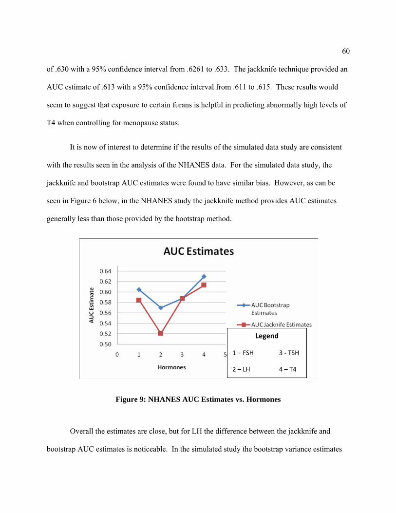
60 

 

of .630 with a 95% confidence interval from .6261 to .633. The jackknife technique provided an

AUC estimate of .613 with a 95% confidence interval from .611 to .615. These results would

seem to suggest that exposure to certain furans is helpful in predicting abnormally high levels of

T4 when controlling for menopause status.

It is now of interest to determine if the results of the simulated data study are consistent

with the results seen in the analysis of the NHANES data. For the simulated data study, the

jackknife and bootstrap AUC estimates were found to have similar bias. However, as can be

seen in Figure 6 below, in the NHANES study the jackknife method provides AUC estimates

generally less than those provided by the bootstrap method.

Figure 9: NHANES AUC Estimates vs. Hormones

 

Overall the estimates are close, but for LH the difference between the jackknife and

bootstrap AUC estimates is noticeable. In the simulated study the bootstrap variance estimates

Legend 

1 – FSH   3 ‐ TSH 

2 – LH    4 – T4 

61 

 

were found to be consistently less than those provided by the jackknife variance estimation

technique. When examining the variance estimates of the NHANES study, the jackknife

variances are consistently smaller than the bootstrap variances. This may be a result of the

jackknife weights. Since each person served as their own cluster in the NHANES study the

jackknife weight was essentially equal to one. In contrast the jackknife weight in the simulated

study ranged from almost 2 to almost 7. This may explain the differences between the two

studies. In summary, with the exception of LH, both the bootstrap and jackknife methods

provided similar AUC estimates for each hormone with jackknife providing smaller variance

estimates.

62 

 

3.2.4 NHANES Conclusions

In conclusion, AUC estimates for all four hormones would suggest that exposure to

furans affect abnormal levels of hormones more than expected by chance. It appears that

exposure to furans does indeed have an effect on hormones in women. This result would suggest

that the US population is being exposed to harmful chemicals in the environment that may be

affecting hormone levels. According to the results the ten furans proved to be most predictive

when predicting abnormally high levels of T4, while adjusting for menopause status in women.

This may suggest that these furans have an impact on T4 hormone levels and may lead to

metabolic health issues in women.

 

63

4 Discussion and Future Work

In comparison of the jackknife and bootstrap variance estimation techniques, the

simulated data study would suggest that the bootstrap technique provides better variance

estimates when working with one stage cluster sample data. However when these

methods were applied to the NHANES study which is structured as a one-stage cluster

sample, the jackknife technique provided smaller variance estimates. Future work in this

area would include further analysis of the jackknife weighting variable used to calculate

the variance. This weight seems to have a great effect on the variance estimates. It

would be of interest to study how these methods compare when equal variance among the

population distributions is not assumed, as was done in the simulated study. Also it

would be of interest to compare the bootstrap and jackknife techniques to the widely used

linearization technique.

Although the results of the two studies seem to disagree, the simulation was able

to explain how certain characteristics of a dataset affect both of these methods. It was

determined that for both methods, bootstrap and jackknife, the rarer a condition is in the

population the higher the variance estimate will be. Also for both techniques as the AUC

estimate increases, the test is doing a better job of correctly predicting the condition, the

variance estimate decreases. Also for the bootstrap, as the number of clusters sampled

increases, variance decreases.

64 

 

Results of the logistic regression analysis of reproductive and thyroid hormones

based on exposure to furans found evidence that the US population’s exposure to

chemicals in its environment may be leading to abnormally high hormone levels. This

result was most strong when looking at Thyroxine. Future work in this area would

include expanding the analysis of these furans and other harmful chemicals to include

children and men. Also it may be of interest in the future to explore other furans and

chemicals present in the environment for their effect on reproductive and thyroid

hormones, as well as other hormone levels not considered here.

65 

 

Bibliography

66 

 

 

 

Bibliography  

 

Booth, Somnath Sarkar and James G. "Monte Carlo Approximation of Bootstrap Variances." The American Statistician (1998): 354‐357. 

Davis, Bets. "Thyroid‐Stimulating Hormone." 11 June 2008. WebMD. 2009 <http://www.webmd.com/a‐to‐z‐guides/thyroid‐stimulating‐hormone‐tsh?page=2>. 

Efron, Robert J. Tibshirani and Bradley. An Introduction to the Bootstrap. New York: Chapman & Hall, 1993. 

Essig, Maria G. "Follicle Stimulating Hormone." 6 June 2007. WebMD. 2009 <http://women.webmd.com/follicle‐stimulating‐hormone?page=2>. 

—. "Luteinizing Hormone." 6 June 2007. WebMD. 2009 <http://women.webmd.com/luteinizing‐hormone?page=4>. 

Giulia Bisoffi, Maria Angela Mazzi and Graham Dunn. "Evaluating screening questionnaires using Receiver Operator Characteristic (ROC) curves from two‐phase (double) samples." International Journal of Methods in Psychiatric Research (n.d.): 121‐133. 

Hanley, Barbara J. McNeil and James A. "The Meaning and Use of the Area under a Receiver Operating CHaracteristic (ROC) Curve." Diagnostic Radiology (1982): 29‐36. 

Izrael, David. "Use of the ROC Curve and the Bootstrap in Comparing Weighted Logistic Regression Models." SUGI 27. Cambridge: Abt Associates Inc, n.d. Paper 248‐27: 1‐5. 

Korn, Barry I. Graubard and Edward L. Analysis of Health Surveys. New York: John Wiley & Sons, Inc., 1999. 

Lee, Eun Sul. Analyzing Complex Survey Data. Thousand Oaks: Sage Publications, Inc., 2006. 

Levy, Paul S. Sampling of Populations. New York: John Wiley & Sons, Inc., n.d. 

67 

 

Mukhopadhyay, Pushpal K. "Try, Try Again: Replication‐Based Variance Estimation Methods for Survey Data." SAS Global Forum. Cary: SAS Institute Inc., 2008. Paper 367:1‐16. 

Rao, KF Rust and Jnk. "Variance estimation for complex surveys using replication techniques." Statistical Methods in Medical Research (1996): 283‐310. 

Rea, Caroline. "Thyroid Hormone Tests." 3 December 2007. WebMD. 2009 <http://www.webmd.com/a‐to‐z‐guides/thyroid‐hormone‐tests?page=3>. 

Rust, Keith. "Variance Estimation for Complex Estimators in Sample Surveys." Journal of Official Statistics (1985): 381‐397. 

SAS Institute, Inc. SAS/STAT 9.2 User Guides. Cary: SAS Institute, Inc., 2008. 

Services, US Department of Health and Human. "National Health and Nutrition Examination Survey, 2007‐2008, Overview." 01 2007. CDC. 2009 <www.cdc.gov/nchs>. 

Zhou, Xiao‐Hua. Statistical Methods in Diagnostic Medicine. New York: John Wiley & Sons, Inc., 2002. 

 

68 

 

APPENDIX

Simulation Macro for Bootstrap

 

libname thesis 'E:\Thesis\Simulation'; %include 'E:\Thesis\Simulation\bootstrap macro sim2.sas'; options nonotes; (Mukhopadhyay) /*Sample Size 200*/ data numbers; input cluster; datalines; 1 2 3 4 5 6 7 8 9 10 ; run; data thesis.Final_Bootstrap_200; AUC_Estimate = 0; SE_AUC=0; Var_AUC=0; prevalence=0; number_of_clusters=0; run; %macro simulation(ndpopsize,area,b, numclusters, sampclusters, case);

69 

 

data nd; %do j= 1 %to &ndpopsize; z = rand('normal', 0, 1); c = 0; output; %end; run; data d; cv=quantile('normal',&area); a1 = sqrt(1 + (&b)**2)*cv; sd= 1/&b; mud=a1*sd; %do j= &ndpopsize+1 %to 1000; z = rand('normal',mud, sd); c = 1; output; %end; run; data pop; set nd d; run; proc print data=pop; run; %do m=1 %to 100; proc surveyselect data=pop method=srs n=100 reps=&numclusters out=clusters; run; data clusters; set clusters; cluster = replicate; run; proc sort data=clusters; by cluster; run; proc surveyselect data=numbers method=srs n=&sampclusters out=new; run; proc sort data=new; by cluster;

70 

 

run; data sample; merge clusters(in=a) new(in=b); by cluster; if a and b ; s = &sampclusters; sampwt=&numclusters/&sampclusters; drop replicate cv a1 sd mud; run; data sample_&m; set sample; id=_n_; true_area = &area; run; %boot(data=sample_&m,reps=800,i=i, strata=cluster, n=200); %if &m = 1 %then %do; data variance; set variance_&m; run; %end; %if &m ^= 1 %then %do; proc append base = variance data = variance_&m force; run; %end; %end; data thesis.case_&case; set variance; run; proc univariate data= variance; var meanAUC; output out=Final mean=AUC_Estimate stdmean=SE_AUC; run; data final; set Final; Var_AUC = SE_AUC**2; *true_area = &area; prevalence = &ndpopsize/10;

71 

 

number_of_clusters = &sampclusters; run; %stack(data=final); %mend; %macro stack(data); proc append base = thesis.Final_Bootstrap_200 data = &data force; run; %mend; %simulation(ndpopsize=500,area=.90,b=1,numclusters=10,sampclusters=2, case=1); %simulation(ndpopsize=700,area=.90,b=1,numclusters=10,sampclusters=2, case=2); %simulation(ndpopsize=900,area=.90,b=1,numclusters=10,sampclusters=2, case=3); %simulation(ndpopsize=500,area=.75,b=1,numclusters=10,sampclusters=2, case=4); %simulation(ndpopsize=700,area=.75,b=1,numclusters=10,sampclusters=2, case=5); %simulation(ndpopsize=900,area=.75,b=1,numclusters=10,sampclusters=2, case=6); %simulation(ndpopsize=500,area=.60,b=1,numclusters=10,sampclusters=2, case=7); %simulation(ndpopsize=700,area=.60,b=1,numclusters=10,sampclusters=2, case=8); %simulation(ndpopsize=900,area=.60,b=1,numclusters=10,sampclusters=2, case=9); /*Sample Size 500*/ data numbers; input cluster; datalines; 1 2 3 4 5 6 7 8 9 10 ; run; data thesis.Final_Bootstrap_500; AUC_Estimate = 0; SE_AUC=0; Var_AUC=0;

72 

 

prevalence=0; number_of_clusters=0; run; %macro simulation(ndpopsize,area,b, numclusters, sampclusters, case); data nd; %do j= 1 %to &ndpopsize; z = rand('normal', 0, 1); c = 0; output; %end; run; data d; cv=quantile('normal',&area); a1 = sqrt(1 + (&b)**2)*cv; sd= 1/&b; mud=a1*sd; %do j= &ndpopsize+1 %to 1000; z = rand('normal',mud, sd); c = 1; output; %end; run; data pop; set nd d; run; proc print data=pop; run; %do m=1 %to 100; proc surveyselect data=pop method=srs n=100 reps=&numclusters out=clusters; run; data clusters; set clusters; cluster = replicate; run; proc sort data=clusters; by cluster; run;

73 

 

proc surveyselect data=numbers method=srs n=&sampclusters out=new; run; proc sort data=new; by cluster; run; data sample; merge clusters(in=a) new(in=b); by cluster; if a and b ; s = &sampclusters; sampwt=&numclusters/&sampclusters; drop replicate cv a1 sd mud; run; data sample_&m; set sample; id=_n_; true_area = &area; run; %boot(data=sample_&m,reps=800,i=i, strata=cluster, n=500); %if &m = 1 %then %do; data variance; set variance_&m; run; %end; %if &m ^= 1 %then %do; proc append base = variance data = variance_&m force; run; %end; %end; data thesis.case_&case; set variance; run; proc univariate data= variance; var meanAUC; output out=Final mean=AUC_Estimate stdmean=SE_AUC; run;

74 

 

data final; set Final; Var_AUC = SE_AUC**2; *true_area = &area; prevalence = &ndpopsize/10; number_of_clusters = &sampclusters; run; %stack(data=final); %mend; %macro stack(data); proc append base = thesis.Final_Bootstrap_500 data = &data force; run; %mend; %simulation(ndpopsize=500,area=.90,b=1,numclusters=10,sampclusters=5, case=10); %simulation(ndpopsize=700,area=.90,b=1,numclusters=10,sampclusters=5, case=11); %simulation(ndpopsize=900,area=.90,b=1,numclusters=10,sampclusters=5, case=12); %simulation(ndpopsize=500,area=.75,b=1,numclusters=10,sampclusters=5, case=13); %simulation(ndpopsize=700,area=.75,b=1,numclusters=10,sampclusters=5, case=14); %simulation(ndpopsize=900,area=.75,b=1,numclusters=10,sampclusters=5, case=15); %simulation(ndpopsize=500,area=.60,b=1,numclusters=10,sampclusters=5, case=16); %simulation(ndpopsize=700,area=.60,b=1,numclusters=10,sampclusters=5, case=17); %simulation(ndpopsize=900,area=.60,b=1,numclusters=10,sampclusters=5, case=18); /*Sample Size 700*/ data numbers; input cluster; datalines; 1 2 3 4 5 6 7 8 9 10 ; run;

75 

 

data thesis.Final_Bootstrap_700; AUC_Estimate = 0; SE_AUC=0; Var_AUC=0; prevalence=0; number_of_clusters=0; run; %macro simulation(ndpopsize,area,b, numclusters, sampclusters, case); data nd; %do j= 1 %to &ndpopsize; z = rand('normal', 0, 1); c = 0; output; %end; run; data d; cv=quantile('normal',&area); a1 = sqrt(1 + (&b)**2)*cv; sd= 1/&b; mud=a1*sd; %do j= &ndpopsize+1 %to 1000; z = rand('normal',mud, sd); c = 1; output; %end; run; data pop; set nd d; run; proc print data=pop; run; %do m=1 %to 100; proc surveyselect data=pop method=srs n=100 reps=&numclusters out=clusters; run; data clusters; set clusters; cluster = replicate;

76 

 

run; proc sort data=clusters; by cluster; run; proc surveyselect data=numbers method=srs n=&sampclusters out=new; run; proc sort data=new; by cluster; run; data sample; merge clusters(in=a) new(in=b); by cluster; if a and b ; s = &sampclusters; sampwt=&numclusters/&sampclusters; drop replicate cv a1 sd mud; run; data sample_&m; set sample; id=_n_; true_area = &area; run; %boot(data=sample_&m,reps=800,i=i, strata=cluster, n=700); %if &m = 1 %then %do; data variance; set variance_&m; run; %end; %if &m ^= 1 %then %do; proc append base = variance data = variance_&m force; run; %end; %end; data thesis.case_&case; set variance; run;

77 

 

proc univariate data= variance; var meanAUC; output out=Final mean=AUC_Estimate stdmean=SE_AUC; run; data final; set Final; Var_AUC = SE_AUC**2; *true_area = &area; prevalence = &ndpopsize/10; number_of_clusters = &sampclusters; run; %stack(data=final); %mend; %macro stack(data); proc append base = thesis.Final_Bootstrap_700 data = &data force; run; %mend; %simulation(ndpopsize=500,area=.90,b=1,numclusters=10,sampclusters=7, case=19); %simulation(ndpopsize=700,area=.90,b=1,numclusters=10,sampclusters=7, case=20); %simulation(ndpopsize=900,area=.90,b=1,numclusters=10,sampclusters=7, case=21); %simulation(ndpopsize=500,area=.75,b=1,numclusters=10,sampclusters=7, case=22); %simulation(ndpopsize=700,area=.75,b=1,numclusters=10,sampclusters=7, case=23); %simulation(ndpopsize=900,area=.75,b=1,numclusters=10,sampclusters=7, case=24); %simulation(ndpopsize=500,area=.60,b=1,numclusters=10,sampclusters=7, case=25); %simulation(ndpopsize=700,area=.60,b=1,numclusters=10,sampclusters=7, case=26); %simulation(ndpopsize=900,area=.60,b=1,numclusters=10,sampclusters=7, case=27);

78 

 

Simulation for Jaccknife

libname thesis 'E:\Thesis\Simulation'; %include 'E:\Thesis\Simulation\jacknife_weight_sim2.sas'; options nonotes; /*Sample Size 200*/ data numbers; input cluster; datalines; 1 2 3 4 5 6 7 8 9 10 ; run; data thesis.Final_Jacknife_200; AUC_Estimate = 0; SE_AUC=0; Var_AUC=0; prevalence=0; number_of_clusters=0; run; %macro simulation(ndpopsize,area,b, numclusters, sampclusters, case); data nd; %do j= 1 %to &ndpopsize; z = rand('normal', 0, 1);

79 

 

c = 0; output; %end; run; data d; cv=quantile('normal',&area); a1 = sqrt(1 + (&b)**2)*cv; sd= 1/&b; mud=a1*sd; %do j= &ndpopsize+1 %to 1000; z = rand('normal',mud, sd); c = 1; output; %end; run; data pop; set nd d; run; proc print data=pop; run; %do m=1 %to 100; proc surveyselect data=pop method=srs n=100 reps=&numclusters out=clusters; run; data clusters; set clusters; cluster = replicate; run; proc sort data=clusters; by cluster; run; proc surveyselect data=numbers method=srs n=&sampclusters out=new; run; proc sort data=new; by cluster; run; data sample; merge clusters(in=a) new(in=b); by cluster; if a and b ;

80 

 

s = &sampclusters; sampwt=&numclusters/&sampclusters; drop replicate cv a1 sd mud; run; data sample_&m; set sample; id=_n_; true_area = &area; run; %jacknife_m2(strata = cluster, s = s, id = id, nh=100, totaln=200, data = work.sample_&m, obs=id, weight=sampwt, jack=1.98); %if &m = 1 %then %do; data var; set var_&m; run; %end; %if &m ^= 1 %then %do; proc append base = var data = var_&m force; run; %end; %end; data thesis.jackcase_&case; set var; run; proc univariate data= var; var meanAUC; output out=Final mean=AUC_Estimate stdmean=SE_AUC; run; data final; set Final; Var_AUC = SE_AUC**2; *true_area = &area; prevalence = &ndpopsize/10; number_of_clusters = &sampclusters; run;

81 

 

%stack(data=final); %mend; %macro stack(data); proc append base = thesis.Final_Jacknife_200 data = &data force; run; %mend; %simulation(ndpopsize=500,area=.90,b=1,numclusters=10,sampclusters=2, case=1); %simulation(ndpopsize=700,area=.90,b=1,numclusters=10,sampclusters=2, case=2); %simulation(ndpopsize=900,area=.90,b=1,numclusters=10,sampclusters=2, case=3); %simulation(ndpopsize=500,area=.75,b=1,numclusters=10,sampclusters=2, case=4); %simulation(ndpopsize=700,area=.75,b=1,numclusters=10,sampclusters=2, case=5); %simulation(ndpopsize=900,area=.75,b=1,numclusters=10,sampclusters=2, case=6); %simulation(ndpopsize=500,area=.60,b=1,numclusters=10,sampclusters=2, case=7); %simulation(ndpopsize=700,area=.60,b=1,numclusters=10,sampclusters=2, case=8); %simulation(ndpopsize=900,area=.60,b=1,numclusters=10,sampclusters=2, case=9); /*Sample Size 500*/ data numbers; input cluster; datalines; 1 2 3 4 5 6 7 8 9 10 ; run; data thesis.Final_Jacknife_500; AUC_Estimate = 0; SE_AUC=0; Var_AUC=0; prevalence=0; number_of_clusters=0; run;

82 

 

%macro simulation(ndpopsize,area,b, numclusters, sampclusters, case); data nd; %do j= 1 %to &ndpopsize; z = rand('normal', 0, 1); c = 0; output; %end; run; data d; cv=quantile('normal',&area); a1 = sqrt(1 + (&b)**2)*cv; sd= 1/&b; mud=a1*sd; %do j= &ndpopsize+1 %to 1000; z = rand('normal',mud, sd); c = 1; output; %end; run; data pop; set nd d; run; proc print data=pop; run; %do m=1 %to 100; proc surveyselect data=pop method=srs n=100 reps=&numclusters out=clusters; run; data clusters; set clusters; cluster = replicate; run; proc sort data=clusters; by cluster; run; proc surveyselect data=numbers method=srs n=&sampclusters out=new; run; proc sort data=new;

83 

 

by cluster; run; data sample; merge clusters(in=a) new(in=b); by cluster; if a and b ; s = &sampclusters; sampwt=&numclusters/&sampclusters; drop replicate cv a1 sd mud; run; data sample_&m; set sample; id=_n_; true_area = &area; run; %jacknife_m2(strata = cluster, s = s, id = id, nh=100, totaln=500, data = work.sample_&m, obs=id, weight=sampwt, jack=4.95); %if &m = 1 %then %do; data var; set var_&m; run; %end; %if &m ^= 1 %then %do; proc append base = var data = var_&m force; run; %end; %end; data thesis.jackcase_&case; set var; run; proc univariate data= var; var meanAUC; output out=Final mean=AUC_Estimate stdmean=SE_AUC; run; data final; set Final;

84 

 

Var_AUC = SE_AUC**2; *true_area = &area; prevalence = &ndpopsize/10; number_of_clusters = &sampclusters; run; %stack(data=final); %mend; %macro stack(data); proc append base = thesis.Final_Jacknife_500 data = &data force; run; %mend; %simulation(ndpopsize=500,area=.90,b=1,numclusters=10,sampclusters=5, case=10); %simulation(ndpopsize=700,area=.90,b=1,numclusters=10,sampclusters=5, case=11); %simulation(ndpopsize=900,area=.90,b=1,numclusters=10,sampclusters=5, case=12); %simulation(ndpopsize=500,area=.75,b=1,numclusters=10,sampclusters=5, case=13); %simulation(ndpopsize=700,area=.75,b=1,numclusters=10,sampclusters=5, case=14); %simulation(ndpopsize=900,area=.75,b=1,numclusters=10,sampclusters=5, case=15); %simulation(ndpopsize=500,area=.60,b=1,numclusters=10,sampclusters=5, case=16); %simulation(ndpopsize=700,area=.60,b=1,numclusters=10,sampclusters=5, case=17); %simulation(ndpopsize=900,area=.60,b=1,numclusters=10,sampclusters=5, case=18); /*Sample Size 700*/ data numbers; input cluster; datalines; 1 2 3 4 5 6 7 8 9 10 ; run; data thesis.Final_Jacknife_700;

85 

 

AUC_Estimate = 0; SE_AUC=0; Var_AUC=0; prevalence=0; number_of_clusters=0; run; %macro simulation(ndpopsize,area,b, numclusters, sampclusters, case); data nd; %do j= 1 %to &ndpopsize; z = rand('normal', 0, 1); c = 0; output; %end; run; data d; cv=quantile('normal',&area); a1 = sqrt(1 + (&b)**2)*cv; sd= 1/&b; mud=a1*sd; %do j= &ndpopsize+1 %to 1000; z = rand('normal',mud, sd); c = 1; output; %end; run; data pop; set nd d; run; proc print data=pop; run; %do m=1 %to 100; proc surveyselect data=pop method=srs n=100 reps=&numclusters out=clusters; run; data clusters; set clusters; cluster = replicate; run; proc sort data=clusters;

86 

 

by cluster; run; proc surveyselect data=numbers method=srs n=&sampclusters out=new; run; proc sort data=new; by cluster; run; data sample; merge clusters(in=a) new(in=b); by cluster; if a and b ; s = &sampclusters; sampwt=&numclusters/&sampclusters; drop replicate cv a1 sd mud; run; data sample_&m; set sample; id=_n_; true_area = &area; run; %jacknife_m2(strata = cluster, s = s, id = id, nh=100, totaln=700, data = work.sample_&m, obs=id, weight=sampwt, jack=6.93); %if &m = 1 %then %do; data var; set var_&m; run; %end; %if &m ^= 1 %then %do; proc append base = var data = var_&m force; run; %end; %end; data thesis.jackcase_&case; set var; run; proc univariate data= var;

87 

 

var meanAUC; output out=Final mean=AUC_Estimate stdmean=SE_AUC; run; data final; set Final; Var_AUC = SE_AUC**2; *true_area = &area; prevalence = &ndpopsize/10; number_of_clusters = &sampclusters; run; %stack(data=final); %mend; %macro stack(data); proc append base = thesis.Final_Jacknife_700 data = &data force; run; %mend; %simulation(ndpopsize=500,area=.90,b=1,numclusters=10,sampclusters=7, case=19); %simulation(ndpopsize=700,area=.90,b=1,numclusters=10,sampclusters=7, case=20); %simulation(ndpopsize=900,area=.90,b=1,numclusters=10,sampclusters=7, case=21); %simulation(ndpopsize=500,area=.75,b=1,numclusters=10,sampclusters=7, case=22); %simulation(ndpopsize=700,area=.75,b=1,numclusters=10,sampclusters=7, case=23); %simulation(ndpopsize=900,area=.75,b=1,numclusters=10,sampclusters=7, case=24); %simulation(ndpopsize=500,area=.60,b=1,numclusters=10,sampclusters=7, case=25); %simulation(ndpopsize=700,area=.60,b=1,numclusters=10,sampclusters=7, case=26); %simulation(ndpopsize=900,area=.60,b=1,numclusters=10,sampclusters=7, case=27);

88 

 

Bootstrap Macro for Simulated Data

%macro boot(data, reps, i, strata,n); %do &i = 1 %to &reps %by 1; proc surveyselect data=&data method=urs sampsize=&n seed=&i out=samp&i outhits outseed; proc surveylogistic data=samp&i; model c (descending) = z; output out = outp p=phat; strata &strata; ods output association = assoc&i; run; data _null_; set assoc&i; if label2 = "c" then call symput ("area", cvalue2); run; data bootstrap&i; set assoc&i; AUC = &area; if label2 = "c"; keep AUC; run; %if &i = 1 %then %do; data bootstrap; set bootstrap&i; run; %end; %if &i ^= 1 %then %do; proc append base = bootstrap data = bootstrap&i force; run; %end; %end;

89 

 

proc univariate data = bootstrap; var AUC; output out = variance_&m var=varAUC mean=meanAUC; run; %mend;

90 

 

Jackknife Macro for Simulated Data

%macro jacknife_m2 (strata, s, id, nh, totaln, data, obs, weight, jack); proc surveylogistic data = &data; model c (descending) = z; weight &weight; ods output association = assoc; run; data _null_; set assoc; if label2 = "c" then call symput ("full", cvalue2); run; %do &id = 1 %to &totaln; data clus ; set &data; if id=&id then call symput('cluster',cluster); run; data test; set &data; if (cluster = &cluster and &obs ^= &id) then wt = &weight*(&nh/(&nh-1)); if (cluster ^= &cluster) then wt = &weight; if (&obs = &id and cluster= &cluster) then wt = .; run; proc surveylogistic data = test; model c (descending) = z; weight wt; ods output association = assoc&id; run; data _null_; set assoc&id; if label2 = "c" then call symput("area", cvalue2);

91 

 

run; data jacknife&id; set assoc&id; keep AUC cluster id; AUC = &area; cluster = &cluster; id = &id; if label2 = "c" ; run; %if &id=1 %then %do; Data jacknife; set jacknife&id; run; %end; %if &id ^= 1 %then %do; proc append base = jacknife data= jacknife&id force; run; %end; %end; data diff; set jacknife; diff = (AUC - &full)*(AUC - &full); run; proc univariate data = diff; var diff; output out = varAUC sum=sumdiff; run; proc univariate data = jacknife; var AUC; output out = estAUC mean=meanAUC; run; data varAUC; set varAUC; var=&jack*sumdiff;

92 

 

keep var; run; data estAUC; set estAUC; keep meanAUC; run; data var_&m; merge varAUC estAUC; run; %mend;

93 

 

Jackknife Macro for NHANES Data

libname a 'C:\Documents and Settings\amdunning\My Documents\Thesis'; ods association; %macro jacknife_m2 (id, totaln, data, obs, weight, jack, hormone); proc surveylogistic data = &data; model &hormone (descending) = sum meno; weight &weight; ods output association = assoc; run; data _null_; set assoc; if label2 = "c" then call symput ("full", cvalue2); run; %do &id = 1 %to &totaln; data clus ; set &data; if id=&id then call symput('cluster',cluster); run; data test; set &data; where id ^= &id; wt = &weight*(&totaln/(&totaln-1)); run; proc surveylogistic data = test; model &hormone (descending) = sum meno; weight wt; ods output association = assoc&id; run; data _null_;

94 

 

set assoc&id; if label2 = "c" then call symput("area", cvalue2); run; data jacknife&id; set assoc&id; keep AUC id; AUC = &area; id = &id; if label2 = "c" ; run; %if &id=1 %then %do; data jacknife; set jacknife&id; run; %end; %if &Id ^= 1 %then %do; proc append base = jacknife data= jacknife&id force; run; %end; %end; data diff; set jacknife; diff = (AUC - &full)*(AUC - &full); run; proc univariate data = diff; var diff; output out = varAUC sum=sumdiff; run; proc univariate data = jacknife; var AUC; output out = estAUC mean=meanAUC; run;

95 

 

data varAUC; set varAUC; var = &jack*sumdiff; keep var; run; data estAUC; set estAUC; keep meanAUC; run; data var_&hormone; set varAUC estAUC; run; %mend;

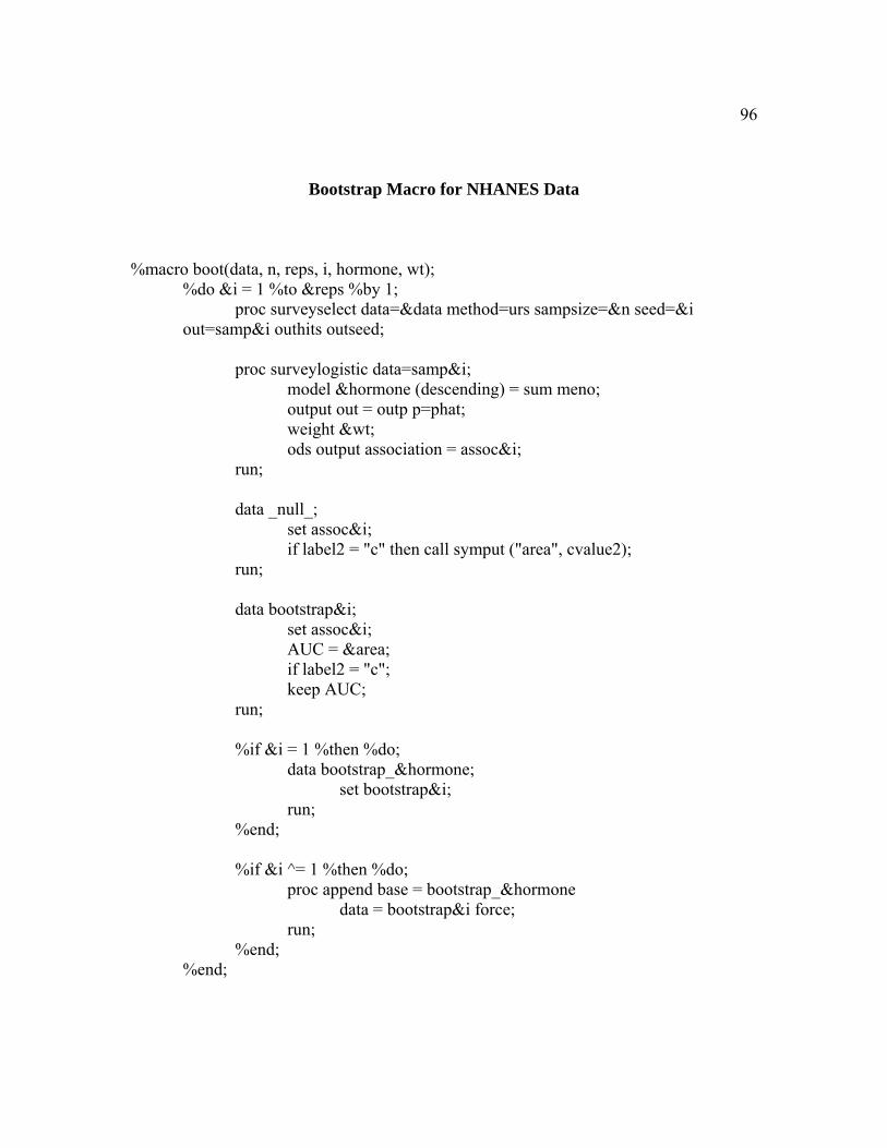
96 

 

Bootstrap Macro for NHANES Data

%macro boot(data, n, reps, i, hormone, wt); %do &i = 1 %to &reps %by 1; proc surveyselect data=&data method=urs sampsize=&n seed=&i out=samp&i outhits outseed; proc surveylogistic data=samp&i; model &hormone (descending) = sum meno; output out = outp p=phat; weight &wt; ods output association = assoc&i; run; data _null_; set assoc&i; if label2 = "c" then call symput ("area", cvalue2); run; data bootstrap&i; set assoc&i; AUC = &area; if label2 = "c"; keep AUC; run; %if &i = 1 %then %do; data bootstrap_&hormone; set bootstrap&i; run; %end; %if &i ^= 1 %then %do; proc append base = bootstrap_&hormone data = bootstrap&i force; run; %end; %end;

97 

 

proc univariate data = bootstrap_&hormone; var AUC; output out = variance_&hormone var=varAUC mean=meanAUC; run; %mend;

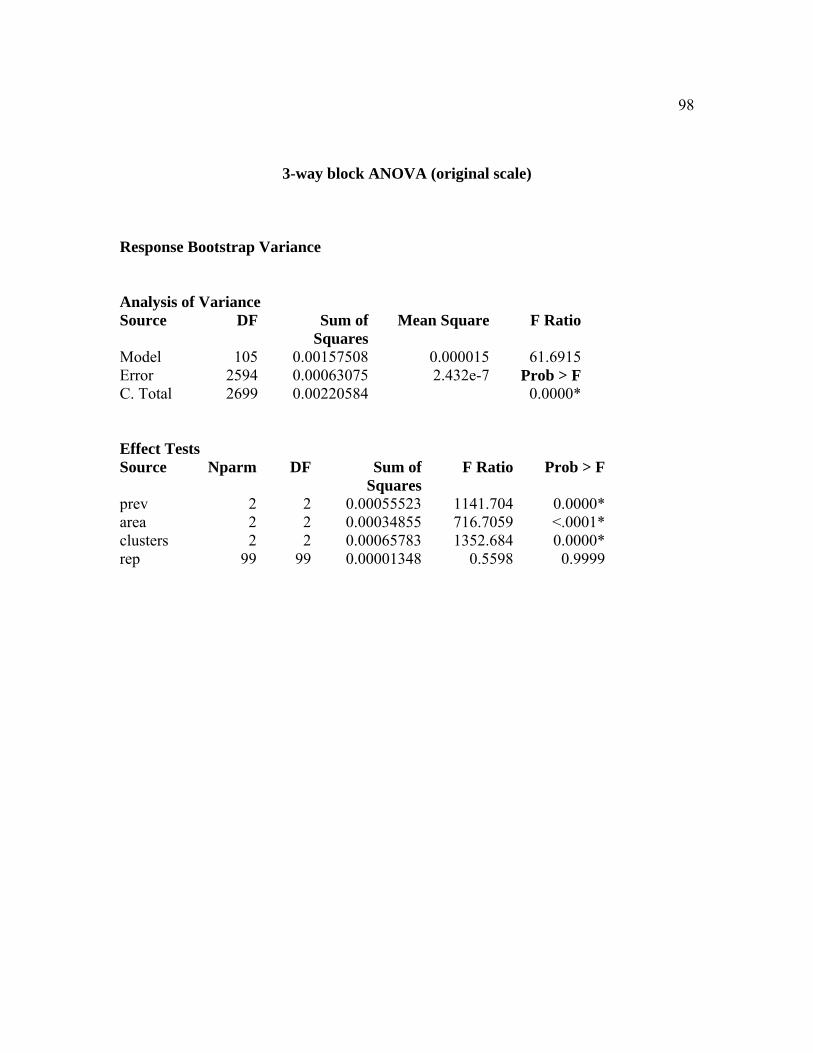
98 

 

3-way block ANOVA (original scale)

Response Bootstrap Variance Analysis of Variance Source DF Sum of

SquaresMean Square F Ratio

Model 105 0.00157508 0.000015 61.6915 Error 2594 0.00063075 2.432e-7 Prob > F C. Total 2699 0.00220584 0.0000* Effect Tests Source Nparm DF Sum of

SquaresF Ratio Prob > F

prev 2 2 0.00055523 1141.704 0.0000* area 2 2 0.00034855 716.7059 <.0001* clusters 2 2 0.00065783 1352.684 0.0000* rep 99 99 0.00001348 0.5598 0.9999

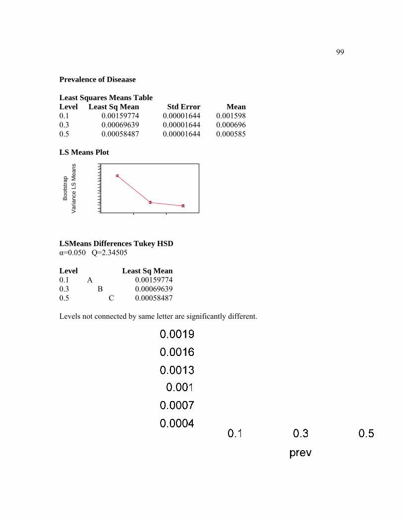
99 

 

Prevalence of Diseaase Least Squares Means Table Level Least Sq Mean Std Error Mean0.1 0.00159774 0.00001644 0.0015980.3 0.00069639 0.00001644 0.0006960.5 0.00058487 0.00001644 0.000585 LS Means Plot

Boo

tstra

pV

aria

nce

LS M

eans

LSMeans Differences Tukey HSD α=0.050 Q=2.34505 Level Least Sq Mean0.1 A 0.001597740.3 B 0.000696390.5 C 0.00058487 Levels not connected by same letter are significantly different.

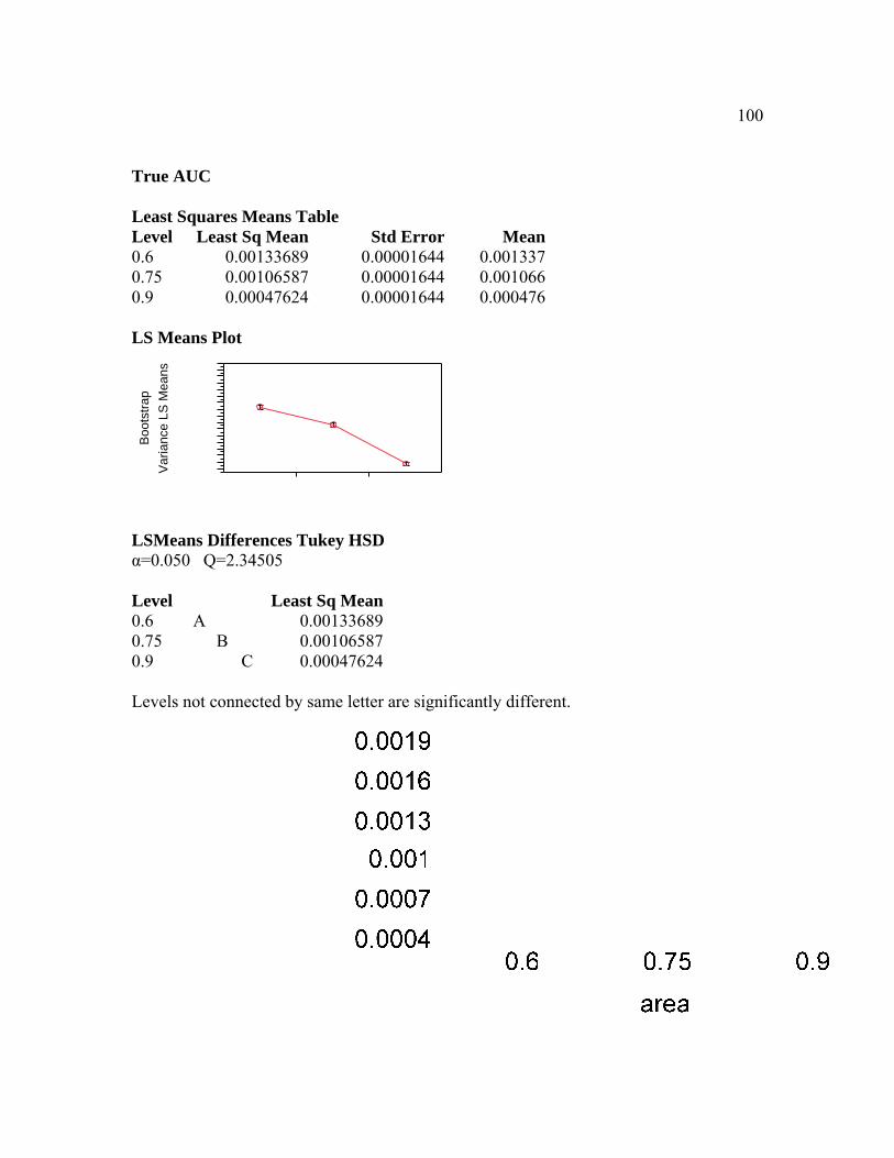
100 

 

True AUC Least Squares Means Table Level Least Sq Mean Std Error Mean0.6 0.00133689 0.00001644 0.0013370.75 0.00106587 0.00001644 0.0010660.9 0.00047624 0.00001644 0.000476 LS Means Plot

Boo

tstra

pV

aria

nce

LS M

eans

LSMeans Differences Tukey HSD α=0.050 Q=2.34505 Level Least Sq Mean0.6 A 0.001336890.75 B 0.001065870.9 C 0.00047624 Levels not connected by same letter are significantly different.

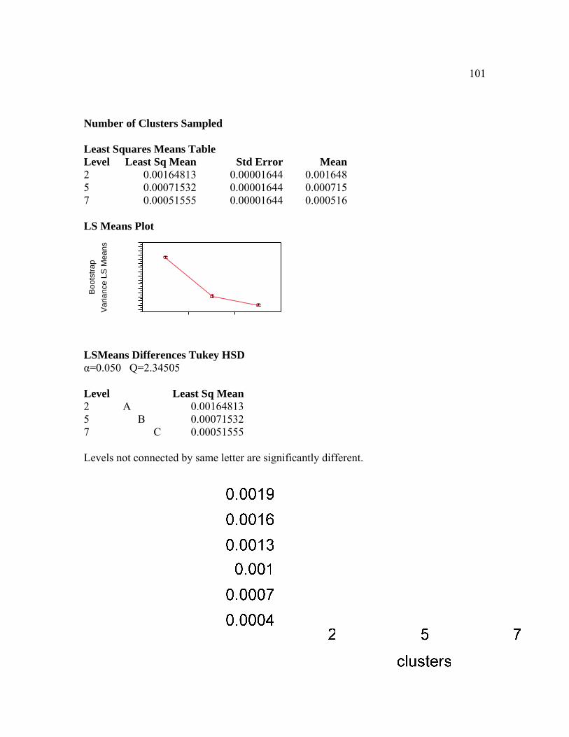
101 

 

Number of Clusters Sampled Least Squares Means Table Level Least Sq Mean Std Error Mean2 0.00164813 0.00001644 0.0016485 0.00071532 0.00001644 0.0007157 0.00051555 0.00001644 0.000516 LS Means Plot

Boo

tstra

pV

aria

nce

LS M

eans

LSMeans Differences Tukey HSD α=0.050 Q=2.34505 Level Least Sq Mean2 A 0.001648135 B 0.000715327 C 0.00051555 Levels not connected by same letter are significantly different.

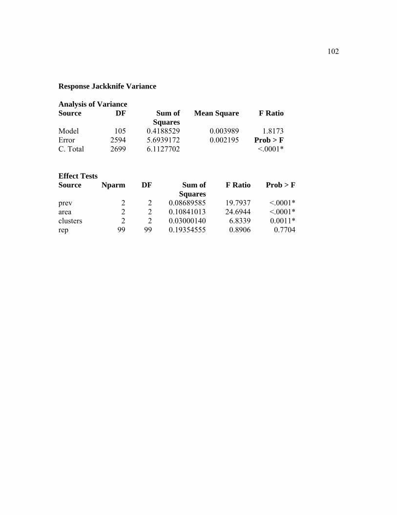
102 

 

Response Jackknife Variance Analysis of Variance Source DF Sum of

SquaresMean Square F Ratio

Model 105 0.4188529 0.003989 1.8173 Error 2594 5.6939172 0.002195 Prob > F C. Total 2699 6.1127702 <.0001* Effect Tests Source Nparm DF Sum of

SquaresF Ratio Prob > F

prev 2 2 0.08689585 19.7937 <.0001* area 2 2 0.10841013 24.6944 <.0001* clusters 2 2 0.03000140 6.8339 0.0011* rep 99 99 0.19354555 0.8906 0.7704

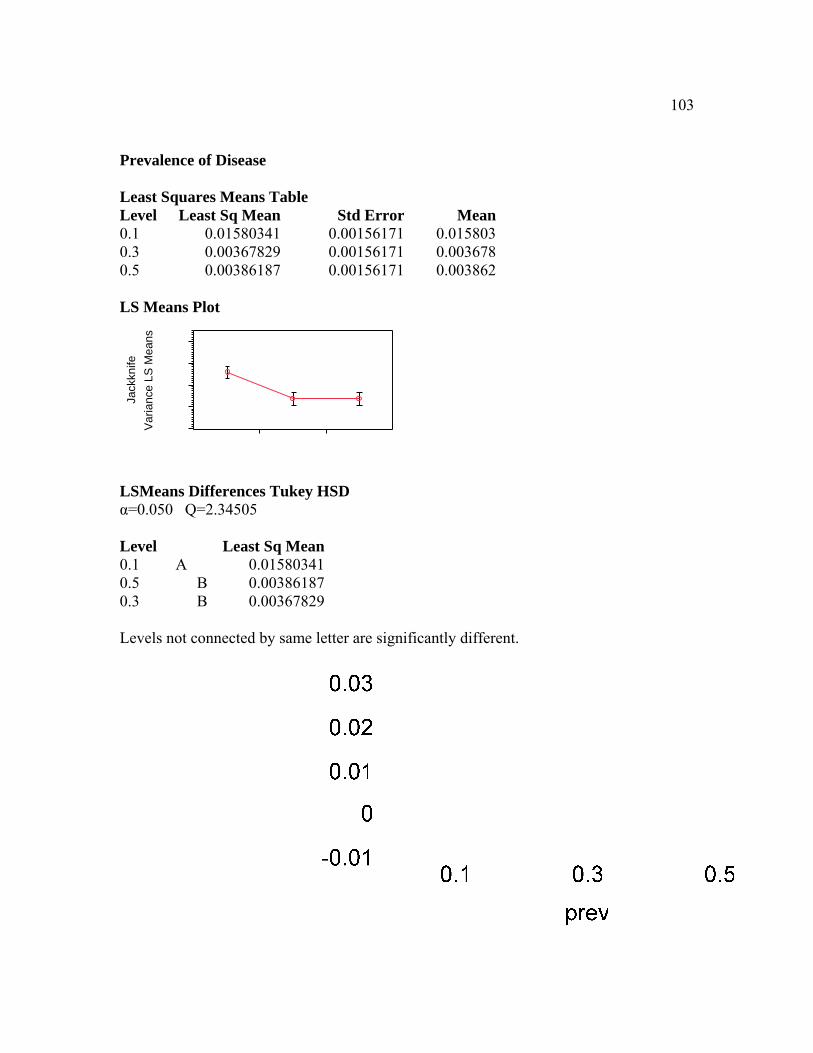
103 

 

Prevalence of Disease Least Squares Means Table Level Least Sq Mean Std Error Mean0.1 0.01580341 0.00156171 0.0158030.3 0.00367829 0.00156171 0.0036780.5 0.00386187 0.00156171 0.003862 LS Means Plot

Jack

knife

Var

ianc

e LS

Mea

ns

LSMeans Differences Tukey HSD α=0.050 Q=2.34505 Level Least Sq Mean 0.1 A 0.01580341 0.5 B 0.00386187 0.3 B 0.00367829 Levels not connected by same letter are significantly different.

104 

 

True AUC Least Squares Means Table Level Least Sq Mean Std Error Mean0.6 0.01661686 0.00156171 0.0166170.75 0.00465798 0.00156171 0.0046580.9 0.00206873 0.00156171 0.002069 LS Means Plot

Jack

knife

Var

ianc

e LS

Mea

ns

LSMeans Differences Tukey HSD α=0.050 Q=2.34505 Level Least Sq Mean 0.6 A 0.01661686 0.75 B 0.00465798 0.9 B 0.00206873 Levels not connected by same letter are significantly different.

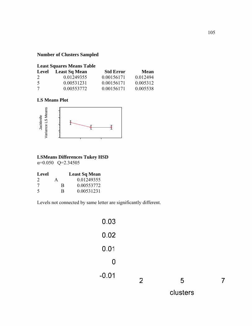
105 

 

Number of Clusters Sampled Least Squares Means Table Level Least Sq Mean Std Error Mean2 0.01249355 0.00156171 0.0124945 0.00531231 0.00156171 0.0053127 0.00553772 0.00156171 0.005538 LS Means Plot

Jack

knife

Var

ianc

e LS

Mea

ns

LSMeans Differences Tukey HSD α=0.050 Q=2.34505 Level Least Sq Mean 2 A 0.01249355 7 B 0.00553772 5 B 0.00531231 Levels not connected by same letter are significantly different.

106 

 

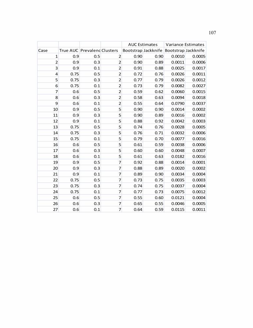
107 

 

Case True AUC Prevalenc Clusters Bootstrap Jackknife Bootstrap Jackknife 1 0.9 0.5 2 0.90 0.90 0.0010 0.00052 0.9 0.3 2 0.90 0.89 0.0011 0.00063 0.9 0.1 2 0.91 0.88 0.0025 0.00174 0.75 0.5 2 0.72 0.76 0.0026 0.00115 0.75 0.3 2 0.77 0.79 0.0026 0.00126 0.75 0.1 2 0.73 0.79 0.0082 0.00277 0.6 0.5 2 0.59 0.62 0.0060 0.00158 0.6 0.3 2 0.58 0.63 0.0094 0.00189 0.6 0.1 2 0.55 0.64 0.0790 0.003710 0.9 0.5 5 0.90 0.90 0.0014 0.000211 0.9 0.3 5 0.90 0.89 0.0016 0.000212 0.9 0.1 5 0.88 0.92 0.0042 0.000313 0.75 0.5 5 0.74 0.76 0.0028 0.000514 0.75 0.3 5 0.76 0.71 0.0032 0.000615 0.75 0.1 5 0.79 0.70 0.0077 0.001616 0.6 0.5 5 0.61 0.59 0.0038 0.000617 0.6 0.3 5 0.60 0.60 0.0048 0.000718 0.6 0.1 5 0.61 0.63 0.0182 0.001619 0.9 0.5 7 0.92 0.88 0.0014 0.000120 0.9 0.3 7 0.88 0.89 0.0020 0.000221 0.9 0.1 7 0.89 0.90 0.0034 0.000422 0.75 0.5 7 0.73 0.75 0.0035 0.000323 0.75 0.3 7 0.74 0.75 0.0037 0.000424 0.75 0.1 7 0.77 0.73 0.0075 0.001225 0.6 0.5 7 0.55 0.60 0.0121 0.000426 0.6 0.3 7 0.65 0.55 0.0046 0.000527 0.6 0.1 7 0.64 0.59 0.0115 0.0011

AUC Estimates Variance Estimates

108 

 

VITA

Allison Marie Dunning was born in Wichita. Kansas, and grew up in Martinsville,

Virginia, where she attended Magna Vista High School. After high school, she went to

Virginia Tech in Blacksburg, Virginia. She graduated with a Bachelor’s of Science

degree in Statistics in May 2007. Allison then moved to Richmond, where she started in

the Biostatistics Department at VCU. She worked as a Graduate Teaching Assistant for

the BIOS 543 and 543 courses from 2007-2009, as well as an Adjunct Instructor with the

Statistics Department teaching labs for the STAT 208 course for 2009. She is currently

looking for employment in the Research Triangle Park in North Carolina.

 

109