LMS J. Comput. Math. 15 (2012) 341–359 Ce2012 Authordoi:10.1112/S1461157012001088

Efficient implementation of theHardy–Ramanujan–Rademacher formula

Fredrik Johansson

Abstract

We describe how the Hardy–Ramanujan–Rademacher formula can be implemented to allow thepartition function p(n) to be computed with softly optimal complexity O(n1/2+o(1)) and verylittle overhead. A new implementation based on these techniques achieves speedups in excess ofa factor 500 over previously published software and has been used by the author to calculatep(1019), an exponent twice as large as in previously reported computations. We also investigateperformance for multi-evaluation of p(n), where our implementation of the Hardy–Ramanujan–Rademacher formula becomes superior to power series methods on far denser sets of indices thanprevious implementations. As an application, we determine over 22 billion new congruences forthe partition function, extending Weaver’s tabulation of 76 065 congruences.

Supplementary materials are available with this article.

1. Introduction

Let p(n) denote the number of partitions of n, or the number of ways that n can be written asa sum of positive integers without regard to the order of the terms [27, A000041]. The classicalway to compute p(n) uses the generating function representation of p(n) combined with Euler’spentagonal number theorem

∞∑n=0

p(n)xn =∞∏k=1

11− xk

=( ∞∑k=−∞

(−1)kxk(3k−1)/2

)−1

(1.1)

from which one can construct the recursive relation

p(n) =n∑k=1

(−1)k+1

(p

(n− k(3k − 1)

2

)+ p

(n− k(3k + 1)

2

)). (1.2)

Equation (1.2) provides a simple and reasonably efficient way to compute the list of valuesp(0), p(1), . . . , p(n− 1), p(n). Alternatively, applying Fast Fourier Transform (FFT)-basedpower series inversion to the right-hand side of (1.1) gives an asymptotically faster, essentiallyoptimal algorithm for the same set of values.

An attractive feature of Euler’s method, in both the recursive and FFT incarnations, is thatthe values can be computed more efficiently modulo a small prime number. This is useful forinvestigating partition function congruences, such as in a recent large-scale computation ofp(n) modulo small primes for n up to 109 (see [7]).

While efficient for computing p(n) for all n up to some limit, Euler’s formula is impracticalfor evaluating p(n) for an isolated, large n. One of the most astonishing number-theoreticaldiscoveries of the 20th century is the Hardy–Ramanujan–Rademacher (HRR) formula, firstgiven as an asymptotic expansion by Hardy and Ramanujan in 1917 [15] and subsequentlyrefined to an exact representation by Rademacher in 1936 [31], which provides a direct andcomputationally efficient expression for the single value p(n).

Received 31 October 2011; revised 1 June 2012.

2010 Mathematics Subject Classification 11Y55 (primary), 11-04, 11P83 (secondary).

Supported by Austrian Science Fund (FWF) grant Y464-N18 (Fast Computer Algebra for Special Functions).

342 F. JOHANSSON

Simplified to a first-order estimate, the HRR formula states that

p(n)∼ 14n√

3eπ√

2n/3, (1.3)

from which one gathers that p(n) is a number with roughly n1/2 decimal digits. The full versioncan be stated as

p(n) =N∑k=1

(√3k

424n− 1

)Ak(n) U

(C(n)k

)+R(n, N), (1.4)

U(x) = cosh(x)− sinh(x)x

, C(n) =π

6√

24n− 1, (1.5)

Ak(n) =k−1∑h=0

δgcd(h,k),1 exp(πi

[s(h, k)− 2hn

k

])(1.6)

where s(h, k) is the Dedekind sum

s(h, k) =k−1∑i=1

i

k

(hi

k−⌊hi

k

⌋− 1

2

)(1.7)

and where the remainder satisfies |R(n, N)|<M(n, N) with

M(n, N) =44π2

225√

3N−1/2 +

π√

275

(N

n− 1

)1/2

sinh

(π

N

√2n3

). (1.8)

It is easily shown that M(n, cn1/2)∼ n−1/4 for every positive c. Rademacher’s bound (1.8)therefore implies that O(n1/2) terms in (1.4) suffice to compute p(n) exactly by forcing|R(n, N)|< 1/2 and rounding to the nearest integer. For example, we can take N = dn1/2ewhen n> 65.

In fact, it was pointed out by Odlyzko [21, 26] that the HRR formula ‘gives an algorithmfor calculating p(n) that is close to optimal, since the number of bit operations is not muchlarger than the number of bits of p(n)’. In other words, the time complexity should not bemuch higher than the trivial lower bound Ω(n1/2) derived from (1.3) just for writing downthe result. Odlyzko’s claim warrants some elaboration, since the HRR formula ostensibly is atriply nested sum containing O(n3/2) inner terms.

The computational utility of the HRR formula was, of course, realized long before theavailability of electronic computers. For instance, Lehmer [23] used it to verify Ramanujan’sconjectures p(599)≡ 0 mod 53 and p(721)≡ 0 mod 112. Implementations are now available innumerous mathematical software systems, including Pari/GP [29], Mathematica [40] andSage [34]. However, apart from Odlyzko’s remark, we find few algorithmic accounts of theHRR formula in the literature, nor any investigation into the optimality of the availableimplementations.

The present paper describes a new C implementation of the HRR formula. The code is freelyavailable as a component of the Fast Library for Number Theory (FLINT) [16], released underthe terms of the GNU General Public License. We show that the complexity for computingp(n) indeed can be bounded by O(n1/2+o(1)), and observe that our implementation comes closeto being optimal in practice, improving on the speed of previously published software by morethan two orders of magnitude.

We benchmark the code by computing some extremely large isolated values of p(n). We alsoinvestigate efficiency compared to power series methods for evaluation of multiple values, andfinally apply our implementation to the problem of computing congruences for p(n).

EFFICIENT IMPLEMENTATION OF THE HRR FORMULA 343

2. Simplification of exponential sums

A naive implementation of formulas (1.4)–(1.7) requires O(n3/2) integer operations to evaluateDedekind sums, and O(n) numerical evaluations of complex exponentials (or cosines, since theimaginary parts ultimately cancel out). In the following section, we describe how the number ofinteger operations and cosine evaluations can be reduced, for the moment ignoring numericalevaluation.

A first improvement, used for instance in the Sage implementation, is to recognize thatDedekind sums can be evaluated in O(log k) steps using a GCD-style algorithm, as describedby Apostol [2], or with Knuth’s fraction-free algorithm [20] which avoids the overhead ofrational arithmetic. This reduces the total number of integer operations to O(n log n), whichis a dramatic improvement but still leaves the cost of computing p(n) quadratic in the size ofthe final result.

Fortunately, the Ak(n) sums have additional structure as discussed in [14, 22, 24, 32, 39],allowing the computational complexity to be reduced. Since numerous implementers of theHRR formula until now appear to have overlooked these results, it seems appropriate that wereproduce the main formulas and assess the computational issues in more detail. We describetwo concrete algorithms: one simple, and one asymptotically fast, the latter being implementedin FLINT.

2.1. A simple algorithm

Using properties of the Dedekind eta function, one can derive the formula (whichWhiteman [39] attributes to Selberg)

Ak(n) =(k

3

)1/2 ∑(3l2+l)/2≡−n mod k

(−1)l cos(

6l + 16k

π

)(2.1)

in which the summation ranges over 0 6 l < 2k and only O(k1/2) terms are nonzero. With asimple brute force search for solutions of the quadratic equation, this representation providesa way to compute Ak(n) that is both simpler and more efficient than the usual definition (1.6).

Although a brute force search requires O(k) loop iterations, the successive quadratic termscan be generated without multiplications or divisions using two coupled linear recurrences.This only costs a few processor cycles per loop iteration, which is a substantial improvementover computing Dedekind sums, and means that the cost up to fairly large k effectively willbe dominated by evaluating O(k1/2) cosines, adding up to O(n3/4) function evaluations forcomputing p(n).

A basic implementation of (2.1) is given as Algorithm 1. Here the variable m runs overthe successive values of (3l2 + l)/2, and r runs over the differences between consecutive m.Various improvements are possible: a modification of the equation allows cutting the looprange in half when k is odd, and the number of cosine evaluations can be reduced by countingthe multiplicities of unique angles after reduction to [0, π/4), evaluating a weighted sum∑wi cos(θi) at the end, possibly using trigonometric addition theorems to exploit the fact

that the differences θi+1 − θi between successive angles tend to repeat for many different i.

2.2. A fast algorithm

From Selberg’s formula (2.1), a still more efficient but considerably more complicatedmultiplicative decomposition of Ak(n) can be obtained. The advantage of this representationis that it only contains O(log k) cosine factors, bringing the total number of cosine evaluationsfor p(n) down to O(n1/2 log n). It also reveals exactly when Ak(n) = 0 (which is about half thetime). We stress that these results are not new; the formulas are given in full detail and withproofs in [39].

344 F. JOHANSSON

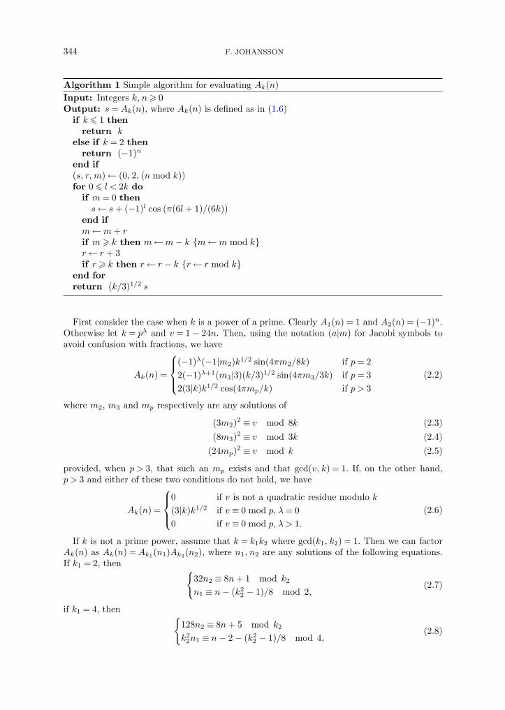
Algorithm 1 Simple algorithm for evaluating Ak(n)Input: Integers k, n> 0Output: s=Ak(n), where Ak(n) is defined as in (1.6)

if k 6 1 thenreturn k

else if k = 2 thenreturn (−1)n

end if(s, r, m)← (0, 2, (n mod k))for 0 6 l < 2k do

if m= 0 thens← s+ (−1)l cos (π(6l + 1)/(6k))

end ifm←m+ rif m> k then m←m− k m←m mod kr← r + 3if r > k then r← r − k r← r mod k

end forreturn (k/3)1/2 s

First consider the case when k is a power of a prime. Clearly A1(n) = 1 and A2(n) = (−1)n.Otherwise let k = pλ and v = 1− 24n. Then, using the notation (a|m) for Jacobi symbols toavoid confusion with fractions, we have

Ak(n) =

(−1)λ(−1|m2)k1/2 sin(4πm2/8k) if p= 22(−1)λ+1(m3|3)(k/3)1/2 sin(4πm3/3k) if p= 32(3|k)k1/2 cos(4πmp/k) if p > 3

(2.2)

where m2, m3 and mp respectively are any solutions of

(3m2)2 ≡ v mod 8k (2.3)

(8m3)2 ≡ v mod 3k (2.4)

(24mp)2 ≡ v mod k (2.5)

provided, when p > 3, that such an mp exists and that gcd(v, k) = 1. If, on the other hand,p > 3 and either of these two conditions do not hold, we have

Ak(n) =

0 if v is not a quadratic residue modulo k(3|k)k1/2 if v ≡ 0 mod p, λ= 00 if v ≡ 0 mod p, λ > 1.

(2.6)

If k is not a prime power, assume that k = k1k2 where gcd(k1, k2) = 1. Then we can factorAk(n) as Ak(n) =Ak1(n1)Ak2(n2), where n1, n2 are any solutions of the following equations.If k1 = 2, then

32n2 ≡ 8n+ 1 mod k2

n1 ≡ n− (k22 − 1)/8 mod 2,

(2.7)

if k1 = 4, then 128n2 ≡ 8n+ 5 mod k2

k22n1 ≡ n− 2− (k2

2 − 1)/8 mod 4,(2.8)

EFFICIENT IMPLEMENTATION OF THE HRR FORMULA 345

and if k1 is odd or divisible by 8, thenk2

2d2en1 ≡ d2en+ (k22 − 1)/d1 mod k1

k21d1en2 ≡ d1en+ (k2

1 − 1)/d2 mod k2

(2.9)

where d1 = gcd(24, k1), d2 = gcd(24, k2), 24 = d1d2e.Here (k2 − 1)/d denotes an operation done on integers, rather than a modular division. All

other solving steps in (2.2)–(2.9) amount to computing greatest common divisors, carryingout modular ring operations, finding modular inverses, and computing modular square roots.Repeated application of these formulas results in Algorithm 2, where we omit the detailedarithmetic for brevity.

Algorithm 2 Fast algorithm for evaluating Ak(n)Input: Integers k > 1, n> 0Output: s=Ak(n), where Ak(n) is defined as in (1.6)

Compute the prime factorization k = pλ11 pλ2

2 . . . pλj

j

s← 1for 1 6 i6 j and while s 6= 0 do

if i < j then(k1, k2)← (pλi

i , k/pλii )

Compute n1, n2 by solving the respective case of (2.7)–(2.9)s← s×Ak1(n1) Handle the prime power case using (2.2)–(2.6)(k, n)← (k2, n2)

elses← s×Ak(n) Prime power case

end ifend forreturn s

2.3. Computational cost

A precise complexity analysis of Algorithm 2 should take into account the cost of integerarithmetic. Multiplication, division, computation of modular inverses, greatest common divisorsand Jacobi symbols of integers bounded in absolute value by O(k) can all be performed withbit complexity O(log1+o(1) k).

At first sight, integer factorization might seem to pose a problem. We can, however, factorall indices k summed over in (1.4) in O(n1/2 log1+o(1) n) bit operations. For example, usingthe sieve of Eratosthenes, we can precompute a list of length n1/2 where entry k is the largestprime dividing k.

A fixed index k is a product of at most O(log k) prime powers with exponents boundedby O(log k). For each prime power, we need O(1) operations with roughly the cost ofmultiplication, and O(1) square roots, which are the most expensive operations.

To compute square roots modulo pλ, we can use the Tonelli–Shanks algorithm [33, 36]or Cipolla’s algorithm [8] modulo p followed by Hensel lifting up to pλ. Assuming thatwe know a quadratic nonresidue modulo p, the Tonelli–Shanks algorithm requires O(log3 k)multiplications in the worst case and O(log2 k) multiplications on average, while Cipolla’salgorithm requires O(log2 k) multiplications in the worst case [9]. This puts the bit complexityof factoring a single exponential sum Ak(n) at O(log3+o(1) k), and gives us the followingresult.

346 F. JOHANSSON

Theorem 1. Assume that we know a quadratic nonresidue modulo p for all primes p up ton1/2. Then we can factor all the Ak(n) required for evaluating p(n) using O(n1/2 log3+o(1) n)bit operations.

The assumption in Theorem 1 can be satisfied with a precomputation that does not affectthe complexity. If n2(pk) denotes the least quadratic nonresidue modulo the kth prime number,it is a theorem of Erdos [10, 30] that as x→∞,

1π(x)

∑pk6x

n2(pk)→∞∑k=1

pk2k

= C < 3.675. (2.10)

Given the primes up to x= n1/2, we can therefore build a table of nonresidues by testingno more than (C + o(1))π(n1/2) candidates. Since π(n1/2) =O(n1/2/ log n) and a quadraticresidue test takes O(log1+o(1) p) time, the total precomputation time is O(n1/2 logo(1) n).

In practice, it is sufficient to generate nonresidues on the fly since O(1) candidates need tobe tested on average, but we can only prove an O(logc k) bound for factoring an isolated Ak(n)by assuming the Extended Riemann Hypothesis which gives n2(p) =O(log2 p) [1].

2.4. Implementation notes

As a matter of practical efficiency, the modular arithmetic should be done with as little overheadas possible. FLINT provides optimized routines for arithmetic with moduli smaller than 32 or 64bits (depending on the hardware word size) which are used throughout; including, among otherthings, a binary-style GCD algorithm, division and remainder using precomputed inverses, andsupplementary code for operations on two-limb (64 or 128 bit) integers.

We note that since Ak(n) =Ak(n+ k), we can always reduce n modulo k, and performall modular arithmetic with moduli up to some small multiple of k. In principle, theimplementation of the modular arithmetic in FLINT thus allows calculating p(n) up toapproximately n= (264)2 ≈ 1038 on a 64-bit system, which roughly equals the limit on nimposed by the availability of addressable memory to store p(n).

At present, our implementation of Algorithm 2 simply calls the FLINT routine for integerfactorization repeatedly rather than sieving over the indices. Although convenient, thistechnically results in a higher total complexity than O(n1/2+o(1)). However, the code forfactoring single-word integers, which uses various optimizations for small factors and Hart’s‘One Line Factor’ variant of Lehman’s method to find large factors [17], is fast enough thatinteger factorization only accounts for a small fraction of the running time for any feasible n.If needed, full sieving could easily be added in the future.

Likewise, the square root function in FLINT uses the Tonelli–Shanks algorithm and generatesa nonresidue modulo p on each call. This is suboptimal in theory but efficient enough in practice.

3. Numerical evaluation

We now turn to the problem of numerically evaluating (1.4)–(1.5) using arbitrary-precisionarithmetic, given access to Algorithm 2 for symbolically decomposing theAk(n) sums. Although(1.8) bounds the truncation error in the HRR series, we must also account for the effects ofhaving to work with finite-precision approximations of the terms.

3.1. Floating-point precision

We assume the use of variable-precision binary floating-point arithmetic (a simpler but lessefficient alternative, avoiding the need for detailed manual error bounds, would be to usearbitrary-precision interval arithmetic). Basic notions about floating-point arithmetic and erroranalysis can be found in [18].

EFFICIENT IMPLEMENTATION OF THE HRR FORMULA 347

If the precision is r bits, we let ε= 2−r denote the unit roundoff. We use the symbol xto signify a floating-point approximation of an exact quantity x, having some relative errorδ = (x− x)/x when x 6= 0. If x is obtained by rounding x to the nearest representable floating-point number (at most 0.5 ulp error) at precision r, we have |δ|6 ε. Except where otherwisenoted, we assume correct rounding to nearest.

A simple strategy for computing p(n) is as follows. For a given n, we first determine anN such that |R(n, N)|< 0.25, for example using a linear search. A tight upper bound forlog2 M(n, N) can be computed easily using low-precision arithmetic. We then approximatethe kth term tk using a working precision high enough to guarantee

|tk − tk|60.125N

, (3.1)

and perform the outer summation such that the absolute error of each addition is bounded by0.125/N . This clearly guarantees |p(n)− p(n)|< 0.5, allowing us to determine the correct valueof p(n) by rounding to the nearest integer. We might, alternatively, carry out the additionsexactly and save one bit of precision for the terms.

In what follows, we derive a simple but essentially asymptotically tight expression for aworking precision, varying with k, sufficiently high for (3.1) to hold. Using Algorithm 2, wewrite the term to be evaluated in terms of exact integer parameters α, β, a, b, pi, qi as

tk =α

β

√a√bU

(C

k

) m∏i=1

cos(piπ

qi

). (3.2)

Lemma 2. Let p ∈ Z, q ∈ N+ and let r be a precision in bits with 2r >max(3q, 64). Supposethat sin and cos can be evaluated on (0, π/4) with relative error at most 2ε for floating-pointinput, and suppose that π can be approximated with relative error at most ε. Then we canevaluate cos(pπ/q) with relative error less than 5.5ε.

Proof. We first reduce p and q with exact integer operations so that 0< 4p < q, giving anangle in the interval (0, π/4). Then we approximate x= pπ/q using three roundings, giving x=x(1 + δx) where |δx|6 (1 + ε)3 − 1. The assumption ε < 1/(3q) gives (q/(q − 1))(1 + δx)< 1and therefore also x ∈ (0, π/4).

Next, we evaluate f(x) where f =± cos or f =± sin depending on the argument reduction.By Taylor’s theorem, we have f(x) = f(x)(1 + δ′x) where

|δ′x|=|f(x)− f(x)|

f(x)=x|δx||f ′(ξ)|

f(x)(3.3)

for some ξ between x and x, giving |δ′x|6 ( 14π√

2)|δx|. Finally, rounding results in

f(x) = f(x)(1 + δ) = f(x)(1 + δ′x)(1 + δf )

where |δf |6 2ε. The inequality ε < 1/64 gives |δ|< 5.5ε. 2

To obtain a simple error bound for U(x) where x= C/k, we make the somewhat cruderestriction that n > 2000. We also assume k < n1/2 and x > 3, which are not restrictions: if Nis chosen optimally using Rademacher’s remainder bound (1.8), the maximum k decreases andthe minimum x increases with larger n. In particular, n > 2000 is sufficient with Rademacher’sbound (or any tighter bound for the remainder).

We assume that C is precomputed; of course, this only needs to be done once during thecalculation of p(n), at a precision a few bits higher than that of the k = 1 term.

Lemma 3. Suppose n > 2000 and let r be a precision in bits such that 2r >max(16n1/2, 210).Let x= C/k where C is defined as in (1.5) and where k is constrained such that k < n1/2

348 F. JOHANSSON

and x > 3. Assume that C = C(n)(1 + δC) has been precomputed with |δC |6 2ε and that sinhand cosh can be evaluated with relative error at most 2ε for floating-point input. Then we canevaluate U(x) with relative error at most (9x+ 15)ε.

Proof. We first compute x= x(1 + δx) = (C/k)(1 + δC)(1 + δ0) where |δ0|6 ε. Next, wecompute

U(x) = U(x)(1 + δU ) = U(x)(1 + δ′x)(1 + δU ) = U(x)(1 + δ) (3.4)

where we have to bound the error δ′x propagated in the composition as well as the roundingerror δU in the evaluation of U(x). Using the inequality x|δx|< 4xε < log 2, we have

|δ′x|6x|δx|U ′(x+ x|δx|)

U(x)6x|δx| exp(x+ x|δx|)

2U(x)6x|δx| exp(x)

U(x)6 3x|δx|. (3.5)

Evaluating U(x) using the obvious sequence of operations results in

|δU |=

∣∣∣∣(cosh(x)(1 + 2δ1)− sinh(x)x

(1 + 2δ2)(1 + δ3))

(1 + δ4)− U(x)∣∣∣∣

U(x)(3.6)

where |δi|6 ε and x > z where z = 3(1− 4ε). This expression is maximized by setting x assmall as possible and taking δ1 = δ4 =−δ2 =−δ3 = ε, which gives

|δU |<cosh(z)U(z)

ε(3 + 2ε) +sinh(z)z U(z)

ε(2 + ε− 2ε2)< 5.5ε. (3.7)

Expanding (3.4) using (3.5) and (3.7) gives |δ|< ε(5.5 + 9x+ 56xε+ 33xε2). Finally, weobtain 5.5 + 56xε+ 33xε2 < 15 by a direct application of the assumptions. 2

Put together, assuming floating-point implementations of standard transcendental functionswith at most 1 ulp error (implying a relative error of at most 2ε), correctly rounded arithmeticand the constant π, we have the following theorem.

Theorem 4. Let n > 2000. For (3.1) to hold, it is sufficient to evaluate (3.2) using aprecision of r = max(log2 N + log2 |tk|+ log2(10x+ 7m+ 22) + 3, 1

2 log2 n+ 5, 11) bits.

Proof. We can satisfy the assumptions of Lemmas 2 and 3. In particular, 3q 6 24k < 24n1/2 <2r. The top-level arithmetic operations in (3.2), including the square roots, amount to amaximum of m+ 6 roundings. Lemmas 2 and 3 and elementary inequalities give the relativeerror bound

|δ|< (1 + ε)m+6 (1 + 5.5ε)m (1 + (15 + 9x)ε)− 1 (3.8)

<

(1 +

(m+ 6)ε1− (m+ 6)ε

) (1 +

5.5mε1− 5.5mε

)(1 + (15 + 9x)ε)− 1 (3.9)

=21ε+ 6.5mε− 33mε2 − 5.5m2ε2 + 9xε

(1− 5.5εm)(1− ε(m+ 6))(3.10)

< (10x+ 7m+ 22)ε. (3.11)

The result follows by taking logarithms in (3.1). 2

To make Theorem 4 effective, we can use m6 log2 k and bound |tk| using (1.4) with |Ak|6 kand U(x)< ex/2, giving

log |tk|<(24n− 1)1/2 π

6k+

log k2− log(24n− 1) +

(log 2 +

log 32

). (3.12)

EFFICIENT IMPLEMENTATION OF THE HRR FORMULA 349

Naturally, for n6 2000, the same precision bound can be verified to be sufficient throughdirect computation. We can even reduce overhead for small n by using a tighter precision,say r = |tk|+O(1), up to some limit small enough to be tested exhaustively (perhaps muchlarger than 2000). The requirement that r > 1

2 log2 n+O(1) always holds in practice if we seta minimum precision; for n feasible on present hardware, it is sufficient to never drop belowIEEE double (53-bit) precision.

3.2. Computational cost

We assume that r-bit floating-point numbers can be multiplied in time M(r) =O(r log1+o(1) r).It is well known (see [5]) that the elementary functions exp, log, sin etc. can be evaluated intime O(M(r) log r) using methods based on the arithmetic–geometric mean (AGM). A popularalternative is binary splitting, which typically has cost O(M(r) log2 r) but tends to be fasterthan the AGM in practice.

To evaluate p(n) using the HRR formula, we must add O(n1/2) terms each of which canbe written as a product of O(log k) factors. According to (3.12) and the error analysis in theprevious section, the kth term needs to be evaluated to a precision of O(n1/2/k) +O(log n) bits.Using any combination of O(M(r) logα r) algorithms for elementary functions, the complexityof the numerical operations is

O

(n1/2∑k=1

log k M

(n1/2

k

)logα

n1/2

k

)=O(n1/2 logα+3+o(1) n) (3.13)

which is nearly optimal in the size of the output. Combined with the cost of the factoringstage, the complexity for the computation of p(n) as a whole is therefore, when properlyimplemented, softly optimal at O(n1/2+o(1)). From (3.13) with the best known complexitybound for elementary functions, we obtain the following.

Theorem 5. The value p(n) can be computed in time O(n1/2 log4+o(1) n).

A subtle but crucial detail in this analysis is that the additions in the main sum must beimplemented in such a way that they have cost O(n1/2/k) rather than O(n1/2), since the latterwould result in an O(n) total complexity. If the additions are performed in-place in memory,we can perform summations the natural way and rely on carry propagation terminating in anexpected O(1) steps, but many implementations of arbitrary-precision floating-point arithmeticdo not provide this optimization.

One way to solve this problem is to add the terms in reverse order, using a precision thatmatches the magnitude of the partial sums. Or, if we add the terms in forward order, we canamortize the cost by keeping separate summation variables for the partial sums of terms notexceeding r1, r1/2, r1/4, r1/8, . . . bits.

3.3. Arithmetic implementation

FLINT uses the MPIR library, derived from GMP, for arbitrary-precision arithmetic, andthe MPFR library on top of MPIR for asymptotically fast arbitrary-precision floating-pointnumbers and correctly rounded transcendental functions [11, 13, 25]. Thanks to the strongcorrectness guarantees of MPFR, it is relatively straightforward to write a provably correctimplementation of the partition function using Theorem 4.

Although the default functions provided by MPFR are quite fast, order-of-magnitudespeedups were found possible with custom routines for parts of the numerical evaluation. Anunfortunate consequence is that our implementation currently relies on routines that, althoughheuristically sound, have not yet been proved correct, and perhaps are more likely to containimplementation bugs than the well-tested standard functions in MPFR.

350 F. JOHANSSON

All such heuristic parts of the code are, however, well isolated, and we expect that they canbe replaced with rigorous versions with equivalent or better performance in the future.

3.4. Hardware arithmetic

Inspired by the Sage implementation, which was written by Jonathan Bober, ourimplementation switches to hardware (IEEE double) floating-point arithmetic to evaluate (3.2)when the precision bound falls below 53 bits. This speeds up evaluation of the ‘long tail’ ofterms with very small magnitude.

Using hardware arithmetic entails some risk. Although the IEEE floating-point standardimplemented on all modern hardware guarantees 0.5 ulp error for arithmetic operations,accuracy may be lost, for example, if the compiler generates long-double instructions whichtrigger double rounding, or if the rounding mode of the processor has been changed.

We need to be particularly concerned about the accuracy of transcendental functions.The hardware transcendental functions on the Intel Pentium processor and its descendantsguarantee an error of at most 1 ulp when rounding to nearest [19], as do the software routinesin the portable and widely used FDLIBM library [35]. Nevertheless, some systems may beequipped with poorer implementations.

Fortunately, the bound (1.8) and Theorem 4 are lax enough in practice that errors upto a few ulp can be tolerated, and we expect any reasonably implemented double-precisiontranscendental functions to be adequate. Most importantly, range reducing the arguments oftrigonometric functions to (0, π/4) avoids catastrophic error for large arguments which is amisfeature of some implementations.

3.5. High-precision evaluation of exponentials

MPFR implements the exponential and hyperbolic functions using binary splitting at highprecision, which is asymptotically fast up to logarithmic factors. We can, however, improveperformance by not computing the hyperbolic functions in U(x) from scratch when k issmall. Instead, we precompute exp(C) with the initial precision of C, and then compute(cosh(C/k), sinh(C/k)) from (exp(C))1/k; that is, by kth root extractions which have costO((log k)M(r)). Using the builtin MPFR functions, root extraction was found experimentallyto be faster than evaluating the exponential function up to approximately k = 35 over a largerange of precisions.

For extremely large n, we also speed up computation of the constant C by using binarysplitting to compute π (adapting code written by H. Xue [12]) instead of the defaultfunction in MPFR, which uses arithmetic–geometric mean iteration. As has been pointed outpreviously [41], binary splitting is more than four times faster for computing π in practice,despite theoretically having a log factor worse complexity. When evaluating p(n) for multiplevalues of n, the value of π should of course be cached, which MPFR does automatically.

3.6. High-precision cosines

The MPFR cosine and sine functions implement binary splitting, with similar asymptotics asthe exponential function. At high precision, our implementation switches to custom code forevaluating α= cos(pπ/q) when q is not too large, taking advantage of the fact that α is analgebraic number. Our strategy consists of generating a polynomial P such that P (α) = 0 andsolving this equation using Newton iteration, starting from a double precision approximationof the desired root. Using a precision that doubles with each step of the Newton iteration, thecomplexity is O(deg(P )M(r)).

The numbers cos(pπ/q) are computed from scratch as needed: caching values with small p andq was found to provide a negligible speedup while needlessly increasing memory consumptionand code complexity.

EFFICIENT IMPLEMENTATION OF THE HRR FORMULA 351

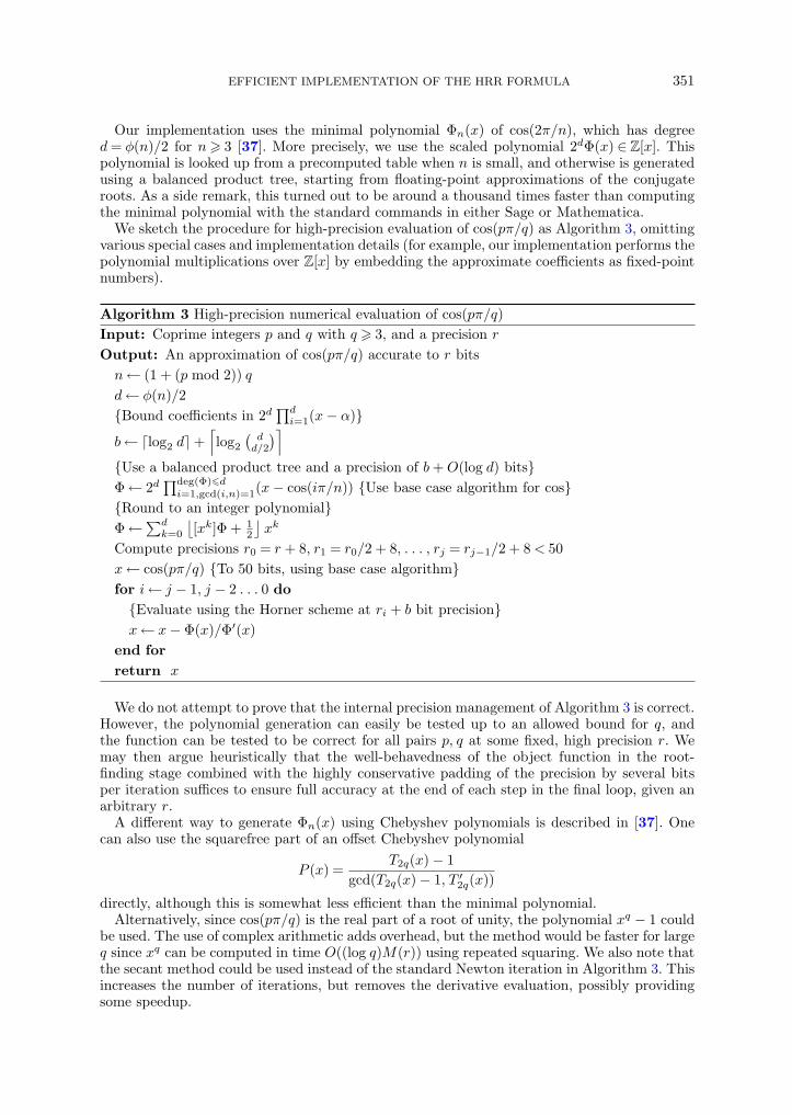
Our implementation uses the minimal polynomial Φn(x) of cos(2π/n), which has degreed= φ(n)/2 for n> 3 [37]. More precisely, we use the scaled polynomial 2dΦ(x) ∈ Z[x]. Thispolynomial is looked up from a precomputed table when n is small, and otherwise is generatedusing a balanced product tree, starting from floating-point approximations of the conjugateroots. As a side remark, this turned out to be around a thousand times faster than computingthe minimal polynomial with the standard commands in either Sage or Mathematica.

We sketch the procedure for high-precision evaluation of cos(pπ/q) as Algorithm 3, omittingvarious special cases and implementation details (for example, our implementation performs thepolynomial multiplications over Z[x] by embedding the approximate coefficients as fixed-pointnumbers).

Algorithm 3 High-precision numerical evaluation of cos(pπ/q)Input: Coprime integers p and q with q > 3, and a precision r

Output: An approximation of cos(pπ/q) accurate to r bitsn← (1 + (p mod 2)) qd← φ(n)/2Bound coefficients in 2d

∏di=1(x− α)

b← dlog2 de+⌈log2

(dd/2

)⌉Use a balanced product tree and a precision of b+O(log d) bitsΦ← 2d

∏deg(Φ)6di=1,gcd(i,n)=1(x− cos(iπ/n)) Use base case algorithm for cos

Round to an integer polynomialΦ←

∑dk=0

⌊[xk]Φ + 1

2

⌋xk

Compute precisions r0 = r + 8, r1 = r0/2 + 8, . . . , rj = rj−1/2 + 8< 50x← cos(pπ/q) To 50 bits, using base case algorithmfor i← j − 1, j − 2 . . . 0 doEvaluate using the Horner scheme at ri + b bit precisionx← x− Φ(x)/Φ′(x)

end forreturn x

We do not attempt to prove that the internal precision management of Algorithm 3 is correct.However, the polynomial generation can easily be tested up to an allowed bound for q, andthe function can be tested to be correct for all pairs p, q at some fixed, high precision r. Wemay then argue heuristically that the well-behavedness of the object function in the root-finding stage combined with the highly conservative padding of the precision by several bitsper iteration suffices to ensure full accuracy at the end of each step in the final loop, given anarbitrary r.

A different way to generate Φn(x) using Chebyshev polynomials is described in [37]. Onecan also use the squarefree part of an offset Chebyshev polynomial

P (x) =T2q(x)− 1

gcd(T2q(x)− 1, T ′2q(x))

directly, although this is somewhat less efficient than the minimal polynomial.Alternatively, since cos(pπ/q) is the real part of a root of unity, the polynomial xq − 1 could

be used. The use of complex arithmetic adds overhead, but the method would be faster for largeq since xq can be computed in time O((log q)M(r)) using repeated squaring. We also note thatthe secant method could be used instead of the standard Newton iteration in Algorithm 3. Thisincreases the number of iterations, but removes the derivative evaluation, possibly providingsome speedup.

352 F. JOHANSSON

In our implementation, Algorithm 3 was found to be faster than the MPFR trigonometricfunctions for q < 250 roughly when the precision exceeds 400 + 4q2 bits. This estimate includesthe cost of generating the minimal polynomial on the fly.

3.7. The main algorithm

Algorithm 4 outlines the main routine in FLINT with only minor simplifications. To avoidpossible corner cases in the convergence of the HRR sum, and to avoid unnecessary overhead,values with n < 128 (exactly corresponding to p(n)< 232) are looked up from a table. We onlyuse k, n, N in Theorem 4 in order to make the precision decrease uniformly, allowing amortizedsummation to be implemented in a simple way.

Algorithm 4 Main routine implementing the HRR formulaInput: n> 128Output: p(n)

Determine N and initial precision r1 using Theorem 4C← π

6

√24n− 1 At r1 + 3 bits

u← exp(C)s1← s2← 0for 1 6 k 6N do

Write term k as (3.2) by calling Algorithm 2if Ak(n) 6= 0 then

Determine term precision rk for |tk| using Theorem 4Use Algorithm 3 if qi < 250 and rk > 400 + 4q2t← (−1)s

√a/b

∏cos(piπ/qi)

t← t× U(C/k) Compute U from u1/k if k < 35Amortized summation: r(s2) denotes precision of the variable s2s2← s2 + tif 2rk < r(s2) thens1← s1 + s2 Exactly or with precision exceeding r1r(s2)← rk Change precisions2← 0

end ifend if

end forreturn bs1 + s2 + 1

2c

Since our implementation presently relies on some numerical heuristics (and in any case,considering the intricacy of the algorithm), care has been taken to test it extensively. All n6 106

have been checked explicitly, and a large number of isolated n 106 have been comparedagainst known congruences and values computed with Sage and Mathematica.

As a strong robustness check, we observe experimentally that the numerical error in the finalsum decreases with larger n. For example, the error is consistently smaller than 10−3 for n > 106

and smaller than 10−4 for n > 109. This phenomenon reflects the fact that (1.8) overshoots theactual magnitude of the terms with large k, combined with the fact that rounding errors averageout pseudorandomly rather than approaching worst-case bounds.

4. Benchmarks

Table 1 and Figure 1 compare performance of Mathematica 7, Sage 4.7 and FLINT on a laptopwith a Pentium T4400 2.2 GHz CPU and 3 GB of RAM, running 64 bit Linux. To the author’s

EFFICIENT IMPLEMENTATION OF THE HRR FORMULA 353

104 105 106 107 108 109 1010 1011 1012 1013 1014 1015 1016

Tim

e (s

)

n

105

104

103

102

101

100

10–1

10–2

10–3

10–4

Figure 1. CPU time t in seconds for computing p(n): FLINT (blue squares), Mathematica 7 (greencircles), Sage 4.7 (red triangles). The dotted line shows t = 10−6n1/2, indicating the slope of an

idealized algorithm satisfying the trivial lower complexity bound Ω(n1/2) (the offset 10−6 isarbitrary).

knowledge, Mathematica and Sage contain the fastest previously available partition functionimplementations by far.

The FLINT code was run with MPIR version 2.4.0 and MPFR version 3.0.1. Since Sage 4.7uses an older version of MPIR and Mathematica is based on an older version of GMP, differencesin performance of the underlying arithmetic slightly skew the comparison, but probably notby more than a factor of two.

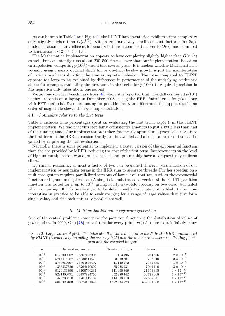
The limited memory of the aforementioned laptop restricted the range of feasible n toapproximately 1016. Using a system with an AMD Opteron 6174 processor and 256 GB RAMallowed calculating p(1017), p(1018) and p(1019) as well. The last computation took just lessthan 100 hours and used more than 150 GB of memory, producing a result with over 11 billionbits. Some large values of p(n) are listed in Table 2.

Table 1. Timings for computing p(n) in Mathematica 7, Sage 4.7 and FLINT up to n = 1016 on thesame system, as well as FLINT timings for n = 1017–1019 (*) done on different (slightly faster)hardware. Calculations running less than one second were repeated, allowing benefits from datacaching. The rightmost column shows the amount of time in the FLINT implementation spent

computing the first term.

n Mathematica 7 Sage 4.7 FLINT Initial (%)

104 69 ms 1 ms 0.20 ms105 250 ms 5.4 ms 0.80 ms106 590 ms 41 ms 2.74 ms107 2.4 s 0.38 s 0.010 s108 11 s 3.8 s 0.041 s109 67 s 42 s 0.21 s 43

1010 340 s 0.88 s 531011 2 116 s 5.1 s 481012 10 660 s 20 s 491013 88 s 481014 448 s 471015 2 024 s 391016 6 941 s 451017 27 196* s 331018 87 223* s 381019 350 172* s 39

354 F. JOHANSSON

As can be seen in Table 1 and Figure 1, the FLINT implementation exhibits a time complexityonly slightly higher than O(n1/2), with a comparatively small constant factor. The Sageimplementation is fairly efficient for small n but has a complexity closer to O(n), and is limitedto arguments n < 232 ≈ 4× 109.

The Mathematica implementation appears to have complexity slightly higher than O(n1/2)as well, but consistently runs about 200–500 times slower than our implementation. Based onextrapolation, computing p(1019) would take several years. It is unclear whether Mathematica isactually using a nearly-optimal algorithm or whether the slow growth is just the manifestationof various overheads dwarfing the true asymptotic behavior. The ratio compared to FLINTappears too large to be explained by differences in performance of the underlying arithmeticalone; for example, evaluating the first term in the series for p(1010) to required precision inMathematica only takes about one second.

We get one external benchmark from [4], where it is reported that Crandall computed p(109)in three seconds on a laptop in December 2008, ‘using the HRR ‘finite’ series for p(n) alongwith FFT methods’. Even accounting for possible hardware differences, this appears to be anorder of magnitude slower than our implementation.

4.1. Optimality relative to the first term

Table 1 includes time percentages spent on evaluating the first term, exp(C), in the FLINTimplementation. We find that this step fairly consistently amounts to just a little less than halfof the running time. Our implementation is therefore nearly optimal in a practical sense, sincethe first term in the HRR expansion hardly can be avoided and at most a factor of two can begained by improving the tail evaluation.

Naturally, there is some potential to implement a faster version of the exponential functionthan the one provided by MPFR, reducing the cost of the first term. Improvements on the levelof bignum multiplication would, on the other hand, presumably have a comparatively uniformeffect.

By similar reasoning, at most a factor of two can be gained through parallelization of ourimplementation by assigning terms in the HRR sum to separate threads. Further speedup on amulticore system requires parallelized versions of lower level routines, such as the exponentialfunction or bignum multiplication. (A simplistic multithreaded version of the FLINT partitionfunction was tested for n up to 1018, giving nearly a twofold speedup on two cores, but failedwhen computing 1019 for reasons yet to be determined.) Fortunately, it is likely to be moreinteresting in practice to be able to evaluate p(n) for a range of large values than just for asingle value, and this task naturally parallelizes well.

5. Multi-evaluation and congruence generation

One of the central problems concerning the partition function is the distribution of values ofp(n) mod m. In 2000, Ono [28] proved that for every prime m> 5, there exist infinitely many

Table 2. Large values of p(n). The table also lists the number of terms N in the HRR formula usedby FLINT (theoretically bounding the error by 0.25) and the difference between the floating-point

sum and the rounded integer.

n Decimal expansion Number of digits Terms Error

1012 6129000962 . . . 6867626906 1 113 996 264 526 2 × 10−7

1013 5714414687 . . . 4630811575 3 522 791 787 010 3 × 10−8

1014 2750960597 . . . 5564896497 11 140 072 2 350 465 −1 × 10−8

1015 1365537729 . . . 3764670692 35 228 031 7 043 140 −3 × 10−9

1016 9129131390 . . . 3100706231 111 400 846 21 166 305 −9 × 10−10

1017 8291300791 . . . 3197824756 352 280 442 63 775 038 5 × 10−10

1018 1478700310 . . . 1701612189 1 114 008 610 192 605 341 4 × 10−10

1019 5646928403 . . . 3674631046 3 522 804 578 582 909 398 4 × 10−11

EFFICIENT IMPLEMENTATION OF THE HRR FORMULA 355

congruences of the type

p(Ak +B)≡ 0 mod m (5.1)

where A, B are fixed and k ranges over all nonnegative integers. Ono’s proof is nonconstructive,but Weaver [38] subsequently gave an algorithm for finding congruences of this type whenm ∈ 13, 17, 19, 23, 29, 31, and used the algorithm to compute 76 065 explicit congruences.

Weaver’s congruences are specified by a tuple (m, `, ε) where ` is a prime and ε ∈ −1, 0, 1,where we unify the notation by writing (m, `, 0) in place of Weaver’s (m, `). Such a tuplecorresponds to a family of congruences of the form (5.1) with coefficients

A=m`4−|ε| (5.2)

B =m`3−|ε|α+ 1

24+m`3−|ε|δ, (5.3)

where α is the unique solution of m`3−|ε|α≡−1 mod 24 with 1 6 α < 24, and where 0 6 δ < `is any solution of

24δ 6≡ −α mod ` if ε= 0(24δ + α | `) = ε if ε=±1.

(5.4)

The free choice of δ gives `− 1 distinct congruences for a given tuple (m, `, ε) if ε= 0, and(`− 1)/2 congruences if ε=±1.

Weaver’s test for congruence, described by [38, Theorems 7 and 8], essentially amounts to asingle evaluation of p(n) at a special point n. Namely, for given m, `, we compute the smallestsolutions of δm ≡ 24−1 mod m, rm ≡−m mod 24, and check whether p(mrm(`2 − 1)/24 + δm)is congruent mod m to one of three values corresponding to the parameter ε ∈ −1, 0, 1. Wegive a compact statement of this procedure as Algorithm 5. To find new congruences, we simplyperform a brute force search over a set of candidate primes `, calling Algorithm 5 repeatedly.

Algorithm 5 Weaver’s congruence testInput: A pair of prime numbers 13 6m6 31 and `> 5, m 6= `

Output: (m, `, ε) defining a congruence, and Not-a-congruence otherwise

δm← 24−1 mod m Reduced to 0 6 δm <mrm← (−m) mod 24 Reduced to 0 6m< 24v← m− 3

2x← p(δm) We have x 6≡ 0 mod m

y← p

(m

(rm(`2 − 1)

24

)+ δm

)f ← (3 | `) ((−1)vrm | `) Jacobi symbolst← y + fx`v−1

if t≡ ω mod m where ω ∈ −1, 0, 1 then

return (m, `, ω (3(−1)v | `))else

return Not-a-congruence

end if

356 F. JOHANSSON

5.1. Comparison of algorithms for vector computation

In addition to the HRR formula, the author has added code to FLINT for computing the vectorof values p(0), p(1), . . . , p(n) over Z and Z/mZ. The code is straightforward, simply calling thedefault FLINT routines for power series inversion over the respective coefficient rings, whichin both cases invokes Newton iteration and FFT multiplication via Kronecker segmentation.

A timing comparison between the various methods for vector computation is shown inTable 3. The power series method is clearly the best choice for computing all values up ton modulo a fixed prime, having a complexity of O(n1+o(1)). For computing the full integervalues, the power series and HRR methods both have complexity O(n3/2+o(1)), with the powerseries method expectedly winning.

Ignoring logarithmic factors, we can expect the HRR formula to be better than the powerseries for multi-evaluation of p(n) up to some bound n when n/c values are needed. The factorc≈ 10 in the FLINT implementation is a remarkable improvement over c≈ 1000 attainablewith previous implementations of the partition function. For evaluation mod m, the HRRformula is competitive when O(n1/2) values are needed; in this case, the constant is highlysensitive to m.

For the sparse subset of O(n1/2) terms searched with Weaver’s algorithm, the HRR formulahas the same complexity as the modular power series method, but as seen in Table 3 runs morethan an order of magnitude faster. On top of this, it has the advantage of parallelizing trivially,being resumable from any point, and requiring very little memory (the power series evaluationmod m= 13 up to n= 109 required over 40 GB memory, compared to a few megabytes withthe HRR formula). Euler’s method is, of course, also resumable from an arbitrary point, butthis requires computing and storing all previous values.

We mention that the authors of [7] use a parallel version of the recursive Euler method.This is not as efficient as power series inversion, but allows the computation to be split acrossmultiple processors more easily.

5.2. Results

Weaver gives 167 tuples, or 76 065 congruences, containing all ` up to approximately 1000–3000(depending on m). This table was generated by computing all values of p(n) with n < 7.5× 106

using the recursive version of Euler’s pentagonal theorem. Computing Weaver’s table fromscratch with FLINT, evaluating only the necessary n, takes just a few seconds. We are alsoable to numerically verify instances of all entries in Weaver’s table for small k.

As a more substantial exercise, we extend Weaver’s table by determining all ` up to 106 foreach prime m. Statistics are listed in Table 4. The computation was performed by assigningsubsets of the search space to separate processes, running on between 40 and 48 active coresfor a period of four days, evaluating p(n) at 6(π(106)− 3) = 470 970 distinct n ranging up to2× 1013.

Table 3. Comparison of time needed to compute multiple values of p(n) up to the given bound,using power series inversion and the HRR formula. The rightmost column gives the time when only

computing the subset of terms that are searched with Weaver’s algorithm in the m = 13 case.

n Series (Z/13Z) Series (Z) HRR (all) HRR (sparse)

104 0.01 s 0.1 s 1.4 s 0.001 s105 0.13 s 4.1 s 41 s 0.008 s106 1.4 s 183 s 1430 s 0.08 s107 14 s 0.7 s108 173 s 8 s109 2507 s 85 s

EFFICIENT IMPLEMENTATION OF THE HRR FORMULA 357

We find a total of 70 359 tuples, corresponding to slightly more than 2.2 × 1010

new congruences. To pick an arbitrary, concrete example, one ‘small’ new congruence is(13, 3797,−1) with δ = 2588, giving

p(711647853449k + 485138482133)≡ 0 mod 13

which we easily evaluate for all k 6 100, providing a sanity check on the identity as well as thepartition function implementation. As a larger example, (29, 999 959, 0) with δ = 999 958 gives

p(28995244292486005245947069k + 28995221336976431135321047)≡ 0 mod 29

which, despite our efforts, presently is out of reach for direct evaluation.Complete tables of (`, ε) for each m are available at:

http://www.risc.jku.at/people/fjohanss/partitions/http://sage.math.washington.edu/home/fredrik/partitions/.

6. Discussion

Two obvious improvements to our implementation would be to develop a rigorous, and perhapsfaster, version of Algorithm 3 for computing cos(pπ/q) to high precision, and to develop fastmultithreaded implementations of transcendental functions to allow computing p(n) for muchlarger n. Curiously, a particularly simple AGM-type iteration is known for exp(π) (see [3]), andit is tempting to speculate whether a similar algorithm can be constructed for exp(π

√24n− 1),

allowing faster evaluation of the first term.Some performance could also be gained with faster low-precision transcendental functions

(up to a few thousand bits) and by using a better bound than (1.8) for the truncation error.The algorithms described in this paper can be adapted to evaluation of other HRR-type

series, such as the number of partitions into distinct parts

Q(n) =π2√

224

∞∑k=1

A2k−1(n)(1− 2k)2 0F1

(2,

(n+ 124 )π2

12(1− 2k)2

). (6.1)

Using asymptotically fast methods for numerical evaluation of hypergeometric functions, itshould be possible to retain quasi-optimality.

Finally, it remains an open problem whether there is a fast way to compute the isolatedvalue p(n) using purely algebraic methods. We mention the interesting recent work by Bruinierand Ono [6], which perhaps could lead to such an algorithm.

Acknowledgements. The author thanks Silviu Radu for suggesting the application ofextending Weaver’s table of congruences, and for explaining Weaver’s algorithm in detail.The author also thanks the anonymous referee for various suggestions, and Jonathan Bober

Table 4. The number of tuples of the given type with ` < 106, the total number of congruencesdefined by these tuples, the total CPU time, and the approximate bound up to which p(n) was

evaluated.

m (m, `, 0) (m, `,+1) (m, `, −1) Congruences CPU (h) Max n

13 6 189 6 000 6 132 5 857 728 831 448 5.9 × 1012

17 4 611 4 611 4 615 4 443 031 844 391 4.9 × 1012

19 4 114 4 153 4 152 3 966 125 921 370 3.9 × 1012

23 3 354 3 342 3 461 3 241 703 585 125 9.5 × 1011

29 2 680 2 777 2 734 2 629 279 740 1 155 2.2 × 1013

31 2 428 2 484 2 522 2 336 738 093 972 2.1 × 1013

All 23 376 23 367 23 616 22 474 608 014 3 461

358 F. JOHANSSON

for pointing out that Erdos’ theorem about quadratic nonresidues gives a rigorous complexitybound without assuming the Extended Riemann Hypothesis.

Finally, William Hart gave valuable feedback on various issues, and generously providedaccess to the computer hardware used for the large-scale computations reported in this paper.The hardware was funded by Hart’s EPSRC Grant EP/G004870/1 (Algorithms in AlgebraicNumber Theory) and hosted at the University of Warwick.

References

1. N. Ankeny, ‘The least quadratic non residue’, Ann. of Math. (2) 55 (1952) no. 1, 65–72.2. T. Apostol, Modular functions and Dirichlet series in number theory, 2nd edn (Springer, New York,

1997).3. J. Borwein and D. Bailey, Mathematics by experiment: plausible reasoning in the 21st century (A K

Peters, Wellesley, MA, 2003) 137.4. J. Borwein and P. Borwein, Experimental and computational mathematics: selected writings (Perfectly

Scientific Press, Portland, OR, 2010) 250.5. R. Brent and P. Zimmermann, Modern computer arithmetic (Cambridge University Press, New York,

2011).6. J. Bruinier and K. Ono, ‘Algebraic formulas for the coefficients of half-integral weight harmonic weak

Maass forms’, Preprint, 2011, arXiv.org/abs/1104.1182.7. N. Calkin, J. Davis, K. James, E. Perez and C. Swannack, ‘Computing the integer partition function’,

Math. Comp. 76 (2007) no. 259, 1619–1638.8. M. Cipolla, ‘Un metodo per la risoluzione della congruenza di secondo grado’, Napoli Rend. 9 (1903)

153–163.9. R. Crandall and C. Pomerance, Prime numbers: a computational perspective (Springer, New York,

2005) 99–103.10. P. Erdos, ‘Remarks on number theory. I’, Mat. Lapok 12 (1961) 10–17.11. A. Fousse, G. Hanrot, V. Lefevre, P. Pelissier and P. Zimmermann, ‘MPFR: A multiple-precision

binary floating-point library with correct rounding’, ACM Trans. Math. Software 33, no. 2, 2007,http://www.mpfr.org/.

12. The GMP development team, ‘Computing billions of π digits using GMP’, http://gmplib.org/pi-with-gmp.html.

13. The GMP development team, ‘GMP: the GNU multiple precision arithmetic library’, http://gmplib.org/.14. P. Hagis Jr, ‘A root of unity occurring in partition theory’, Proc. Amer. Math. Soc 26 (1970) no. 4,

579–582.15. G. H. Hardy and S. Ramanujan, ‘Asymptotic formulae in combinatory analysis’, Proc. Lond. Math. Soc.

17 (1918) 75–115.16. W. Hart, ‘Fast library for number theory: an introduction’, Mathematical software – ICMS 2010, Lecture

Notes in Computer Science 6327, 88–91, http://www.flintlib.org.17. W. Hart, ‘A one line factoring algorithm’, J. Aust. Math. Soc. 92 (2012) 61–69.18. N. Higham, Accuracy and stability of numerical algorithms, 2nd edn (SIAM, Philadelphia, 2002).19. Intel corporation, Pentium processor family developer’s manual. Volume 3: architecture and programming

manual, 1995, http://www.intel.com/design/pentium/MANUALS/24143004.pdf.20. D. Knuth, ‘Notes on generalized Dedekind sums’, Acta Arith. 33 (1977) 297–325.21. D. Knuth, Fascicle 3: generating all combinations and partitions, The Art of Computer Programming,

vol. 4 (Addison-Wesley, 2005).22. D. Lehmer, ‘On the series for the partition function’, Trans. Amer. Math. Soc. 43 (1938) no. 2, 271–295.23. D. Lehmer, ‘On a conjecture of Ramanujan’, J. Lond. Math. Soc. 11 (1936) 114–118.24. D. Lehmer, ‘On the Hardy–Ramanujan series for the partition function’, J. Lond. Math. Soc. 3 (1937)

171–176.25. The MPIR development team, ‘MPIR: multiple precision integers and rationals’, http://www.mpir.org.26. A. Odlyzko, ‘Asymptotic enumeration methods’, Handbook of combinatorics 2 (eds R. Graham, M.

Grotschel and L. Lovasz; Elsevier, The Netherlands, 1995) 1063–1229,http://www.dtc.umn.edu/∼odlyzko/doc/asymptotic.enum.pdf.

27. OEIS Foundation Inc, ‘The on-line encyclopedia of integer sequences’, 2011, http://oeis.org/A000041.28. K. Ono, ‘The distribution of the partition function modulo m’, Ann. of Math. (2) 151 (2000) 293–307.29. The Pari/GP development team, ‘Pari/GP, Bordeaux’, 2011, http://pari.math.u-bordeaux.fr/.30. P. Pollack, ‘The average least quadratic nonresidue modulo m and other variations on a theme of Erdos’,

J. Number Theory 132 (2012) no. 6, 1185–1202.31. H. Rademacher, ‘On the partition function p(n)’, Proc. Lond. Math. Soc. 43 (1938) 241–254.32. H. Rademacher and A. Whiteman, ‘Theorems on Dedekind sums’, Amer. J. Math. 63 (1941) no. 2,

377–407.33. D. Shanks, ‘Five number-theoretic algorithms’, Proceedings of the Second Manitoba Conference on

Numerical Mathematics, 1972, 51–70.

EFFICIENT IMPLEMENTATION OF THE HRR FORMULA 359

34. W. Stein and The Sage development team, ‘Sage: open source mathematics software’, http://www.sagemath.org.

35. Sun Microsystems Inc, ‘FDLIBM version 5.3’, http://www.netlib.org/fdlibm/readme.36. A. Tonelli, ‘Bemerkung uber die Auflosung quadratischer Congruenzen’, Gottinger Nachrichten (1891)

344–346.37. W. Watkins and J. Zeitlin, ‘The minimal polynomial of cos(2π/n)’, Amer. Math. Monthly 100 (1993)

no. 5, 471–474.38. R. Weaver, ‘New congruences for the partition function’, J. Ramanujan 5 (2001) 53–63.39. A. Whiteman, ‘A sum connected with the series for the partition function’, Pacific J. Math. 6 (1956) no. 1,

159–176.40. Wolfram Research Inc., ’Some notes on internal implementation’, Mathematica documentation center,

2011, http://reference.wolfram.com/mathematica/note/SomeNotesOnInternalImplementation.html.41. P. Zimmermann, The bit-burst algorithm, Slides presented at computing by the numbers: algorithms,

precision, and complexity, Berlin, 2006, http://www.loria.fr/∼zimmerma/talks/arctan.pdf.

Fredrik JohanssonResearch Institute for Symbolic

ComputationJohannes Kepler UniversityAltenberger Strasse 69, 4040 LinzAustria

fredrik.johansson@risc.jku.at