Chapter 3

Building physical 3D models

Fig. 3.1: A CNC routed model of the Sonoma Valley, California

Tangible Landscape works with many types of physical 3D models. Whenused as a continuous shape display the physical model should be built of amalleable material such as sand, clay, or wax so that users can easily deformthe surface. When used for object recognition the physical model can be builtof a rigid material such as a wood product, plastic, or resin. When both modesof interaction are combined the physical model should use malleable materialsfor the base and rigid materials for the objects. These models can be builtby hand or digitally fabricated using 3D printing or computer numericallycontrolled (CNC) manufacturing.

The final model should be opaque, have a light color, and have a mattefinish so that the projected image is crisp and vivid. Transparent materialslike acrylic cannot be 3D scanned with a Kinect. Some 3D printing and cast-ing materials like resin may appear opaque, but have translucent properties– this will diffuse the projection. If we desire a very crisp and vivid image on

33

34 3 Building physical 3D models

a rigid model made of wood products or resins we recommend painting themodel white.

In this chapter we discuss different types of physical models and explainhow to fabricate them.

3.1 Handmade models

Fig. 3.2: Sculpting a polymeric sand model

Rigid physical models can be handmade by hand-cutting contours andmalleable physical models can be handmade by sculpting sand or clay.

Contour models can be precise if they are finely cut, but they are inaccu-rate as they depict abstract, stepped landscapes that are discrete rather thancontinuous. They are also very legible – one can easily count the contours andread the height – but again they represent abstracted landscapes. While onecan easily read the contours and then calculate slope, it is hard to intuitivelyvisualize the slope. Furthermore this abstract, discontinuous representationmay obfuscate the relationship between form and process. Furthermore theyare time consuming and complicated to construct especially for complex to-pographies. Hand cutting contour models can be dangerous as the knife mayslip or jump.

Contour models can be made out of stacked boards of paperboard, card-board, foam, or a soft wood like balsa or basswood. The thickness of the

3.2 Digitally fabricated models 35

sheets should correspond to the vertical interval between contours at the de-sired map scale. To build a contour model by hand start by plotting a contourmap at the desired map scale. Then spray the plotted paper map with a spraymount adhesive, and stick the plotted map onto a board. As an alternative toplotting and mounting, we can instead project the contour map. Cut out thelowest contour level with a precision knife such an x-acto. Glue this contourlevel onto the base or the level below. Repeat this process until all of thecontour levels have been cut out and stacked together.

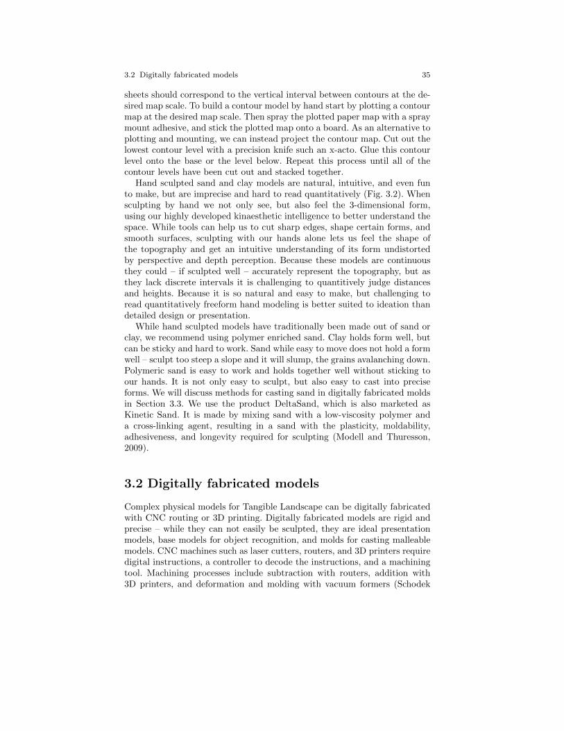
Hand sculpted sand and clay models are natural, intuitive, and even funto make, but are imprecise and hard to read quantitatively (Fig. 3.2). Whensculpting by hand we not only see, but also feel the 3-dimensional form,using our highly developed kinaesthetic intelligence to better understand thespace. While tools can help us to cut sharp edges, shape certain forms, andsmooth surfaces, sculpting with our hands alone lets us feel the shape ofthe topography and get an intuitive understanding of its form undistortedby perspective and depth perception. Because these models are continuousthey could – if sculpted well – accurately represent the topography, but asthey lack discrete intervals it is challenging to quantitively judge distancesand heights. Because it is so natural and easy to make, but challenging toread quantitatively freeform hand modeling is better suited to ideation thandetailed design or presentation.

While hand sculpted models have traditionally been made out of sand orclay, we recommend using polymer enriched sand. Clay holds form well, butcan be sticky and hard to work. Sand while easy to move does not hold a formwell – sculpt too steep a slope and it will slump, the grains avalanching down.Polymeric sand is easy to work and holds together well without sticking toour hands. It is not only easy to sculpt, but also easy to cast into preciseforms. We will discuss methods for casting sand in digitally fabricated moldsin Section 3.3. We use the product DeltaSand, which is also marketed asKinetic Sand. It is made by mixing sand with a low-viscosity polymer anda cross-linking agent, resulting in a sand with the plasticity, moldability,adhesiveness, and longevity required for sculpting (Modell and Thuresson,2009).

3.2 Digitally fabricated models

Complex physical models for Tangible Landscape can be digitally fabricatedwith CNC routing or 3D printing. Digitally fabricated models are rigid andprecise – while they can not easily be sculpted, they are ideal presentationmodels, base models for object recognition, and molds for casting malleablemodels. CNC machines such as laser cutters, routers, and 3D printers requiredigital instructions, a controller to decode the instructions, and a machiningtool. Machining processes include subtraction with routers, addition with3D printers, and deformation and molding with vacuum formers (Schodek

36 3 Building physical 3D models

et al., 2004, chap. 13). In this section we will explain how to prepare GISdata for digital fabrication and discuss various methods of digital fabrication.Section 3.4 describes workflows for creating models using these methods.

3.2.1 Digital models

Terrain and other continuous, 3D geographic data can be digitally repre-sented as 3D points, 2.5D rasters, 3D rasters, contours, meshes, or surfaces.In GRASS GIS our workflows for landscape modeling and analysis are rasterbased. 3D printers and CNC routers, however, require vector data, typicallymeshes. After acquiring elevation data we import them into GRASS GIS andif necessary we interpolate a raster digital elevation model (DEM). This rasterwill later be used as the reference data for Tangible Landscape. Next, we ex-port the raster as a point cloud and import it into a 3D modeling program tocompute a surface, mesh, or solid from the point cloud. Finally, we generatea toolpath from the surface or mesh for the 3D printer or CNC router.

The first step in modeling a landscape is to acquire data. Entire landscapescan be precisely 3D scanned as point clouds with airborne lidar. As pulses oflight are emitted from the aircraft they hit and reflect back from vegetation,structures, and topography. When a pulse of light hits a tree part of thelight is reflected and recorded as the first return, while the rest penetratesthe outer canopy. The residual pulse, recorded as a series of returns, reflectsoff of leaves, branches, shrubs, and the ground. Lidar data can be used tocompute very precise, high resolution models. By filtering lidar returns andclasses we can extract points for the bare earth topography and interpolate araster DEM or we can extract points with all of the structures and vegetationand interpolate a raster digital surface model (DSM). Lidar point clouds orready to use raster DEMs are available for many locations and are well suitedfor building topographic models (see Appendix A.2 for links to lidar data andDEM repositories).

DEMs – raster maps of bare earth topography – and DSMs – raster mapsof topography with structures and vegetation – are commonly used in GISto represent and analyze terrain as they can easily be mathematically trans-formed. For example topographic parameters such as slope, aspect, and curva-ture can be computed from the partial derivatives of a function approximatinga DEM or DSM (see chapter 4). Data structures such as image pyramidsand quadtrees are an efficient and effective way of storing, analyzing, andvisualizing large datasets.

Lidar, especially when filtered by classes or returns, can produce scat-tered, spatially heterogeneous data points that are challenging to accuratelyinterpolate as terrain surfaces. Furthermore, other sources of elevation datasuch as digitized contours and surveying data can be clustered and have ahighly spatially heterogeneous distribution. The regularized spline with ten-sion (RST) interpolation function, implemented as the v.surf.rst module inGRASS GIS, can be used to accurately model terrain surfaces from clustered

3.2 Digitally fabricated models 37

and heterogeneous data such as lidar with some experimentation and tuning(See 4.1.2).

Contour data are challenging to interpolate because the data are spatiallyheterogenous – they are often very dense along the contour lines with largeunsampled areas in regions with flat topography. If we acquire digital contourdata we can either linearly interpolate between contours with r.surf.contouror thin the points along contours using v.generalize, convert them to a pointrepresentation and then interpolate them using a function like RST with themodule v.surf.rst (The GRASS GIS Community, 2015).

Terrain can also be modeled in 3D vector representations such as polygonmeshes or mathematically defined surfaces. In a mesh a vector network ofpolygons such as triangles or quadrilaterals forms a shape. Terrain meshesare typically triangulated irregular networks (TINs) that connect the datapoints from which they are computed. Triangulation was used to manuallyinterpolate contours from surveyed spot elevations before the advent of com-puters. Now TINs are typically computed using the Delaunay triangulationalgorithm which maximizes the smallest angle of every triangle in order tominimize the occurrence of very thin triangles. Since TINs connect the datapoints the input data is preserved. When meshes are low resolution, i.e. com-puted from small datasets, they reveal their polygonal structure with angledplanes where there should be curved surfaces. When meshes are high res-olution, i.e. computed from large datasets, they can be very detailed andrepresent highly complex forms. Even a high resolution mesh, however, isinaccurate when used to represent curved slopes as planar faces. Meshes arevery useful for modeling structures and engineered topography with discon-tinuous slopes.

Non-uniform rational B-splines (NURBs) are parametric approximationcurves and surfaces defined by a series of polynomials. The curves are ba-sis splines defined by a knot vector, weighted control points, and the curve’sorder or degree (Piegl and Tiller, 1995). A NURBS surface is the tensor prod-uct of two NURBS curves (Martisek and Prochazkova, 2010). Since NURBSsurfaces are mathematically defined they can precisely describe a continuousgeometry.

Processed lidar data and rasters can be exported as point clouds fromGIS and then imported into a 3D modeling program for meshing or sur-face generation. Toolpaths for CNC routing can be generated for a mesh orNURBS surface once it has been scaled. 3D printing, however, requires closed,solid volumes so the terrain surface should be offset or extruded to give it athickness. Most 3D printers read the stereolithography (.stl) format, a meshrepresentation of a solid.

38 3 Building physical 3D models

We typically use Rhinoceros for 3D modeling1 with the RhinoTerrain plu-gin for terrain modeling2 and the RhinoCAM plugin for CNC routing.3 Thisproprietary 3D modeling program is useful for its interoperability – it canwrite and read a wide range of formats and can model NURBS, polygonmeshes, solids, and point clouds. The RhinoTerrain plugin has modules forimporting and exporting geographic data and efficiently computing largeterrain meshes. While many CAM programs require polygon meshes, theRhinoCAM plugin enables us to generate and simulate CNC toolpaths inRhinoceros using NURBS, polygon meshes, or solids. The Rhino3DPRINTplugin can be used to prepare models for 3D printing.4 Alternatives includea proprietary 3D modeling and animation program,5 or MeshLab, an opensource mesh processing program.6

3.2.2 Laser cutting

Laser cutting can be used to efficiently build precise contour models of mod-erate complexity (Fig. 3.3). Laser cutters are CNC machines that use a lasermoving along a gantry in the x and y axes to make 2D cuts. To laser cuta contour model we separate each contour step onto different layers of a 2Dvector drawing in a computer aided design (CAD) format (like .dwg, .dxf, or.ai). We cut each contour step out of a sheet of our material of choice andglue them together. We can also laser etch elevation values, patterns, and linework like road outlines and building footprints onto each layer. While it iseasy to precisely cut complex topographies it is still challenging to constructthem as we have to lay and glue each piece by hand.

The materials determine the cost. As this is a subtractive method a lotof material is wasted. Contour models cut from thick, low-cost materials likecardboard are relatively inexpensive, but have large contour steps and thuslow resolution. Models cut from thin, low-cost materials like chipboard allowfor small contour steps at moderate cost, but tend to warp with time espe-cially if too much glue has been applied. When aesthetics and archivabilityare important museum board or acrylic can be cut to create presentation-quality laser cut contour models. Paper-based media such as chipboard ormuseum board are not suitable for casting polymeric sand as the polymerwill stick and soak into them.

1 Rhinoceros: http://www.rhino3d.com/2 RhinoTerrain: http://www.rhinoterrain.com/3 RhinoCAM: http://mecsoft.com/rhinocam-software/4 Rhino3DPRINT: http://mecsoft.com/rhino3dprint/5 Maya: http://www.autodesk.com/products/maya/overview6 MeshLab: http://meshlab.sourceforge.net/

3.2 Digitally fabricated models 39

Fig. 3.3: A laser cut chipboard contour model with basswood buildings fab-ricated by David Koontz and Faustine Pastor

40 3 Building physical 3D models

3.2.3 CNC routing

CNC routing or milling is a subtractive fabrication process that can be used toprecisely manufacture contour models and surface models of great complexity(Fig. 3.4). This type of digital fabrication is a precise, accurate, inexpensive,and scalable way to build terrain models. 3-axis CNC routers and millingmachines move a spindle with a machining bit along the x, y, and z axes ina programmed path to carve a shape out of a block of material (Fig. 3.5).Because 3-axis routers can only carve vertically they produce 2.5D surfacemodels on a solid base, rather than full 3D volumetric models. It is possible,however, to manufacture fully 3D volumes with 3-axis routers; after each cutone can reorient the model and then route the sides or bottom of the model(Schodek et al., 2004, chap. 14).

Fig. 3.4: A CNC routed terrain model of the Jockey’s Ridge dune complexon the Outer Banks of North Carolina

To CNC route a terrain model we first prepare a solid block of our material.We can use materials such as medium to high density foam, wax, and woodproducts. We typically use medium density fiberboard (MDF) or baltic birch,engineered wood products with high strength, good dimensional stability, anda fine, uniform grain with minimal voids. To prepare MDF we cut the sheetinto tiles that match the desired extent of our scale model, spread wood glue

3.2 Digitally fabricated models 41

Fig. 3.5: A 3-axis CNC router carving a terrain model

evenly over each tile and stack the tiles together, and firmly clamp the stackof tiles together until the glue sets (Fig. 3.6).

(a) Pour glue onto a layerof MDF

(b) Spread glue evenlyover a layer of MDF

(c) Stack layers of MDF

(d) Clamp the stack ofMDF

(e) Add a weight on topof the stack of MDF

(f) Wait for the glue todry

Fig. 3.6: Preparing MDF for CNC routing

42 3 Building physical 3D models

In a CAD program we prepare a digital model of the geometry we wish tocarve. Then we generate a toolpath for this digital model in a computer aidedmanufacturing (CAM) program. To make a contour model we use closed, 3Dcontour curves as our data and then carve with a contour cut. Contour cut-ting can also be used to carve buildings. To carve a surface model from a meshor NURBs surface we use parallel cuts. For a surface model we typically startwith a horizontal rough cut with a 0.5 inch diameter, carbide bit to removethe bulk of the excess material (Table 3.1). Then we use a parallel finish cutwith a 0.25 inch diameter, carbide, ball-nose bit to carve the the terrain as acontinuous surface (Table 3.2). If we need a more refined presentation-qualitymodel we then make two more parallel finish cuts in alternative cutting direc-tions with a 0.125 inch diameter, carbide, ball-nose bit to smooth the surfaceand capture more detail. Finally a contour cut along the border can be usedto neatly trim and remove the model from the base material. The toolpath iswritten as a sequence of instructions in a CNC programming language oftenas a .nc file in G-Code. The CNC machine’s controller reads this code anddrives the tool along the toolpath carving our model. We have a streamlinedworkflow using Rhinoceros with the RhinoCAM plugin for both 3D model-ing and the generation, simulation, and visualization of toolpaths. We do ourCAD and CAM in the same environment – Rhinoceros – so that we can easilyedit our models and work with both meshes and NURBS.

Once the model has been routed we may want to finish it by sanding, prim-ing, and painting the model. Sanding the model, a prerequisite for primingand painting, with a fine grit sandpaper produces a smoother surface. Afterrouting and sanding we clean the model with an air hose. Applying severalcoats of magnetic primer to our model weakly magnetizes it so that magne-tized markers stick to the slopes (Fig. 3.7). A magnetized model is useful forTangible Landscape applications relying on object recognition rather thansculpting. Finally we may want to spray paint our model white to enhancethe brightness of projected imagery.

Table 3.1: CNC settings: horizontal rough cut with MDF

Bit ∅ Speed Plunge Approach Engage Cut Retract Departure Step down Stepover

0.5 inch 16000 65 135 205 275 800 800 0.32 inch 48%

0.25 inch 16000 50 75 125 175 800 800 0.25 inch 40%

3.2.4 3D printing

With 3D printing, a type of solid freeform fabrication, we can make a com-plex, 3D volume in a single run. While the models can be precise, accurate,and highly complex, they are also expensive and small as 3D printers have

3.2 Digitally fabricated models 43

Fig. 3.7: A marker with a magnetic base sticking to CNC-routed terrain modelprimed with magnetic paint

(a) (b)

Fig. 3.8: Modes of interaction using markers: (a) rasterizing an area and (b)drawing a polygon.

Table 3.2: CNC settings: parallel finish cut with MDF

Bit ∅ Speed Plunge Approach Engage Cut Retract Departure Stepover

0.5 inch 16000 65 160 230 325 800 800 20%

0.25 inch 16000 50 100 150 225 800 800 20%

44 3 Building physical 3D models

restrictively small build areas and the materials are relatively expensive. 3Dprinting is an ideal process for fabricating small, complex models such asbuildings or small, high quality presentation models for use with TangibleLandscape (Fig. 3.9a).

While CNC milling and routing are subtractive processes, 3D printing isan additive process in which a model is built up layer by layer. A digital, 3D,solid model is divided into a stack of horizontal layers or slices and a toolpathis computed for each slice. The physical model is then built slice by slice bydepositing or hardening material along the toolpath. By dividing the modelinto cross sections, each as thin as the technology allows, a complex volumecan be formed. There are a variety of different 3D printing processes includingstereolithography, selective laser sintering, fused deposition modeling, and3D ink-jet printing each with tradeoffs in build speed, quality, strength, cost,resolution, color, and material (Schodek et al., 2004, chap. 14).

3.3 Molding and casting

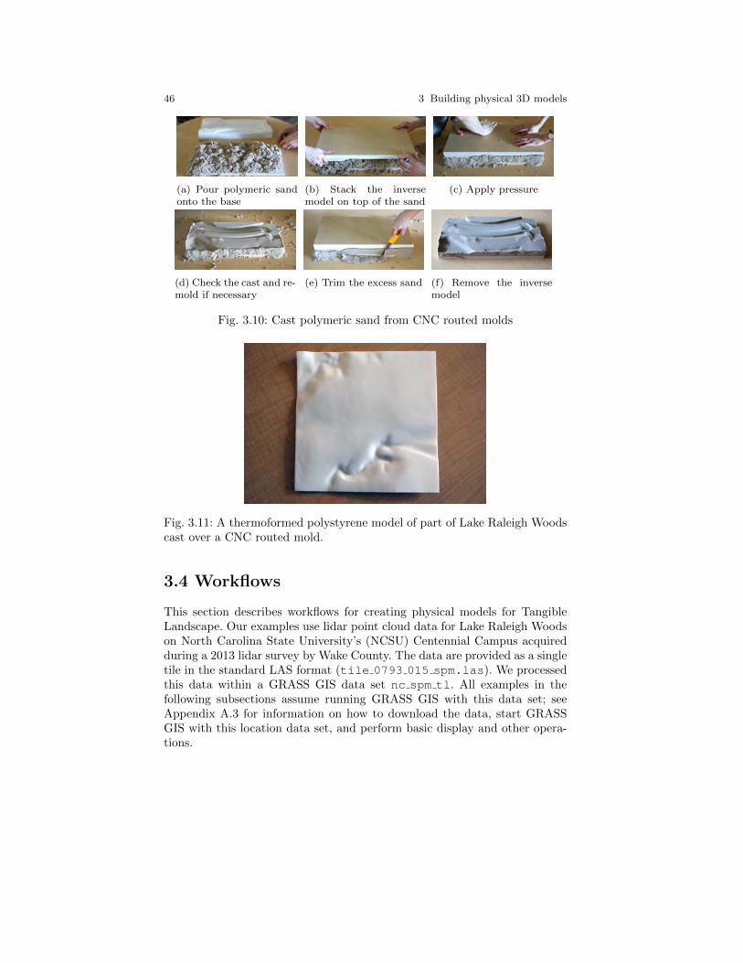
To sculpt with Tangible Landscape we need a malleable model made of asoft, deformable medium. A model made of polymer enriched sand is easy tosculpt, holds its form well, and can be cast into precise forms. CNC routedand 3D printed models can be used as molds for casting polymeric sandinto malleable models. The mold should be the inverse of the surface thatwill be cast. Cast models can precisely represent complex forms that are toochallenging to model by hand and can easily be recast.

To cast a terrain model either CNC route the inverse of the terrain(Fig. 3.10) or 3D print the terrain as a volume extruded with enough thick-ness to survive the casting process (Fig. 3.9). We press the mold into thepolymeric sand to cast the form. We have to check the cast and repeat theprocess if necessary – sand may need to be added or removed in places toget a good cast. Clamps can be used to get strong, even pressure on a CNCrouted mold when casting.

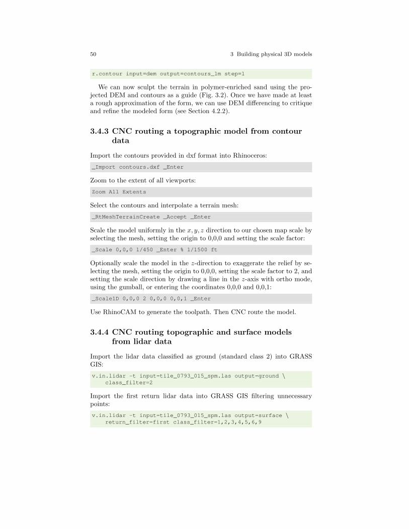
Thermoforming or vacuuming forming can be used to quickly make lightweightcopies or imprints of a CNC routed terrain model in a thermoplastic. Sincethey are lightweight thermoformed models are very portable and are idealfor casting polymeric sand while traveling. To thermoform a terrain modelwe heat a thermoplastic sheet in a vacuum former until it becomes soft. Usethe vacuum to pull the hot plastic over a mold deforming the plastic into thedesired shape. Once the plastic cools into the cast shape we release the vac-uum. We may need to drill small holes through our mold to make a completevacuum (Schodek et al., 2004, chap. 14).

3.3 Molding and casting 45

(a) 3D prints of the terrain and canopy

(b) Casting sand with 3D prints

(c) The canopy cast in sand

(d) The terrain cast in sand

Fig. 3.9: Casting polymeric sand from 3D printed molds

46 3 Building physical 3D models

(a) Pour polymeric sandonto the base

(b) Stack the inversemodel on top of the sand

(c) Apply pressure

(d) Check the cast and re-mold if necessary

(e) Trim the excess sand (f) Remove the inversemodel

Fig. 3.10: Cast polymeric sand from CNC routed molds

Fig. 3.11: A thermoformed polystyrene model of part of Lake Raleigh Woodscast over a CNC routed mold.

3.4 Workflows

This section describes workflows for creating physical models for TangibleLandscape. Our examples use lidar point cloud data for Lake Raleigh Woodson North Carolina State University’s (NCSU) Centennial Campus acquiredduring a 2013 lidar survey by Wake County. The data are provided as a singletile in the standard LAS format (tile 0793 015 spm.las). We processedthis data within a GRASS GIS data set nc spm tl. All examples in thefollowing subsections assume running GRASS GIS with this data set; seeAppendix A.3 for information on how to download the data, start GRASSGIS with this location data set, and perform basic display and other opera-tions.

3.4 Workflows 47

(a) (b)

Fig. 3.12: 3D renderings of terrain models derived from lidar tile 0793 015using (a) GRASS GIS and (b) Rhinoceros with the RhinoTerrain plugin (seeSection 3.4.4)

3.4.1 Selecting a 3D model scale

The scale of the physical 3D model depends on the extent of the data, thedesired model size, and the desired scale. The scale may also depend on thematerial of the model, the scanning technology, and the resolution of thedata. Here we assume that we know the spatial extent of our data and wantour model to be approximately half a meter long on each side. If we do notalready know the extent of our data we can determine the values once thedata has been imported into GRASS GIS for example using v.info or r.info.

We can perform this computation in the Python interactive console. First,we enter the spatial extent of the data and approximate the size of the model(in meters):

n = 224028.45s = 223266.45e = 639319.28w = 638557.28desired_model_x = 0.50

Then we compute the scale using the equation:

s =dmdr

(3.1)

where s is the scale of the model, dm is the distance measured on the model,and dr is the real-world distance. For convenience we can also compute thescale number using the equation:

sn =1

s(3.2)

where sn is the scale number of the model and s is the scale of the model.We then type the following in the Python console:

48 3 Building physical 3D models

scale = desired_model_x / (n - s)scale_number = 1. / scale

The scale is now 1 : 1524 and the scale number is 1524. Since we want thescale to be a round number and do not want to add or remove data we needto modify the scale and reverse the computation in the previous step so thatwe can compute the new size of the model at the selected scale. We select ascale of 1 : 1500 (a round value close to the previously computed scale). InPython we then write:

scale_number = 1500scale = 1. / scale_numbermodel_x = (n - s) * scale

The resulting model size is 50.8 cm.So far we have only used the spatial extent along the north-south direction.

We skipped the east-west direction because the extent of both the data andthe model were squares. In a region with an elongated rectangular shape wemight need to determine a suitable scale for each of the horizontal directionsand then decide on a compromise.

Next we determine the vertical size of the model and its vertical exagger-ation. First, we enter the minimum and maximum elevation in the dataset(called top and bottom in GRASS GIS) and we also include the desiredheight of the model (in meters). In our example we set the desired height ofthe model to 0.04 m:

t = 109.33b = 76.54desired_model_h = 0.04

Then we compute the model height without vertical exaggeration and theexaggeration based on the desired model height using the equation:

e =heh

(3.3)

where e is the exaggeration, he is the exaggerated height (in our case thedesired height of the model) and h is the height of the model according tothe scale in case the model would not be exaggerated.

Since we already know the scale of the model from the previous com-putations we can now compute the exaggeration and model height withoutvertical exaggeration:

model_h = scale * (t - b)exaggeration = desired_model_h / model_h

With the given the inputs the exaggeration is now approximately 1.8. Sincewe want a round number we set the vertical exaggeration to 2 and computethe actual height of the model using Eq. 3.3:

3.4 Workflows 49

exaggeration = 2actual_model_h = exaggeration * model_h

With the exaggeration set to 2 the model height (or more precisely the maxi-mum height difference of the top surface of the model) will be approximately4.4 cm. The base of the model will increase the actual model height. Depend-ing on how it is constructed the base may or may not be an integral partof the model. If we set the exaggeration to 1.5 the model height differencewould be approximately 3.3 cm, which might be too shallow. At a differentscale, however, an exaggeration of 1.5 might be the right choice.

We have used the same scale in both the x and y horizontal directions(1 : 1500). However, in the vertical direction (z) we exaggerated the scale bya factor of 2. As a result the vertical scale (1 : 750) is different than horizontalscale (1 : 1500). Depending on the audience it may be advantageous to noteeither the horizontal and vertical scales or the scale and exaggeration. Whenthe scale and exaggeration are known the vertical scale can be computedusing the equation:

sv = se (3.4)

where sv is the vertical scale, s is the horizontal scale and e is the exaggera-tion. Once we have computed the size of our model we can build the modelusing any of the methods described in the following sections.

3.4.2 Sculpting a malleable model from data

A simple way to create a malleable 3D model is to sculpt the landscapein polymer-enriched sand using projected contours derived from DEM asa guide. In this workflow we used a point cloud of elevation data in theLAS format (tile 0793 015 spm.las) and worked in the GRASS GISlocation nc spm tl. To sculpt a malleable model from lidar data performthe following steps:

Import the lidar points classified as ground (standard class 2) into GRASSGIS using the module v.in.lidar :

v.in.lidar -t input=tile_0793_015_spm.las output=ground \class_filter=2

Set the region to the spatial extent of the imported tile and resolution to1 m. Then interpolate the DEM from the processed lidar data:

g.region vect=ground res=1v.surf.rst -t input=ground elevation=dem tension=100 npmin=250 \

dmin=2

Check the results, adjust the parameters, and rerun with the overwrite flagif necessary. Then compute the 1 m interval contours from the DEM:

50 3 Building physical 3D models

r.contour input=dem output=contours_1m step=1

We can now sculpt the terrain in polymer-enriched sand using the pro-jected DEM and contours as a guide (Fig. 3.2). Once we have made at leasta rough approximation of the form, we can use DEM differencing to critiqueand refine the modeled form (see Section 4.2.2).

3.4.3 CNC routing a topographic model from contourdata

Import the contours provided in dxf format into Rhinoceros:

_Import contours.dxf _Enter

Zoom to the extent of all viewports:

Zoom All Extents

Select the contours and interpolate a terrain mesh:

_RtMeshTerrainCreate _Accept _Enter

Scale the model uniformly in the x, y, z direction to our chosen map scale byselecting the mesh, setting the origin to 0,0,0 and setting the scale factor:

_Scale 0,0,0 1/450 _Enter % 1/1500 ft

Optionally scale the model in the z-direction to exaggerate the relief by se-lecting the mesh, setting the origin to 0,0,0, setting the scale factor to 2, andsetting the scale direction by drawing a line in the z-axis with ortho mode,using the gumball, or entering the coordinates 0,0,0 and 0,0,1:

_Scale1D 0,0,0 2 0,0,0 0,0,1 _Enter

Use RhinoCAM to generate the toolpath. Then CNC route the model.

3.4.4 CNC routing topographic and surface modelsfrom lidar data

Import the lidar data classified as ground (standard class 2) into GRASSGIS:

v.in.lidar -t input=tile_0793_015_spm.las output=ground \class_filter=2

Import the first return lidar data into GRASS GIS filtering unnecessarypoints:

v.in.lidar -t input=tile_0793_015_spm.las output=surface \return_filter=first class_filter=1,2,3,4,5,6,9

3.4 Workflows 51

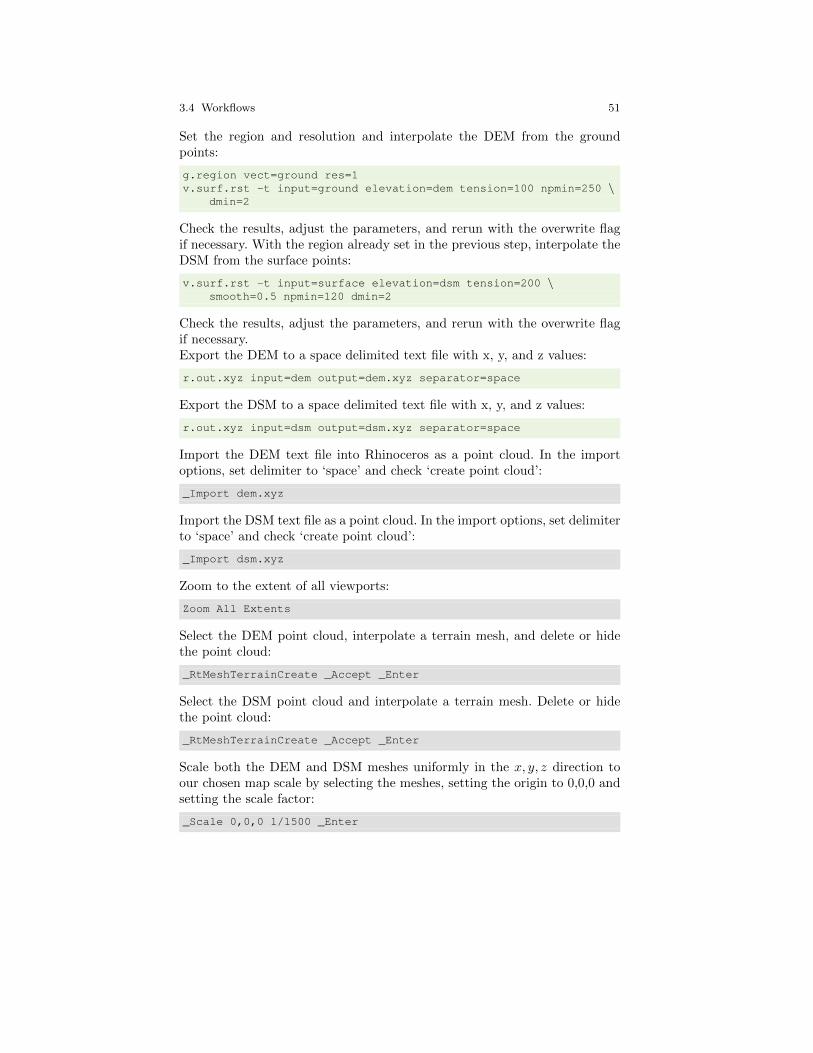
Set the region and resolution and interpolate the DEM from the groundpoints:

g.region vect=ground res=1v.surf.rst -t input=ground elevation=dem tension=100 npmin=250 \

dmin=2

Check the results, adjust the parameters, and rerun with the overwrite flagif necessary. With the region already set in the previous step, interpolate theDSM from the surface points:

v.surf.rst -t input=surface elevation=dsm tension=200 \smooth=0.5 npmin=120 dmin=2

Check the results, adjust the parameters, and rerun with the overwrite flagif necessary.Export the DEM to a space delimited text file with x, y, and z values:

r.out.xyz input=dem output=dem.xyz separator=space

Export the DSM to a space delimited text file with x, y, and z values:

r.out.xyz input=dsm output=dsm.xyz separator=space

Import the DEM text file into Rhinoceros as a point cloud. In the importoptions, set delimiter to ‘space’ and check ‘create point cloud’:

_Import dem.xyz

Import the DSM text file as a point cloud. In the import options, set delimiterto ‘space’ and check ‘create point cloud’:

_Import dsm.xyz

Zoom to the extent of all viewports:

Zoom All Extents

Select the DEM point cloud, interpolate a terrain mesh, and delete or hidethe point cloud:

_RtMeshTerrainCreate _Accept _Enter

Select the DSM point cloud and interpolate a terrain mesh. Delete or hidethe point cloud:

_RtMeshTerrainCreate _Accept _Enter

Scale both the DEM and DSM meshes uniformly in the x, y, z direction toour chosen map scale by selecting the meshes, setting the origin to 0,0,0 andsetting the scale factor:

_Scale 0,0,0 1/1500 _Enter

52 3 Building physical 3D models

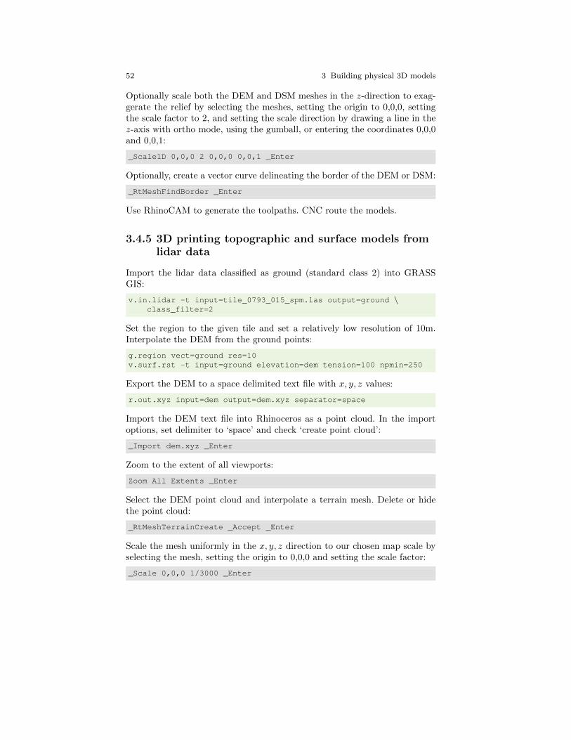
Optionally scale both the DEM and DSM meshes in the z-direction to exag-gerate the relief by selecting the meshes, setting the origin to 0,0,0, settingthe scale factor to 2, and setting the scale direction by drawing a line in thez-axis with ortho mode, using the gumball, or entering the coordinates 0,0,0and 0,0,1:

_Scale1D 0,0,0 2 0,0,0 0,0,1 _Enter

Optionally, create a vector curve delineating the border of the DEM or DSM:

_RtMeshFindBorder _Enter

Use RhinoCAM to generate the toolpaths. CNC route the models.

3.4.5 3D printing topographic and surface models fromlidar data

Import the lidar data classified as ground (standard class 2) into GRASSGIS:

v.in.lidar -t input=tile_0793_015_spm.las output=ground \class_filter=2

Set the region to the given tile and set a relatively low resolution of 10m.Interpolate the DEM from the ground points:

g.region vect=ground res=10v.surf.rst -t input=ground elevation=dem tension=100 npmin=250

Export the DEM to a space delimited text file with x, y, z values:

r.out.xyz input=dem output=dem.xyz separator=space

Import the DEM text file into Rhinoceros as a point cloud. In the importoptions, set delimiter to ‘space’ and check ‘create point cloud’:

_Import dem.xyz _Enter

Zoom to the extent of all viewports:

Zoom All Extents _Enter

Select the DEM point cloud and interpolate a terrain mesh. Delete or hidethe point cloud:

_RtMeshTerrainCreate _Accept _Enter

Scale the mesh uniformly in the x, y, z direction to our chosen map scale byselecting the mesh, setting the origin to 0,0,0 and setting the scale factor:

_Scale 0,0,0 1/3000 _Enter

3.4 Workflows 53

Optionally scale the mesh in the z-direction to exaggerate the relief by se-lecting the mesh, setting the origin to 0,0,0, setting the scale factor to 2, andsetting the scale direction by drawing a line in the z-axis with ortho mode,using the gumball, or entering the coordinates 0,0,0 and 0,0,1:

_Scale1D 0,0,0 2 0,0,0 0,0,1 _Enter

Create a vector curve delineating the border of the DEM:

_RtMeshFindBorder _Enter

Prepare the mesh for 3D printing. Select the border curve as the boundaryand the DEM mesh as the mesh. Set offset to relative or absolute. Set a baseheight:

_RtMesh3dPrintPrepare

Export the selected mesh as a stereolithography file (.stl) and send it to the3D printer:

_-SaveAs

3.4.6 Casting a malleable topographic model with aCNC routed mold derived from lidar data

Import the lidar data classified as ground (standard class 2) into GRASSGIS:

v.in.lidar -t input=tile_0793_015_spm.las output=ground \class_filter=2

Set the region and resolution, then interpolate the DEM from the groundpoints:

g.region vect=ground res=1v.surf.rst -t input=ground elevation=dem tension=100 npmin=250 \

dmin=2

Check the results, adjust the parameters, and rerun with the overwrite flagif necessary.Export the DEM to a space delimited text file with x, y, z values:

r.out.xyz input=dem output=dem.xyz separator=space

Import the DEM text file into Rhinoceros as a point cloud. In the importoptions, set delimiter to ‘space’ and check ‘create point cloud’:

_Import dem.xyz _Enter

Zoom to the extent of all viewports:

Zoom All Extents _Enter

54 3 Building physical 3D models

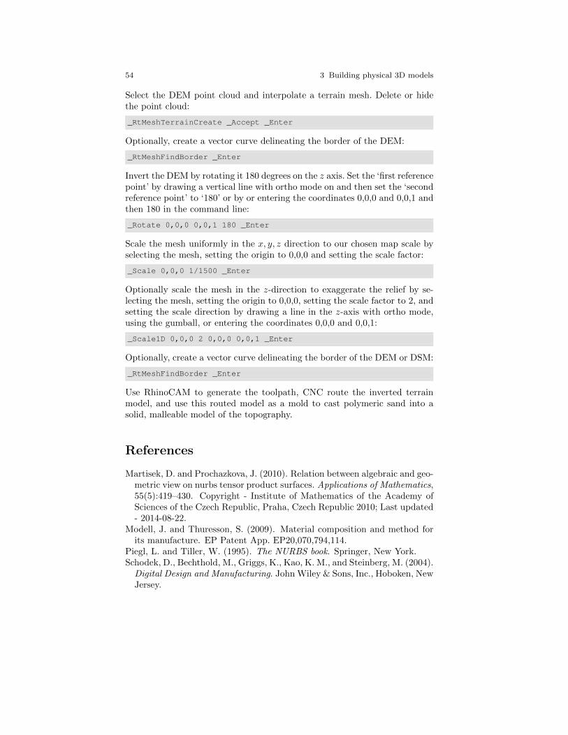
Select the DEM point cloud and interpolate a terrain mesh. Delete or hidethe point cloud:

_RtMeshTerrainCreate _Accept _Enter

Optionally, create a vector curve delineating the border of the DEM:

_RtMeshFindBorder _Enter

Invert the DEM by rotating it 180 degrees on the z axis. Set the ‘first referencepoint’ by drawing a vertical line with ortho mode on and then set the ‘secondreference point’ to ‘180’ or by or entering the coordinates 0,0,0 and 0,0,1 andthen 180 in the command line:

_Rotate 0,0,0 0,0,1 180 _Enter

Scale the mesh uniformly in the x, y, z direction to our chosen map scale byselecting the mesh, setting the origin to 0,0,0 and setting the scale factor:

_Scale 0,0,0 1/1500 _Enter

Optionally scale the mesh in the z-direction to exaggerate the relief by se-lecting the mesh, setting the origin to 0,0,0, setting the scale factor to 2, andsetting the scale direction by drawing a line in the z-axis with ortho mode,using the gumball, or entering the coordinates 0,0,0 and 0,0,1:

_Scale1D 0,0,0 2 0,0,0 0,0,1 _Enter

Optionally, create a vector curve delineating the border of the DEM or DSM:

_RtMeshFindBorder _Enter

Use RhinoCAM to generate the toolpath, CNC route the inverted terrainmodel, and use this routed model as a mold to cast polymeric sand into asolid, malleable model of the topography.

References

Martisek, D. and Prochazkova, J. (2010). Relation between algebraic and geo-metric view on nurbs tensor product surfaces. Applications of Mathematics,55(5):419–430. Copyright - Institute of Mathematics of the Academy ofSciences of the Czech Republic, Praha, Czech Republic 2010; Last updated- 2014-08-22.

Modell, J. and Thuresson, S. (2009). Material composition and method forits manufacture. EP Patent App. EP20,070,794,114.

Piegl, L. and Tiller, W. (1995). The NURBS book. Springer, New York.Schodek, D., Bechthold, M., Griggs, K., Kao, K. M., and Steinberg, M. (2004).

Digital Design and Manufacturing. John Wiley & Sons, Inc., Hoboken, NewJersey.

References 55

The GRASS GIS Community. Contour lines to DEM [online].(2015) [Accessed 2015-05-28]. http://grasswiki.osgeo.org/wiki/Contour_lines_to_DEM.