Chapter 19 More Complex ANOVA Designs - WordPress.com · Chapter 19 More Complex ANOVA Designs This...
46
Chapter 19 More Complex ANOVA Designs This chapter examines three designs that incorporate more factors and in- troduce some new elements of experimental design. They are three-way ANOVA, one-way nested ANOVA, and analysis of covariance (ANCOVA). These are common designs whose elements can be combined to generate even more elaborate ones. A useful guide to complex ANOVA designs is Winer et al. (1991), who provide a description and statistical model for each design. Once a particular design is identified, the statistical model can be used to program the analysis in SAS or other software. 19.1 Three-way ANOVA We will first discuss three-way ANOVA, an analysis which examines how three different factors influence the means of the different groups. The three factors may be any combination of fixed or random effects and are typically referred to a Factors A, B, and C. In this design, there are one or more repli- cate observations for each combination of the three factors. The statistical analysis for three-way ANOVA designs may include F tests for the main ef- fects of the factors as well as the interactions among them. For example, if the design has replication and all three factors are fixed, there are F tests for the main effects (Factor A, B, C), each pairwise interaction (A × B, A × C, B × C), and a three-way interaction (A × B × C). The additional complexity of this design with its many interactions can make interpretation 609
Transcript of Chapter 19 More Complex ANOVA Designs - WordPress.com · Chapter 19 More Complex ANOVA Designs This...

Chapter 19
More Complex ANOVADesigns
This chapter examines three designs that incorporate more factors and in-troduce some new elements of experimental design. They are three-wayANOVA, one-way nested ANOVA, and analysis of covariance (ANCOVA).These are common designs whose elements can be combined to generate evenmore elaborate ones. A useful guide to complex ANOVA designs is Winer etal. (1991), who provide a description and statistical model for each design.Once a particular design is identified, the statistical model can be used toprogram the analysis in SAS or other software.
19.1 Three-way ANOVA
We will first discuss three-way ANOVA, an analysis which examines howthree different factors influence the means of the different groups. The threefactors may be any combination of fixed or random effects and are typicallyreferred to a Factors A, B, and C. In this design, there are one or more repli-cate observations for each combination of the three factors. The statisticalanalysis for three-way ANOVA designs may include F tests for the main ef-fects of the factors as well as the interactions among them. For example, ifthe design has replication and all three factors are fixed, there are F testsfor the main effects (Factor A, B, C), each pairwise interaction (A × B, A× C, B × C), and a three-way interaction (A × B × C). The additionalcomplexity of this design with its many interactions can make interpretation
609

610 CHAPTER 19. MORE COMPLEX ANOVA DESIGNS
of the results quite challenging.As an example of three-way ANOVA, we will analyze data from an ex-
periment by Maestre & Reynolds (2007). This study examined how overallnutrient and water availability, and nutrient heterogeneity, affected grasslandbiomass production (Table 19.1). Nutrient heterogeneity was manipulated byplacing the nitrogen at a particular location within the container vs. an evendistribution. See Chapter 14 for further description of this experiment. Wewill use the notation Yijkl to reference the observations in three-way ANOVAdesigns. The i subscript refers to the group or treatment within Factor A (inthis case nitrogen heterogeneity), j the treatment within Factor B (nitrogenlevels), k the treatment within Factor C (water levels), while l refers to theobservation within the treatment. For example, Y1134 refers to the fourth ob-servation in the no nutrient heterogeneity, 40 mg N, 375 ml water treatment,which is 7.901.

19.1.THREE-W
AY
ANOVA
611Table 19.1: Example 1 - Effect of nitrogen heterogeneity, nitrogen availability, and water availability on thetotal biomass of grassland plants grown in microcosms (Maestre & Reynolds 2007). The table illustrateshow the subscripts for Yijkl vary across treatments for a portion of the data set (see Chapter 21 for the fullversion).
N het. (Y/N) N (mg) Water (ml/week) Yijkl = Biomass i j k lN 40 125 4.372 1 1 1 1N 40 125 4.482 1 1 1 2N 40 125 4.221 1 1 1 3N 40 125 3.977 1 1 1 4N 40 250 7.400 1 1 2 1N 40 250 8.027 1 1 2 2N 40 250 7.883 1 1 2 3N 40 250 7.769 1 1 2 4N 40 375 7.226 1 1 3 1N 40 375 8.126 1 1 3 2N 40 375 6.840 1 1 3 3N 40 375 7.901 1 1 3 4
etc.
Y 120 250 10.731 2 3 2 1Y 120 250 12.640 2 3 2 2Y 120 250 10.350 2 3 2 3Y 120 250 11.550 2 3 2 4Y 120 375 14.697 2 3 3 1Y 120 375 17.826 2 3 3 2Y 120 375 14.711 2 3 3 3Y 120 375 13.614 2 3 3 4

612 CHAPTER 19. MORE COMPLEX ANOVA DESIGNS
19.1.1 Three-way fixed effects model
Suppose that we want to model the observations in a study like Example1, where there are Factors A, B, and C. Assume the design is factorial withevery possible combination of the three factors, with n > 1 observations ofeach one. This design is often called three-way ANOVA with replication. Acommon model for the observations Yijkl in such designs (Winer et al. 1991)is
Yijkl = µ+αi +βj + +γk + (αβ)ij + (βγ)jk + (αγ)ik + (αβγ)ijk + εijkl. (19.1)
Here µ is the grand mean of the observations, while αi is the deviation fromµ caused by the ith level or treatment of Factor A, βj the deviation causedby the jth level of Factor B, and γk is the deviation caused by the kth level ofFactor C. These terms are the main effects in the model. The terms (αβ)ij,(βγ)jk, and (αγ)ik are pairwise or first-order interactions among Factors Aand B, B and C, and A and C. These interactions are also symbolized as A× B, B × C, and A × C. They are similar to the interaction term in two-wayANOVA, but with three factors in the design there are more possibilities forinteraction among them. The term (αβγ)ijk models a second-order interac-tion (symbolized as A × B × C) among all three factors. It can be thoughtof as an interaction of interactions, i.e., the interaction between Factors Aand B could change across levels of C. The εijkl term represents the usualrandom departures from the mean value predicted by the main effects andinteractions due to natural variability.
The objective in three-way ANOVA is to test whether Factor A, B, andC have an effect on the group means, and whether there are interactionsamong these factors. For Factor A this amounts to testing H0 : all αi = 0,and similarly H0 : all βj = 0 for Factor B and H0 : all γk = 0 for FactorC. For the A × B interaction, we would test H0 : (αβ)ij = 0, and similarlyH0 : (αγ)ik = 0 for the A × C and H0 : (βγ)jk = 0 for the B × C interactions.For the second-order interaction A × B × C, we are interested in testing H0 :all (αβγ)ijk = 0. The F tests for these hypotheses can be constructed usingvarious sums of squares and mean squares, similar to two-way ANOVA, andare also examples of likelihood ratio tests. We will not consider this processin detail but instead proceed directly to the analysis and interpretation ofthe Example 1 data set.

19.1. THREE-WAY ANOVA 613
19.1.2 Three-way ANOVA for Example 1 - SAS demo
The first step in the program (see below) is to read in the observationsusing a data step, with the first variable (nitrohet) denoting the nitrogenheterogeneity treatment, while nitrogen and water represent the nitrogen andwater levels. The variable biomass is then log-transformed before analysis,yielding the dependent variable y = log10(biomass}. Three separate plotsthen requested using proc gplot (SAS Institute Inc. 2014a), one for everypairwise combination of nitrohet, nitrogen, and water. These plots will allowus to examine the main effects and all first order (pairwise) interactionsamong the treatments. The choice as to whether a particular treatment isplotted on the x-axis or appears as separate groups (lines) on the graph isarbitrary. Like two-way ANOVA, if the lines are not parallel in a plot thissuggests there is an interaction between the factors.
The second set of plots is intended to illustrate the second-order interac-tion among the three factors. Each plot illustrates the interaction betweennitrogen and water at one level of nitrogen heterogeneity. If there is a second-order interaction, then the plots will appear different from one another.
The next section of the program conducts the three-way ANOVA usingproc glm (SAS Institute Inc. 2014b). The class statement tells SAS thatnitrohet, nitrogen, and water are used to classify the observations into the 18different treatment groups. The model statement tells SAS the form of theANOVA model. Recall that the model for fixed effects three-way ANOVA(Eq. 19.1). The statement nitrohet|nitrogen|water is SAS shorthand forthis model, and will automatically generate all the possible main effects andinteractions of the three factors.
The lsmeans statement causes proc glm to calculate quantities called leastsquares means for each level of nitrohet, nitrogen, and water. When the dataare balanced these are equivalent to the means for each treatment group, butleast squares means have some advantages for unbalanced data and otherstatistical models. The option adjust=tukey requests multiple comparisonsamong treatments using the Tukey method. This is useful for comparing thedifferent levels of the main effects. However, tests for the main effects as wellas multiple comparisons should be treated with caution in the presence ofstrong interaction (see Chapter 14 for discussion of this issue).
We now examine the results of the tests generated by SAS, examiningthe interactions first (see SAS output below). We are primarily interestedin the results for Type III sums of squares. We see that the second-order

614 CHAPTER 19. MORE COMPLEX ANOVA DESIGNS
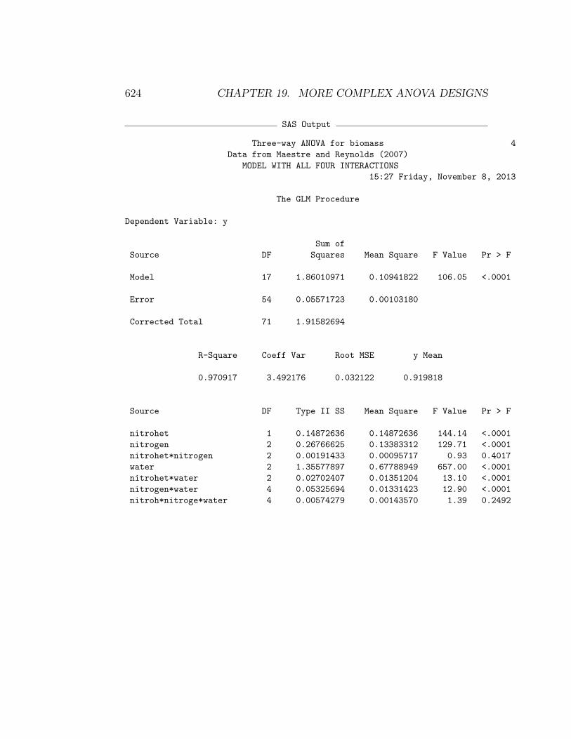
nitrogen heterogeneity × nitrogen × water interaction was nonsignificant(F4,54 = 1.39, P = 0.2492). The two graphs that illustrate this interaction ap-pear similar, further indicating this interaction is weak or absent (Fig. 19.1,19.2). Turning to the first order interactions, we see that the nitrogen hetero-geneity × nitrogen interaction was nonsignificant (F2,54 = 0.93, P = 0.4017).In agreement with this result, the corresponding graph for this interaction(Fig. 19.3) suggests these two treatments are additive. The nitrogen ×water interaction (F4,54 = 12.90, P < 0.0001) was highly significant. Ex-amining Fig. 19.4, we see that the source of this interaction was a reducedeffect of watering at lower nitrogen levels. The nitrogen heterogeneity ×water interaction was also highly significant (F2,54 = 13.10, P < 0.0001).This interaction was apparently generated by a stronger effect of nitrogenheterogeneity at the lowest water level (Fig. 19.5). Overall, the significantinteractions suggest that effects of these factors on biomass are not additive(Maestre & Reynolds 2007).
The SAS analysis also found highly significant main effects of nitrogenheterogeneity (F1,54 = 144.14, P < 0.0001), nitrogen (F2,27 = 129.71, P <0.0001) and water (F2,27 = 657.00, P < 0.0001) on biomass. We can judgethe strength of these effects through the interaction plots as well as the sumof squares values. Watering appears to have the largest effect on biomass,followed by nitrogen and nitrogen heterogeneity. The heterogeneity result isparticularly intriguing, because more biomass was generated when this nu-trient was heterogeneously distributed in space. Maestre & Reynolds (2007)suggest this occurred because nutrient patches encourage root proliferation,leading to increased nutrient uptake and overall growth. Even though therewere significant interactions in this analysis, the main effects were larger andexplained most of the variation in these data.
19.1. THREE-WAY ANOVA 615
SAS program
* Maestre_biomass_3way.sas;
options pageno=1 linesize=80;
goptions reset=all;
title "Three-way ANOVA for biomass";
title2 "Data from Maestre and Reynolds (2007)";
data maestre;
input nitrohet $ nitrogen water biomass;
* Apply transformations here;
y = log10(biomass);
datalines;
N 40 125 4.372
N 40 125 4.482
N 40 125 4.221
N 40 125 3.977
N 40 250 7.400
N 40 250 8.027
N 40 250 7.883
N 40 250 7.769
etc.
Y 120 375 14.697
Y 120 375 17.826
Y 120 375 14.711
Y 120 375 13.614
;
run;
* Print data set;
proc print data=maestre;
run;
proc gplot data=maestre;
plot y*nitrohet=nitrogen y*nitrogen=water y*nitrohet=water / vaxis=axis1
haxis=axis1 legend=legend1;
symbol1 i=std1mjt v=star height=2 width=3;
axis1 label=(height=2) value=(height=2) width=3 major=(width=2) minor=none;
legend1 label=(height=2) value=(height=2);
run;
* Sort data by nitrohet levels;
proc sort data=maestre;
by nitrohet;
run;
* Plots to show three-way interaction;
proc gplot data=maestre;

616 CHAPTER 19. MORE COMPLEX ANOVA DESIGNS
by nitrohet;
plot y*nitrogen=water / vaxis=axis1 haxis=axis1 legend=legend1;
symbol1 i=std1mjt v=star height=2 width=3;
axis1 label=(height=2) value=(height=2) width=3 major=(width=2) minor=none;
legend1 label=(height=2) value=(height=2);
run;
* Three-way ANOVA with all fixed effects;
proc glm data=maestre;
class nitrohet nitrogen water;
model y = nitrohet|nitrogen|water;
lsmeans nitrohet nitrogen water / adjust=tukey cl lines;
output out=resids p=pred r=resid;
run;
goptions reset=all;
title "Diagnostic plots to check anova assumptions";
* Plot residuals vs. predicted values;
proc gplot data=resids;
plot resid*pred=1 / vaxis=axis1 haxis=axis1;
symbol1 v=star height=2 width=3;
axis1 label=(height=2) value=(height=2) width=3 major=(width=2) minor=none;run;
* Normal quantile plot of residuals;
proc univariate noprint data=resids;
qqplot resid / normal waxis=3 height=4;
run;
quit;

19.1. THREE-WAY ANOVA 617
SAS Output
Three-way ANOVA for biomass 1
Data from Maestre and Reynolds (2007)
09:49 Friday, June 7, 2013
Obs nitrohet nitrogen water biomass y
1 N 40 125 4.372 0.64068
2 N 40 125 4.482 0.65147
3 N 40 125 4.221 0.62542
4 N 40 125 3.977 0.59956
5 N 40 250 7.400 0.86923
6 N 40 250 8.027 0.90455
7 N 40 250 7.883 0.89669
8 N 40 250 7.769 0.89037
etc.
Three-way ANOVA for biomass 3
Data from Maestre and Reynolds (2007)
09:49 Friday, June 7, 2013
The GLM Procedure
Class Level Information
Class Levels Values
nitrohet 2 N Y
nitrogen 3 40 80 120
water 3 125 250 375
Number of Observations Read 72
Number of Observations Used 72

618 CHAPTER 19. MORE COMPLEX ANOVA DESIGNS
Three-way ANOVA for biomass 4
Data from Maestre and Reynolds (2007)
09:49 Friday, June 7, 2013
The GLM Procedure
Dependent Variable: y
Sum of
Source DF Squares Mean Square F Value Pr > F
Model 17 1.86010971 0.10941822 106.05 <.0001
Error 54 0.05571723 0.00103180
Corrected Total 71 1.91582694
R-Square Coeff Var Root MSE y Mean
0.970917 3.492176 0.032122 0.919818
Source DF Type I SS Mean Square F Value Pr > F
nitrohet 1 0.14872636 0.14872636 144.14 <.0001
nitrogen 2 0.26766625 0.13383312 129.71 <.0001
nitrohet*nitrogen 2 0.00191433 0.00095717 0.93 0.4017
water 2 1.35577897 0.67788949 657.00 <.0001
nitrohet*water 2 0.02702407 0.01351204 13.10 <.0001
nitrogen*water 4 0.05325694 0.01331423 12.90 <.0001
nitroh*nitroge*water 4 0.00574279 0.00143570 1.39 0.2492
Source DF Type III SS Mean Square F Value Pr > F
nitrohet 1 0.14872636 0.14872636 144.14 <.0001
nitrogen 2 0.26766625 0.13383312 129.71 <.0001
nitrohet*nitrogen 2 0.00191433 0.00095717 0.93 0.4017
water 2 1.35577897 0.67788949 657.00 <.0001
nitrohet*water 2 0.02702407 0.01351204 13.10 <.0001
nitrogen*water 4 0.05325694 0.01331423 12.90 <.0001
nitroh*nitroge*water 4 0.00574279 0.00143570 1.39 0.2492

19.1. THREE-WAY ANOVA 619
Three-way ANOVA for biomass 5
Data from Maestre and Reynolds (2007)
09:49 Friday, June 7, 2013
The GLM Procedure
Least Squares Means
Adjustment for Multiple Comparisons: Tukey
H0:LSMean1=
LSMean2
nitrohet y LSMEAN Pr > |t|
N 0.87436837 <.0001
Y 0.96526708
nitrohet y LSMEAN 95% Confidence Limits
N 0.874368 0.863635 0.885102
Y 0.965267 0.954534 0.976000
Least Squares Means for Effect nitrohet
Difference Simultaneous 95%
Between Confidence Limits for
i j Means LSMean(i)-LSMean(j)
1 2 -0.090899 -0.106077 -0.075720
Tukey Comparison Lines for Least Squares Means of nitrohet
LS-means with the same letter are not significantly different.
LSMEAN
y LSMEAN nitrohet Number
A 0.96526708 Y 2
B 0.87436837 N 1
etc.

620 CHAPTER 19. MORE COMPLEX ANOVA DESIGNS
Figure 19.1: Means ± standard errors and data for the Example 1 experi-ment, where Y = log10(Biomass). This figure is the first of two figures illus-trating any second order interaction, i.e., nitrogen heterogeneity × nitrogen× water.
Figure 19.2: Means ± standard errors and data for the Example 1 experi-ment, where Y = log10(Biomass). This figure is the second of two figuresillustrating any second-order interaction, i.e., nitrogen heterogeneity × ni-trogen × water.

19.1. THREE-WAY ANOVA 621
Figure 19.3: Means ± standard errors and data for the Example 1 experi-ment, where Y = log10(Biomass). This figure illustrates any nitrogen hetero-geneity × nitrogen interaction, and the main effects of nitrogen heterogeneityand nitrogen.
Figure 19.4: Means ± standard errors and data for the Example 1 exper-iment, where Y = log10(Biomass). This figure illustrates any nitrogen ×water interaction, and the main effects of nitrogen and water.

622 CHAPTER 19. MORE COMPLEX ANOVA DESIGNS
Figure 19.5: Means ± standard errors and data for the Example 1 experi-ment, where Y = log10(Biomass). This figure illustrates any nitrogen hetero-geneity × water interaction, and the main effects of nitrogen heterogeneityand water.

19.1. THREE-WAY ANOVA 623
19.1.3 Tests for main effects with interaction
As discussed in Chapter 14, there are questions as to whether tests of maineffects are appropriate when interaction is significant, and these extend tothree-way designs. As an alternative, we can use the slice option for lsmeans
to avoid tests of the main effects. The modified SAS code is listed below alongwith the output. We first fit the full model including all the interactions,and observe that the nitrogen heterogeneity × nitrogen × water interactionis nonsignificant (F4,54 = 1.39, P = 0.2492), as is the nitrogen heterogene-ity × nitrogen interaction (F2,54 = 0.93, P = 0.4017). We then drop theseinteractions and refit the model. The remaining two interactions are bothhighly significant in this reduced model (nitrogen heterogeneity × water,F2,60 = 12.79, P < 0.0001; nitrogen × water, F4,60 = 12.61, P < 0.0001). Weskip the tests of the main effects because of these highly significant interac-tions, and instead use the slice option to test for a nitrogen heterogeneityeffect at each water level, and vice versa. These tests were all highly signif-icant, suggesting that nitrogen heterogeneity affects biomass at every waterlevel, and water affects biomass at every nitrogen heterogeneity level. Similartests could be conducted to examine the effects of nitrogen and water.
SAS Program
* Three-way ANOVA with interaction;
title3 "MODEL WITH ALL FOUR INTERACTIONS";
proc glm data=maestre;
class nitrohet nitrogen water;
model y = nitrohet|nitrogen|water / ss2;
output out=resids p=pred r=resid;
run;
* Three-way ANOVA dropping ns interactions;
title3 "MODEL WITH ONLY SIGNIFICANT INTERACTIONS";
proc glm data=maestre;
class nitrohet nitrogen water;
model y = nitrohet nitrogen water nitrohet*water nitrogen*water / ss2;
lsmeans nitrohet*water / slice=water slice=nitrohet;
run;
624 CHAPTER 19. MORE COMPLEX ANOVA DESIGNS
SAS Output
Three-way ANOVA for biomass 4
Data from Maestre and Reynolds (2007)
MODEL WITH ALL FOUR INTERACTIONS
15:27 Friday, November 8, 2013
The GLM Procedure
Dependent Variable: y
Sum of
Source DF Squares Mean Square F Value Pr > F
Model 17 1.86010971 0.10941822 106.05 <.0001
Error 54 0.05571723 0.00103180
Corrected Total 71 1.91582694
R-Square Coeff Var Root MSE y Mean
0.970917 3.492176 0.032122 0.919818
Source DF Type II SS Mean Square F Value Pr > F
nitrohet 1 0.14872636 0.14872636 144.14 <.0001
nitrogen 2 0.26766625 0.13383312 129.71 <.0001
nitrohet*nitrogen 2 0.00191433 0.00095717 0.93 0.4017
water 2 1.35577897 0.67788949 657.00 <.0001
nitrohet*water 2 0.02702407 0.01351204 13.10 <.0001
nitrogen*water 4 0.05325694 0.01331423 12.90 <.0001
nitroh*nitroge*water 4 0.00574279 0.00143570 1.39 0.2492

19.1. THREE-WAY ANOVA 625
Three-way ANOVA for biomass 6
Data from Maestre and Reynolds (2007)
MODEL WITH ONLY SIGNIFICANT INTERACTIONS
15:27 Friday, November 8, 2013
The GLM Procedure
Dependent Variable: y
Sum of
Source DF Squares Mean Square F Value Pr > F
Model 11 1.85245259 0.16840478 159.44 <.0001
Error 60 0.06337435 0.00105624
Corrected Total 71 1.91582694
R-Square Coeff Var Root MSE y Mean
0.966921 3.533291 0.032500 0.919818
Source DF Type II SS Mean Square F Value Pr > F
nitrohet 1 0.14872636 0.14872636 140.81 <.0001
nitrogen 2 0.26766625 0.13383312 126.71 <.0001
water 2 1.35577897 0.67788949 641.80 <.0001
nitrohet*water 2 0.02702407 0.01351204 12.79 <.0001
nitrogen*water 4 0.05325694 0.01331423 12.61 <.0001

626 CHAPTER 19. MORE COMPLEX ANOVA DESIGNS
11:20 Monday, November 25, 2013
The GLM Procedure
Least Squares Means
nitrohet water y LSMEAN
N 125 0.65929804
N 250 0.95137559
N 375 1.01243148
Y 125 0.80223888
Y 250 1.00139663
Y 375 1.09216574
Three-way ANOVA for biomass 8
Data from Maestre and Reynolds (2007)
MODEL WITH ONLY SIGNIFICANT INTERACTIONS
11:20 Monday, November 25, 2013
The GLM Procedure
Least Squares Means
nitrohet*water Effect Sliced by water for y
Sum of
water DF Squares Mean Square F Value Pr > F
125 1 0.122592 0.122592 116.07 <.0001
250 1 0.015013 0.015013 14.21 0.0004
375 1 0.038145 0.038145 36.11 <.0001

19.1. THREE-WAY ANOVA 627
Three-way ANOVA for biomass 9
Data from Maestre and Reynolds (2007)
MODEL WITH ONLY SIGNIFICANT INTERACTIONS
11:20 Monday, November 25, 2013
The GLM Procedure
Least Squares Means
nitrohet*water Effect Sliced by nitrohet for y
Sum of
nitrohet DF Squares Mean Square F Value Pr > F
N 2 0.854961 0.427481 404.72 <.0001
Y 2 0.527842 0.263921 249.87 <.0001
628 CHAPTER 19. MORE COMPLEX ANOVA DESIGNS
19.1.4 Other three-way designs
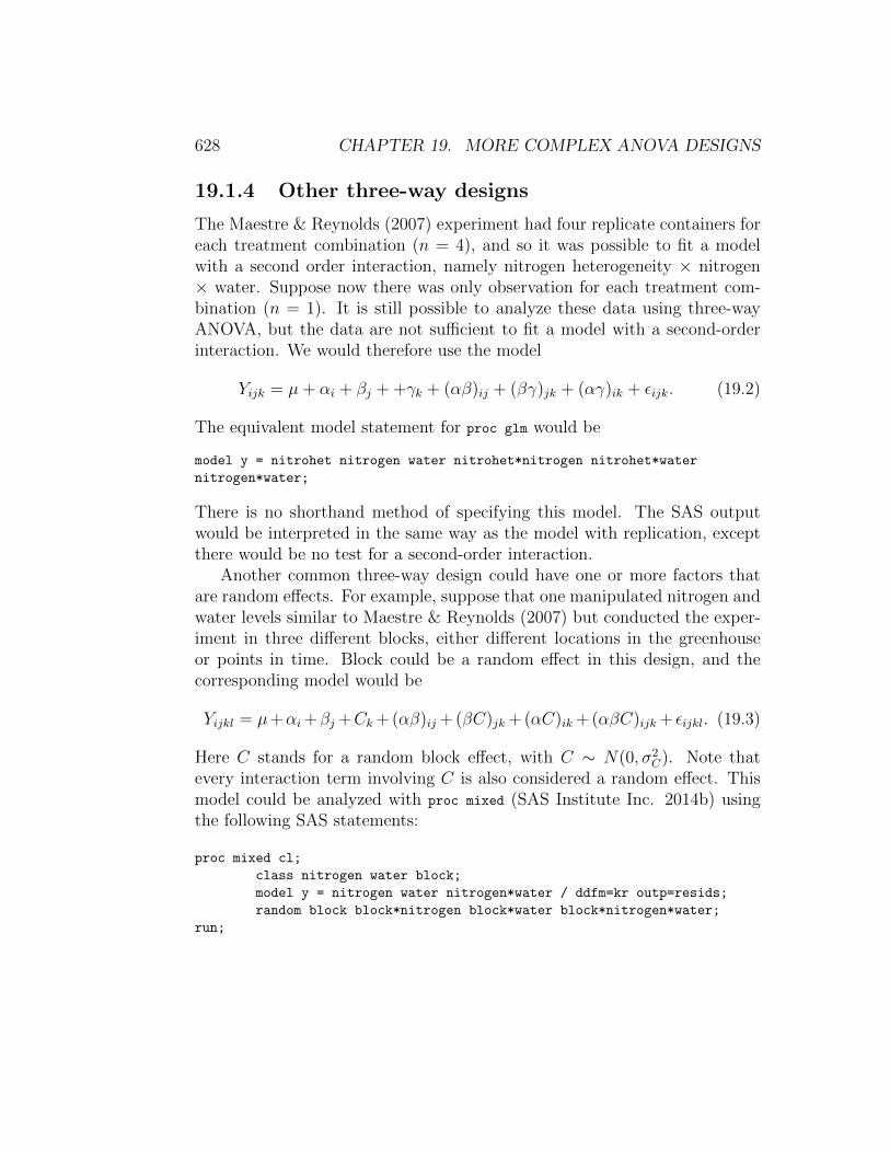
The Maestre & Reynolds (2007) experiment had four replicate containers foreach treatment combination (n = 4), and so it was possible to fit a modelwith a second order interaction, namely nitrogen heterogeneity × nitrogen× water. Suppose now there was only observation for each treatment com-bination (n = 1). It is still possible to analyze these data using three-wayANOVA, but the data are not sufficient to fit a model with a second-orderinteraction. We would therefore use the model
Yijk = µ+ αi + βj + +γk + (αβ)ij + (βγ)jk + (αγ)ik + εijk. (19.2)
The equivalent model statement for proc glm would be
model y = nitrohet nitrogen water nitrohet*nitrogen nitrohet*water
nitrogen*water;
There is no shorthand method of specifying this model. The SAS outputwould be interpreted in the same way as the model with replication, exceptthere would be no test for a second-order interaction.
Another common three-way design could have one or more factors thatare random effects. For example, suppose that one manipulated nitrogen andwater levels similar to Maestre & Reynolds (2007) but conducted the exper-iment in three different blocks, either different locations in the greenhouseor points in time. Block could be a random effect in this design, and thecorresponding model would be
Yijkl = µ+αi +βj +Ck + (αβ)ij + (βC)jk + (αC)ik + (αβC)ijk + εijkl. (19.3)
Here C stands for a random block effect, with C ∼ N(0, σ2C). Note that
every interaction term involving C is also considered a random effect. Thismodel could be analyzed with proc mixed (SAS Institute Inc. 2014b) usingthe following SAS statements:
proc mixed cl;
class nitrogen water block;
model y = nitrogen water nitrogen*water / ddfm=kr outp=resids;
random block block*nitrogen block*water block*nitrogen*water;
run;

19.2. ONE-WAY NESTED ANOVA 629
19.2 One-way nested ANOVA
The second design we will examine are called one-way nested designs. Thereare two factors in this design, a Factor A that may be a fixed or randomeffect, and a random nested Factor B. Nested means that for each level ofFactor A, there are several levels of Factor B that are unique to that level ofA. There are several replicate observations for each combination of Factor Aand B.
As an example of this design, we will examine a genetic study of a minuteparasitic wasp, Anagrus delicatus (Hymenoptera: Mymaridae). This waspattacks eggs of the planthopper Prokelisia marginata (Homoptera: Delphaci-dae), a salt marsh insect that feeds on Spartina plants. Cronin & Strong(1996) were interested in the genetics of various wasp traits, including thenumber of eggs carried by the wasps themselves, ovipositor length, and vari-ous behavioral traits. They collected female wasps from three separate sitesin San Franciso Bay and established genetically identical isolines from in-dividual wasps collected from each site. They then measured the traits fora number of individuals from each isoline. Isolines are the nested factor inthis design, because each isoline was established from a single site. Siteswere classified as a fixed effect because there were essentially only three sitesavailable for sampling, and so the sites were not randomly selected from apopulation of sites. Example 2 below shows a simulated data set based onthis study, with three sites, 14 isolines per site, and eight individuals perisoline.

630 CHAPTER 19. MORE COMPLEX ANOVA DESIGNS
Table 19.2: Example 2 - Fecundity for Anagrus delicatus collected from threedifferent sites, with 14 isolines per site and eight wasps per isoline. The datawere simulated from results presented in Cronin and Strong (1996). Notethat the values in the site, isoline, and wasp columns also correspond to thesubscripts for Yijk. See Chapter 21 for the full version of this data set.
Site Isoline Wasp Yijk = eggs1 1 1 371 1 2 411 1 3 461 1 4 441 1 5 431 1 6 411 1 7 381 1 8 371 2 1 371 2 2 281 2 3 341 2 4 371 2 5 351 2 6 391 2 7 36
etc.
3 13 1 363 13 2 393 13 3 363 13 4 303 13 5 373 13 6 323 13 7 383 13 8 393 14 1 323 14 2 343 14 3 413 14 4 333 14 5 353 14 6 353 14 7 343 14 8 31

19.2. ONE-WAY NESTED ANOVA 631
19.2.1 Nested ANOVA models
Suppose that we want to model the observations in a study like Example 2,where there is a fixed Factor A and a nested Factor B. A common model forthe observations Yijk in such designs (Winer et al. 1991) is
Yijk = µ+ αi +Bj(i) + εijk. (19.4)
Here µ is the grand mean of the observations, αi the deviation from µ causedby the ith level or treatment of Factor A, and Bj(i) the random deviationcaused by the jth level of Factor B within the ith level of Factor A. Bj(i) isassumed to be normally distributed with mean zero and variance σ2
B(A), or
Bj(i) ∼ N(0, σ2B(A)), while εijk ∼ N(0, σ2) as usual. Bj(i) and εijk are assumed
to be independent. This model has two variance components, namely σ2B(A)
and σ2.The behavior of this model is illustrated in Fig. 19.6, for a = 3 levels of
Factor A and b = 4 levels of Factor B nested within A. The figure illustrateshow the value of αi shifts the mean of the observations away from µ, similarto other ANOVA models. The Bj(i) values, which are random variables, shiftthe observations for each nested level away from the values set by µ + αi.Because they are random variables, the values of Bj(i) are different for eachlevel of Factor A.
The usual objectives for this nested ANOVA design are to test for FactorA effects, and estimate the variance components σ2
B(A) and σ2. For Factor Athis amounts to testing H0 : all αi = 0. We will not consider this process indetail but proceed to the analysis and interpretation of the Example 2 dataset. We will use proc mixed for the analysis because this design involves amixed model.

632 CHAPTER 19. MORE COMPLEX ANOVA DESIGNS
Figure 19.6: Mixed model for nested ANOVA showing the Factor A and Beffects.
19.2.2 Nested ANOVA for Example 2 - SAS demo
The first step in analyzing the Example 2 data is to read the observationsusing a data step, with the variables site and isoline denoting the collectionsite and Anagrus isoline (see below). Although the isolines are numberedsimilarly across the three sites, note they are actually unique to each siteand so are nested within sites. The variable wasp refers to a particular waspwithin each isoline, but is not used in the analyses. Two plots are thenrequested using proc gplot (SAS Institute Inc. 2014a), one showing the meanfor each site and so illustrating the site effect. The second plot shows theindividual wasps color-coded by isoline, allowing for a visual comparison ofvariation among and within isolines. The x-axis position of each wasp isjittered to keep the points from overlapping. This involves adding a smallrandom quantity to the site value, generating a new variable called site_jit
that differs for each wasp.The next section of the program conducts the nested ANOVA using
proc mixed (SAS Institute Inc. 2014b). The class statement tells SAS thatsite and isoline are used to classify the observations. Next, the fixed effectsite is listed in the model statement, while the random, nested effect of isoline

19.2. ONE-WAY NESTED ANOVA 633
is incorporated in the random statement. SAS uses the syntax isoline(site)
to indicate that isoline is nested within site. An lsmeans statement is used tocompared the different sites using the Tukey method.
The analysis found no significant effect of site (F2,39 = 2.3, P = 0.1323)on the number of eggs per wasp (Fig. 19.7. The estimated variance amongisolines within sites (σ2
B(A) = σ2site(isoline) = 10.17) was substantial relative
to the variance among wasps within isolines (σ2 = 11.02). This patterncan be observed in Fig. 19.8, with the observations for each isoline fallinginto discernable groups. This suggests that variation in egg number has asignificant genetic component.
We can use the two variance components to estimate the heritability ofegg number, which is the proportion of the variance due to genotypic vs.phenotypic differences among individuals (Falconer & Mackay 1996). Thegenotypic variance, VG, is estimated by the variance among isolines withinsites, because each isoline represents a different genetic group. For the waspexample, we have VG = σ2
site(isoline) = 10.17. The environmental variance, VE,is estimated by the variance among individuals within isolines, and representsvariation among individuals not due to genotype. It is estimated by thevariance among wasps within isolines, or VE = σ2 = 11.02. The phenotypicvariance is defined as the sum of the genotypic and environmental variance,or VP = VG + VE. Heritability is then defined h2 = VG/VP = VG/(VG + VE).It follows that h2 = 10.17/(10.17 + 11.02) = 0.48 for the number of eggs inthe wasps. This is relatively large value, suggesting that egg number couldreadily evolve in response to selection pressure.

634 CHAPTER 19. MORE COMPLEX ANOVA DESIGNS
SAS program
* Nested_ANOVA_Anagrus.sas;
options pageno=1 linesize=80;
goptions reset=all;
title "Nested ANOVA for fecundity";
title2 "Data simulated from Cronin and Strong (1996)";
data anagrus;
input site isoline wasp eggs;
* Apply transformations here;
y = eggs;
* Make jittered data for plots;
site_jit = site + 0.1*rannor(0);
datalines;
1 1 1 37
1 1 2 41
1 1 3 46
1 1 4 44
1 1 5 43
1 1 6 41
1 1 7 38
1 1 8 37
etc.
3 14 1 32
3 14 2 34
3 14 3 41
3 14 4 33
3 14 5 35
3 14 6 35
3 14 7 34
3 14 8 31
;
proc print data=anagrus;
run;
* Plot means and standard errors for each site;
proc gplot data=anagrus;
plot y*site=1 / vaxis=axis1 haxis=axis1;
symbol1 i=std1jmt v=none height=2 width=3;
axis1 label=(height=2) value=(height=2) width=3 major=(width=2) minor=none;
run;
* Plot observations for each site and isoline;
proc gplot data=anagrus;
plot y*site_jit=isoline / vaxis=axis1 haxis=axis1;

19.2. ONE-WAY NESTED ANOVA 635
symbol1 i=none v=dot height=0.5;
axis1 label=(height=2) value=(height=2) width=3 major=(width=2) minor=none;
run;
* Nested ANOVA mixed model;
proc mixed cl data=anagrus;
class site isoline;
model y = site / ddfm=kr outp=resids;
random isoline(site);
* Compare levels of fixed effect using Tukey’s HSD;
lsmeans site / diff=all adjust=tukey cl adjdfe=row;
run;
goptions reset=all;
title "Diagnostic plots to check ANOVA assumptions";
* Plot residuals vs. predicted values;
proc gplot data=resids;
plot resid*pred=1 / vaxis=axis1 haxis=axis1;
symbol1 v=star height=2 width=3;
axis1 label=(height=2) value=(height=2) width=3 major=(width=2) minor=none;
run;
* Normal quantile plot of residuals;
proc univariate noprint data=resids;
qqplot resid / normal waxis=3 height=4;
run;
quit;

636 CHAPTER 19. MORE COMPLEX ANOVA DESIGNS
SAS output
Nested ANOVA for fecundity 1
Data simulated from Cronin and Strong (1996)
10:55 Tuesday, June 11, 2013
Obs site isoline wasp eggs y site_jit
1 1 1 1 37 37 1.10326
2 1 1 2 41 41 0.90939
3 1 1 3 46 46 1.18465
4 1 1 4 44 44 1.12283
5 1 1 5 43 43 1.09742
6 1 1 6 41 41 0.95798
7 1 1 7 38 38 1.11470
8 1 1 8 37 37 0.98907
etc.
329 3 14 1 32 32 2.89845
330 3 14 2 34 34 2.96535
331 3 14 3 41 41 3.02094
332 3 14 4 33 33 2.92618
333 3 14 5 35 35 2.93152
334 3 14 6 35 35 3.01175
335 3 14 7 34 34 3.06111
336 3 14 8 31 31 2.93977
Nested ANOVA for fecundity 8
Data simulated from Cronin and Strong (1996)
10:55 Tuesday, June 11, 2013
The Mixed Procedure
Model Information
Data Set WORK.ANAGRUS
Dependent Variable y
Covariance Structure Variance Components
Estimation Method REML
Residual Variance Method Profile
Fixed Effects SE Method Kenward-Roger
Degrees of Freedom Method Kenward-Roger

19.2. ONE-WAY NESTED ANOVA 637
Class Level Information
Class Levels Values
site 3 1 2 3
isoline 14 1 2 3 4 5 6 7 8 9 10 11 12 13
14
Dimensions
Covariance Parameters 2
Columns in X 4
Columns in Z 42
Subjects 1
Max Obs Per Subject 336
Number of Observations
Number of Observations Read 336
Number of Observations Used 336
Number of Observations Not Used 0
Iteration History
Iteration Evaluations -2 Res Log Like Criterion
0 1 1965.68443676
1 1 1841.14730382 0.00000000
Convergence criteria met.
Nested ANOVA for fecundity 9
Data simulated from Cronin and Strong (1996)
10:55 Tuesday, June 11, 2013
The Mixed Procedure
Covariance Parameter Estimates

638 CHAPTER 19. MORE COMPLEX ANOVA DESIGNS
Cov Parm Estimate Alpha Lower Upper
isoline(site) 10.1664 0.05 6.5003 18.1260
Residual 11.0187 0.05 9.4338 13.0417
Fit Statistics
-2 Res Log Likelihood 1841.1
AIC (smaller is better) 1845.1
AICC (smaller is better) 1845.2
BIC (smaller is better) 1848.6
Type 3 Tests of Fixed Effects
Num Den
Effect DF DF F Value Pr > F
site 2 39 2.13 0.1323
Least Squares Means
Standard
Effect site Estimate Error DF t Value Pr > |t| Alpha
site 1 34.4821 0.9081 39 37.97 <.0001 0.05
site 2 34.2946 0.9081 39 37.77 <.0001 0.05
site 3 32.0982 0.9081 39 35.35 <.0001 0.05
Least Squares Means
Effect site Lower Upper
site 1 32.6454 36.3188
site 2 32.4579 36.1313
site 3 30.2615 33.9349
Differences of Least Squares Means
Standard
Effect site _site Estimate Error DF t Value Pr > |t| Adjustment

19.2. ONE-WAY NESTED ANOVA 639
site 1 2 0.1875 1.2842 39 0.15 0.8847 Tukey
site 1 3 2.3839 1.2842 39 1.86 0.0710 Tukey
Nested ANOVA for fecundity 10
Data simulated from Cronin and Strong (1996)
08:29 Monday, November 11, 2013
The Mixed Procedure
Differences of Least Squares Means
Standard
Effect site _site Estimate Error DF t Value Pr > |t| Adjustment
site 2 3 2.1964 1.2842 39 1.71 0.0951 Tukey
Differences of Least Squares Means
Adj Adj
Effect site _site Adj P Alpha Lower Upper Lower Upper
site 1 2 0.9883 0.05 -2.4100 2.7850 -2.9411 3.3161
site 1 3 0.1651 0.05 -0.2136 4.9814 -0.7447 5.5126
site 2 3 0.2142 0.05 -0.4011 4.7939 -0.9322 5.3251

640 CHAPTER 19. MORE COMPLEX ANOVA DESIGNS
Figure 19.7: Means ± standard errors for each site in the Example 2 study,where Y = eggs.
Figure 19.8: Observations for each site and isoline in the Example 2 study,where Y = eggs.

19.3. ANALYSIS OF COVARIANCE 641
19.3 Analysis of covariance
Analysis of covariance, or ANCOVA, is a design that combines elements ofANOVA and regression. The simplest ANCOVA design is a combination ofone-way ANOVA and linear regression. Factor A in the design is typically afixed effect. For each observation in the design, a covariate X is measuredand along with the dependent variable Y . The covariate X is thought toexplain some level of variation in Y , and by including it in the design thismay increase the power to detect treatment effects. Y is often assumed to belinearly related to X, although nonlinear relationships can be accomodated.More generally, a study might involve a mixture of factors and covariates,and the covariate effects may be of equal or greater interest than the factors.
As an example of ANCOVA, we will analyze a study of the fitness ofadult Thanasimus dubius, a bark beetle predator, reared on an artificial dietvs. individuals collected from the wild (Reeve et al. 2003). The fitnessvariables measured were the total number of eggs laid (fecundity) and elytrallength (Table 19.3). Body size and fecundity are often related in insects, soelytral length was used as a covariate in the analysis. This helps control fornatural variation in body size to better see the treatment effect. The threetreatments in the study were (1) artificial diet as larvae and Ips grandicollisas adults (DietIG), (2) artificial diet and cowpea weevils (DietCPW), and (3)wild adults fed cowpea weevils (WildCPW). The wild adults were collected fromthe field and so reared on natural prey as larvae. We will use the notationYij to reference the observations in ANCOVA designs, with the i subscriptrefering to the Factor A or treatment group, while j is the observation withinthe treatment.

642 CHAPTER 19. MORE COMPLEX ANOVA DESIGNS
Table 19.3: Example 3 - Fitness of the predator T. dubius, reared on anartificial diet as larvae vs. wild individuals collected from the field (Reeve etal. 2003). See Chapter 21 for the full data set.
Yij = Eggs Xij = Length (mm) Treatment i j290 5.7 DietIG 1 199 5.2 DietIG 1 2
340 5.5 DietIG 1 3271 4.8 DietIG 1 4200 5.2 DietIG 1 5
etc.
66 4.6 DietCPW 2 193 5.0 DietCPW 2 29 5.4 DietCPW 2 3
404 5.4 DietCPW 2 4244 5.1 DietCPW 2 5
etc.
62 4.7 WildCPW 3 1290 5.0 WildCPW 3 2488 5.8 WildCPW 3 3336 5.2 WildCPW 3 4337 5.8 WildCPW 3 5
etc.

19.3. ANALYSIS OF COVARIANCE 643
19.3.1 ANCOVA model
The following model is commonly used for simple ANCOVA designs (Wineret al. 1991). We have
Yij = µ+ αi + β(Xij − X) + εij, (19.5)
where µ is the grand mean and αi is the deviation from µ caused by the ithlevel of Factor A. The term Xij is the value of the covariate for observationYij, while X is the average of all the covariate values. The parameter β isthe slope of the relationship between Yij and Xij. This slope is assumed tobe the same across all levels of Factor A. We will later see how to test thisassumption. As usual, the model assumes εij ∼ N(0, σ2).
The model can also be written in the form
Y ′ij = Yij − β(Xij − X) = µ+ αi + εij. (19.6)
Displayed this way, we can see that ANCOVA is equivalent to carrying out aone-way ANOVA on values of Yij that have been adjusted for the covariateX, namely the values of Y ′ij.
Another adjustment of the model is needed by SAS and other statisticalsoftware. Combining some elements, the model can be written as
Yij = µ′ + αi + βXij + εij, (19.7)
where µ′ = µ−βX. The quantity µ′ represents a grand mean adjusted for theeffect of the covariate. The objective in ANCOVA is to test whether FactorA and the covariate have an effect, and so test H0 : all αi = 0 and H0 : β = 0.However, before conducting these F tests we will first test whether the slopesacross Factor A groups are identical by including an interaction term in theSAS model. If the slopes are significantly different, we have a scenario similarto ANOVA when interaction is present (see Chapter 14). Like ANOVA, whenthe interaction is significant tests of the main effects in ANCOVA, namelyFactor A and the covariate X, may not make sense.
19.3.2 ANCOVA for Example 3 - SAS demo
The first step in the analysis (see program below) is to plot the number ofeggs (y) for each treatment (treat) against elytral length, the covariate (x),using proc gplot (SAS Institute Inc. 2014a). This gives some idea whether

644 CHAPTER 19. MORE COMPLEX ANOVA DESIGNS
each treatment group has the same slope, a key assumption of ANCOVA.The slopes do appear to be similar (Fig. 19.9).
We then fit the ANCOVA model using proc glm, because all the effectsin the model are fixed effects (SAS Institute Inc. 2014b). The first step isto fit a model with an interaction between the treatment and covariate, andexamine the test for the interaction (see first SAS output below). We see thatit is non-significant (F2,35 = 0.02, P = 0.9781), and so can assume the slopesare the same across treatments. We then rerun the program using the modelwithout interaction. We see a highly significant effect of the covariate (F1,37 =9.99, P = 0.0031), illustrating the typical strong relationship between bodysize and fecundity in insects. The treatment effect was nonsigificant (F2,37 =0.52, P = 0.5976), implying the treatments themselves had no effect on eggnumbers. Predators reared on the artificial diet are apparently similar towild predators on this measure of fitness, controlling for elytral length andso body size.
The program also includes an lsmeans statement to calculate the leastsquares means for each treatment group, and test for differences among themusing the Tukey method. Least squares means are means adjusted for theeffect of other variables in the model, and in the case of ANCOVA are thetreatment means adjusted for the covariate. In particular, they have theform
Yi(adj) = Yi − β(Xi − ¯X). (19.8)
We can see they are composed of two terms, the treatment means and theadjustment for the covariate. Treatment groups that have covariate means(Xi values) far from the overall covariate mean ( ¯X) receive a larger adjust-ment. No significant differences were found among the treatment groups,which is not surprising given the overall treatment effect was nonsignificant.
19.3. ANALYSIS OF COVARIANCE 645
SAS Program
* ANCOVA_fitness.sas;
options pageno=1 linesize=80;
goptions reset=all;
title ’ANCOVA for T. dubius fitness’;
data fitness;
input eggs length treat $;
* Choose y and x variables;
y = eggs;
x = length;
datalines;
290 5.7 DietIG
99 5.2 DietIG
340 5.5 DietIG
271 4.8 DietIG
200 5.2 DietIG
etc.
;
run;
* Print data set;
proc print data=fitness;
run;
* Plot data and regression line;
proc gplot data=fitness;
plot y*x=treat / vaxis=axis1 haxis=axis1 legend=legend1;
symbol1 i=rl v=star height=2 width=3;
axis1 label=(height=2) value=(height=2) width=3 major=(width=2) minor=none;
legend1 label=(height=2) value=(height=2);
run;
* ANCOVA;
proc glm data=fitness;
class treat;
* Model with interaction;
*model y = treat x treat*x;
* Model without interaction;
model y = treat x;
lsmeans treat / pdiff=all adjust=tukey cl lines;
output out=resids p=pred r=resid;
run;
goptions reset=all;
title "Diagnostic plots to check ANCOVA assumptions";
* Plot residuals vs. predicted values;

646 CHAPTER 19. MORE COMPLEX ANOVA DESIGNS
proc gplot data=resids;
plot resid*pred=1 / vaxis=axis1 haxis=axis1;
symbol1 v=star height=2 width=3;
axis1 label=(height=2) value=(height=2) width=3 major=(width=2) minor=none;
run;
* Normal quantile plot of residuals;
proc univariate noprint data=resids;
qqplot resid / normal waxis=3 height=4;
run;
quit;
Figure 19.9: Eggs laid by adult T. dubius in three treatments vs. elytralength.

19.3. ANALYSIS OF COVARIANCE 647
SAS Output - Model with Interaction
ANCOVA for T. dubius fitness 3
13:26 Thursday, September 26, 2013
The GLM Procedure
Dependent Variable: y
Sum of
Source DF Squares Mean Square F Value Pr > F
Model 5 149241.7740 29848.3548 2.13 0.0845
Error 35 489963.3479 13998.9528
Corrected Total 40 639205.1220
R-Square Coeff Var Root MSE y Mean
0.233480 47.29918 118.3172 250.1463
Source DF Type I SS Mean Square F Value Pr > F
treat 2 16193.0211 8096.5105 0.58 0.5661
x 1 132427.1693 132427.1693 9.46 0.0041
x*treat 2 621.5837 310.7918 0.02 0.9781
Source DF Type III SS Mean Square F Value Pr > F
treat 2 396.6464 198.3232 0.01 0.9859
x 1 114086.8726 114086.8726 8.15 0.0072
x*treat 2 621.5837 310.7918 0.02 0.9781

648 CHAPTER 19. MORE COMPLEX ANOVA DESIGNS
SAS Output - Model without Interaction
ANCOVA for T. dubius fitness 1
08:29 Monday, November 11, 2013
Obs eggs length treat y x
1 290 5.7 DietIG 290 5.7
2 99 5.2 DietIG 99 5.2
3 340 5.5 DietIG 340 5.5
4 271 4.8 DietIG 271 4.8
5 200 5.2 DietIG 200 5.2
etc.
ANCOVA for T. dubius fitness 2
08:29 Monday, November 11, 2013
The GLM Procedure
Class Level Information
Class Levels Values
treat 3 DietCPW DietIG WildCPW
Number of Observations Read 41
Number of Observations Used 41
ANCOVA for T. dubius fitness 3
08:29 Monday, November 11, 2013
The GLM Procedure
Dependent Variable: y
Sum of
Source DF Squares Mean Square F Value Pr > F
Model 3 148620.1904 49540.0635 3.74 0.0193
Error 37 490584.9316 13259.0522

19.3. ANALYSIS OF COVARIANCE 649
Corrected Total 40 639205.1220
R-Square Coeff Var Root MSE y Mean
0.232508 46.03224 115.1480 250.1463
Source DF Type I SS Mean Square F Value Pr > F
treat 2 16193.0211 8096.5105 0.61 0.5484
x 1 132427.1693 132427.1693 9.99 0.0031
Source DF Type III SS Mean Square F Value Pr > F
treat 2 13846.2749 6923.1375 0.52 0.5976
x 1 132427.1693 132427.1693 9.99 0.0031
ANCOVA for T. dubius fitness 4
08:29 Monday, November 11, 2013
The GLM Procedure
Least Squares Means
Adjustment for Multiple Comparisons: Tukey-Kramer
LSMEAN
treat y LSMEAN Number
DietCPW 270.496170 1
DietIG 221.056056 2
WildCPW 251.610513 3
Least Squares Means for effect treat
Pr > |t| for H0: LSMean(i)=LSMean(j)
Dependent Variable: y
i/j 1 2 3
1 0.5702 0.8992
2 0.5702 0.7839

650 CHAPTER 19. MORE COMPLEX ANOVA DESIGNS
3 0.8992 0.7839
treat y LSMEAN 95% Confidence Limits
DietCPW 270.496170 205.021331 335.971009
DietIG 221.056056 147.207956 294.904156
WildCPW 251.610513 195.890594 307.330433
Least Squares Means for Effect treat
Difference Simultaneous 95%
Between Confidence Limits for
i j Means LSMean(i)-LSMean(j)
1 2 49.440114 -69.094011 167.974239
1 3 18.885656 -85.958935 123.730248
2 3 -30.554457 -142.397015 81.288100
Tukey-Kramer Comparison Lines for Least Squares Means of treat
LS-means with the same letter are not significantly different.
LSMEAN
y LSMEAN treat Number
A 270.496 DietCPW 1
A
A 251.611 WildCPW 3
A
A 221.056 DietIG 2

19.4. REFERENCES 651
19.4 References
Cronin, J. T. & Strong, D. R. (1996) Genetics of oviposition success of athelytokous fairyfly parasitoid, Anagrus delicatus. Heredity 76: 43-54.
Falconer, D. S. & MacKay, T. F. C. (1996) Introduction to QuantitativeGenetics, 4th edition. Longman Group Ltd., Essex, England.
Maestre, F. T. & Reynolds, J. F. (2007) Amount or pattern? Grassland re-sponses to the heterogeneity and availability of two key resources. Ecology88: 501-511.
Reeve, J. D., Rojas, M. G. & Morales-Ramos, J. A. (2003) Artificial dietand rearing methods for Thanasimus dubius (Coleoptera: Cleridae), apredator of bark beetles (Coleoptera: Scolytidae). Biological Control 27:315-322.
SAS Institute Inc. (2014a) SAS/GRAPH 9.4: Reference, Third Edition.SAS Institute Inc., Cary, NC.
SAS Institute Inc. (2014b) SAS/STAT 13.2 Users Guide. SAS Institute Inc.,Cary, NC.
Winer, B. J., Brown, D. R. & Michels, K. M. (1991) Statistical Principles inExperimental Design, 3rd edition. McGraw-Hill, Inc., Boston, MA.

652 CHAPTER 19. MORE COMPLEX ANOVA DESIGNS
19.5 Problems
1. A limnologist wants to examine the length of a zooplankton speciesreared using four different algal growth media (1, 2, 3, and 4). Sheis also interested in whether there is variation among the containersused to rear the organisms. An experiment is conducted where threecontainers are used for each rearing medium, for a total of 12 differentcontainers. The containers were randomly selected from a box of con-tainers. The length of four animals was determined for each container,yielding the following data:
Medium Container Lengths 1-4 (mm)1 1 3.1, 3.0, 3.2, 3.01 2 3.3, 3.6, 2.8, 2.51 3 3.7, 3.4, 3.4, 3.62 1 2.7, 2.9, 3.2, 3.02 2 2.9, 3.4, 3.5, 2.92 3 3.5, 3.5, 3.7, 4.03 1 2.8, 2.7, 1.8, 2.53 2 2.6, 2.5, 3.2, 2.43 3 2.6, 2.9, 1.8, 2.44 1 4.1, 4.6, 3.3, 4.54 2 3.7, 3.9, 4.0, 3.94 3 4.4, 4.4, 3.9, 4.6
(a) Write an appropriate ANOVA model for this design, stating whichfactors are fixed, random, and possibly nested.
(b) Use SAS to analyze these data using your ANOVA model, trans-forming the observations only if necessary. Is there a significantdifference among the four media in zooplankton length?
(c) Use the Tukey method to compare the media treatments. Inter-pret your results.
(d) Compare the magnitude of your variance components. Does thereappear to be much variation among containers?
2. An ecologist is interested in the effect of three management treatments(labeled 1, 2, and 3) on the abundance of an endangered snail. Treat-ment 2 is a control treatment. Twenty-four plots are established and

19.5. PROBLEMS 653
the three treatments assigned at random to the plots. The density ofsnails is then measured at a later time, as well as a covariate in theform of a habitat index. Larger values of the habitat index are thoughtto indicate better snail habitat. See data set below.
Treatment Index Snails1 9.3 23.01 9.8 24.91 9.9 24.71 10.1 24.61 8.9 23.41 10.8 27.11 9.6 25.41 10.7 25.42 11.9 21.82 9.6 18.82 10.3 21.02 10.8 21.52 9.9 20.92 10.9 22.62 8.9 19.82 10.2 22.43 11.2 23.43 10.3 18.53 11.1 22.33 9.8 20.53 11.2 20.53 8.7 18.43 8.4 18.73 10.5 19.2
(a) Test for equality of slopes among the different treatment groupsusing SAS. Is this key assumption of ANCOVA satisfied?
(b) Use ANCOVA and SAS to test for overall treatment and covariateeffects in this experiment, and the Tukey method to compare thedifferent treatments. Interpret and discuss your results. Is therea significant treatment and covariate effect? How do the differenttreatments compare?

654 CHAPTER 19. MORE COMPLEX ANOVA DESIGNS
3. A scientist interested in aquaculture raises fish using three kinds oftreatments in a factorial design. There were two fish diets (A and B),two strains of fish (1 and 2), and three temperatures (22o, 24o, and26oC). Two fish were reared for each combination of the treatments.The following data were obtained:
Diet Strain Temp Weight (lb)A 1 22 5.5A 1 22 5.8A 1 24 5.9A 1 24 5.7A 1 26 6.2A 1 26 5.9A 2 22 5.2A 2 22 5.0A 2 24 5.4A 2 24 5.6A 2 26 5.0A 2 26 4.9B 1 22 5.4B 1 22 4.8B 1 24 5.4B 1 24 5.4B 1 26 5.7B 1 26 5.5B 2 22 5.2B 2 22 4.8B 2 24 5.1B 2 24 5.1B 2 26 4.8B 2 26 4.5
(a) Write an appropriate ANOVA model for this design, stating whichfactors are fixed or random.
(b) Use SAS to analyze these data using your ANOVA model, trans-forming the observations only if necessary. Interpret the results ofyour analysis.