Default Bayes Factors for ANOVA Designs

Jeffrey N. Roudera,∗, Richard D. Moreyb, Paul L. Speckmanc, Jordan M.Provincea

aDepartment of Psychological Sciences, University of MissouribFaculty of Behavioural and Social Sciences, University of Groningen

cDepartment of Statistics, University of Missouri

Abstract

Bayes factors have been advocated as superior to p-values for assessing sta-tistical evidence in data. Despite the advantages of Bayes factors and thedrawbacks of p-values, inference by p-values is still nearly ubiquitous. Oneimpediment to adoption of Bayes factors is a lack of practical development,particularly a lack of ready-to-use formulas and algorithms. In this paper,we discuss and expand a set of default Bayes factor tests for ANOVA de-signs. These tests are based on multivariate generalizations of Cauchy priorson standardized effects, and have the desirable properties of being invariantwith respect to linear transformations of measurement units. Moreover, theseBayes factors are computationally convenient, and straightforward samplingalgorithms are provided. We cover models with fixed, random, and mixedeffects, including random interactions, and do so for within-subject, between-subject, and mixed designs. We extend the discussion to regression modelswith continuous covariates. We also discuss how these Bayes factors maybe applied in nonlinear settings, and show how they are useful in differen-tiating between the power law and the exponential law of skill acquisition.In sum, the current development makes the computation of Bayes factorsstraightforward for the vast majority of designs in experimental psychology.

∗Correspondence: 210 McAlester Hall, Columbia, MO 65203, rouderj@missouri.edu.We thank Brandon Turner and Eric-Jan Wagenmakers for detailed and constructive com-ments. This research is supported by NSF SES 1024080.

Preprint submitted to Elsevier August 3, 2012

1. Introduction

Psychological scientists routinely use data to inform theory. It is commonto report p-values from t-tests and F -tests as evidence favoring certain the-oretical positions and disfavoring others. There are a number of critiques ofthe use of p-values as evidence, and we join a growing chorus of researcherswho advocate the Bayes factor as a measure of evidence for competing posi-tions (Edwards et al., 1963; Gallistel, 2009; Kass, 1992; Myung & Pitt, 1997;Raftery, 1995; Rouder et al., 2009; Wagenmakers, 2007). Even though manyof us are convinced that Bayes factor is intellectually more appealing thatinference by p-values, there is a pronounced lack of detailed development ofBayes factors for real-world experimental designs common in psychologicalscience. Perhaps the problem can be illustrated by a recent experience of thefirst author. After giving a colloquium talk comparing Bayes factors to p-values, he was approached by an excited colleague asking for help computinga Bayes factor for a run-of-the-mill three-way ANOVA design. At the time,the first author did not know how to compute this Bayes factor. After all,there were no books that covered it, and the computation was not built intoany commonly-used software.

Although the Bayes factor is conceptually straightforward, the computa-tion requires a specification of priors over all parameters and an integrationof the likelihood with respect to these priors. Useful priors should exhibittwo general properties: First, they should be judiciously chosen because theresulting Bayes factors depends to some degree on the prior. Second, theyshould be computationally convenient so that the integration of the likeli-hood is stable and relatively fast. Showing that the priors are judicious andconvenient entails much development. Substantive researchers typically haveneither the skills nor the time to develop Bayes factors for their own choiceof priors. To help mitigate this problem, we provide default priors and asso-ciated Bayes factors for common research designs. These default priors aregeneral, broadly applicable, computationally convenient, and lead to Bayesfactors that have desirable theoretical properties. The defaults priors maynot be the best choice in all circumstances, but they are reasonable in most.

The topic in this paper is the development of default Bayes factors forthe linear model underlying ANOVA and regression. In experimental psy-chology there is a distinction between linear models, which are used to assessthe effects of manipulations, and domain-specific models of psychologicalprocesses. Linear models are simple and broadly applicable, whereas pro-

2

cess models are typically nonlinear, complex, and targeted to explore specificphenomena, processes, or paradigms. In many cases, an ultimate goal isthe development of Bayes factor methods for comparing competing processmodels. Given this distinction and the appeal of process models, it mayseem strange that the majority of the development here is for linear models.There are three advantages to this development: First, ANOVA and regres-sion are still the most popular tests in experimental psychology. Develop-ing Bayes factors for these models is a necessary precursor for widespreadadoption of the method. In this paper we provide development for manyANOVA designs, including within-subject, between-subject and mixed de-signs. Second, many nonlinear models have linear subcomponents. Linearsubcomponents may be used to account for nuisance variation in the sam-pling of participants or items. For example, Pratte & Rouder (2011) fitYonelinas’ dual process recognition-memory model (Yonelinas, 1999) to real-world recognition-memory data where each observation comes from a uniquecross of people and items. To fit the model, Pratte and Rouder placed addi-tive linear models on critical mnemonic parameters that incorporated peopleand items as additive random effects. In cases such as this, development ofBayes factors for inference with linear models is a natural precursor to devel-opment for nonlinear models. Third, the priors suggested here may transferwell to nonlinear cases. We provide an example of this transfer by developingBayes factors to test between the power law and the exponential law of skillacquisition.

This paper is organized as follows. In the next section, we review com-mon critiques of null hypothesis significance testing, which lead naturally toconsideration of the Bayes factor. In Section 3, the Bayes factor is presented,along with a discussion of how it should be interpreted when assessing theevidence from data for competing positions. Following this discussion, wediscuss the properties of good default priors, and provide default priors forthe one-sample case. These existing default priors are then generalized forseveral effects in Section 5 and 6. In Section 7 and 8, we present Bayes fac-tors for one-way and multi-way ANOVA, respectively, for both random andfixed effects. In Section 9, we discuss how within-subject, between-subjectand mixed designs may be analyzed. In Section 10 we provide an examplefrom linguistics that is known to be particularly problematic. In linguis-tic designs, both items and participants should be treated simultaneouslyas random effects, and failure to do so substantially affects the quality ofinference (Clark, 1973). We show how this treatment may be accomplished

3

in a straightforward fashion with the developed Bayes factor methodology.Sections 11 through 14 provide discussion about the large-sample propertiesof the Bayes factors, alternative choices for priors, solutions for regression de-signs, and a discussion of computational issues, respectively. In Section 15,we discuss how the developed priors may be extended for nonlinear cases,and provide an example in assessing learning curves.

2. Critiques of Significance Testing

It has often been noted that there is a fundamental tension between nullhypothesis significance testing and the goals of science. On the one hand,researchers seek simplicity or parsimony to explain target phenomena. Anexample of such simplicity comes from the work of Gilovich et al. (1985), whoassessed whether basketball shooters display hot and cold streaks in whichthe outcome of one shot attempt affects the outcome of subsequent ones.They concluded that there was no such dependency, which is a conclusion infavor of simplicity over complexity. In null hypothesis significance tests, thesimpler model which serve as nulls may only be rejected and never affirmed.Hence, researchers using significance testing find themselves on the “wrongside” of the null hypothesis whenever they argue for the null hypothesis. Ifthe null is true, the best case outcome of a significance test is a statementabout a lack of evidence for an effect. It would be desirable to state positiveevidence for a lack of an effect.

Being on the wrong side of the null is not rare. Other examples includetests of subliminal perception (perception must be shown to be at chance lev-els, e.g., Dehaene et al., 1998; Murphy & Zajonc, 1993), expectancies of anequivalence of performance across group membership (such as gender, e.g.,Shibley Hyde, 2005), or assessment of a lack of interaction between factors(e.g., Sternberg, 1969). Additionally, models that predict stable relation-ships, such as the Fechner-Weber Law1, serve as null hypotheses. Researcherswho test strong theoretical positions that predict specified invariances or reg-ularities in data are typically on the wrong side of the null. From a theoreticalpoint of view, being on the wrong side of the null is an enviable position:

1The Fechner-Weber Law (Fechner, 1966; Masin et al., 2009) describes how bright aflash must be to be detected against a background. If the background has intensity I, theflash must be of intensity I(1 + θ) to be detected. The parameter θ, the Weber fraction,is posited to remain invariant across different background intensities.

4

the goal of scientific theory is often to model or explain observed invariances.Testing strong invariances often indicates a high level of theoretical sophis-tication. From a practical point of view, however, being on the wrong sideof the null presents statistical difficulties. This tension, that null hypothesesare theoretically desirable yet are impossible to support by significance test-ing, has been noted repeatedly (Gallistel, 2009; Kass, 1992; Raftery, 1995;Rouder et al., 2009).

The asymmetry in significance testing in which the null may be rejectedbut not supported is a staple of introductory statistics courses. Yet, it has asubtle but pervasive implication that is often overlooked: significance testsoverstate the case against the null (Berger & Berry, 1988; Edwards et al.,1963; Wagenmakers, 2007). This bias is highly problematic because it meansthat researchers may reject the null without substantial evidence against it.The following argument, adapted from Sellke et al. (2001), demonstratesthis bias. Consider the distributions of p-values under competing hypotheses(Figure 1A). If the null hypothesis is false, then p-values tend to be small, anddecrease (in distribution) as sample size increases. The dashed line coloredgreen shows the distribution of p-values when the underlying effect size is .2and the sample size is 50; the dashed-dotted line colored red shows the samewhen the sample size is increased to 500. The distribution of p-values underthe null, however, is quite different. Under the null, all p-values are equallylikely (solid line colored blue in Figure 1A). This uniform distribution underthe null hypothesis holds regardless of sample size.

If the null is rejected by significance testing, then, presumably, the ob-served data are more improbable under the null than under some other pointalternative. A reasonable measure of evidence is the factor by which the dataare more probable under this alternative than under the null. Suppose a dataset with sample size of 50 yields a p-value in the interval between .04 and.05, which is sufficiently small by convention to reject the null hypothesis.Figure 1B shows the distributions of p-values around this interval for thenull and the alternative that the effect size = .2. The probabilities that thep-value will fall in the interval are represented by the shaded areas under thecurves, which are .01 and .04 under the null and alternative hypotheses, re-spectively. The ratio is .04/.01 = 4: The probability of the observed p-valueis four times more likely under the alternative than under the null. Althoughsuch a ratio constitutes evidence for the alternative, it is not as substantialas might be mistakenly inferred by the fact that the p-value is less than .05.

Figure 1C shows a similar plot for the null and alternative (effect size = .2)

5

0.0 0.2 0.4 0.6 0.8 1.0

05

1015

p−Value

Den

sity

Alt: 50Alt: 500Null

A.

0.00 0.02 0.04 0.06 0.08

01

23

45

p−Value

Den

sity

Alt: 50Null

B.

0.00 0.02 0.04 0.06 0.08

01

23

45

p−Value

Den

sity

Alt: 500Null

C.

The Alternative (probability correct)

Pro

babi

lity

Rat

io

0.50 0.52 0.54 0.56 0.58 0.60

1e−

040.

011

1010

00

●

D.

Figure 1: Significance tests overstate the evidence against the null hypothesis. A. Thedistribution of p-values for an alternative with effect-size of .2 (dashed and dashed-dottedlines are for sample sizes of 50 and 500, respectively) and the null (solid line). B. Prob-ability of observing a p-value between .04 and .05 for the alternative (effect size = .2)and null for N = 50. The probability favors the alternative by a ratio of about 4 to 1.C. Probability of observing a p-value between .04 and .05 for the alternative (effect size= .2) and null for N = 500. The probability favors the null by a factor of 10. D. Theprobability ratio as a function of alternative. The probability ratio is the probability ofobserving a t-value of 2.51 and N = 100 given an alternative divided by the probability ofobserving this t-value for N = 100 given the null. The circle and square points highlightalternatives for which the ratios favor the alternative and null, respectively.6

for a large sample size of 500. For this effect size and sample size, very smallp-values are the norm. Let’s again suppose we observe a p-value between.04 and .05, which leads conventionally to a rejection of the null hypothesis.The probability of observing this p-value under the null remains at .01. Butthe probability of observing it under the alternative with such a large samplesize is close to .001. Therefore, observing a p-value between .04 and .05is about ten times more likely under the null than under the alternative.2

This behavior of significance testing in which researchers reject the null eventhough the evidence overwhelmingly favors it is known as Lindley’s paradox(Lindley, 1957), and is a primary critique of inference by p-values in thestatistical literature.

In Figures 1B and 1C, we compared the evidence for the null againstan alternative in which the effect size under the alternative was a specificvalue (.2). One could ask about these probability ratios for other effect sizes.Consider a recent study of Bem (2011), who claims that people may feel orsense future events that could not be known without psychic powers. In hisExperiment 1, Bem asks 100 participants to guess which of two erotic pictureswill be shown at random, and finds participants have an accuracy of .531,which is significantly above the chance baseline value of .50 (t(99) = 2.51;p < .007). Such small p-values are conventionally interpreted as sufficientevidence to reject the null. Figure 1D, solid line, shows probability that thep-value falls between .0065 and .0075 under a specific alternative relative tothat under the null. These ratios vary greatly with the choice of alternative.Alternatives that are very near the null hypothesis of .5 – say, .525 – arepreferred over the null (filled circle in Figure 1D). Alternatives further from.5, say .58 (filled square) are definitely not preferred over the null. Note thateven though the null is rejected at p = .007, there is only a small range ofalternatives where the probability ratio exceeds 10, and for no alternativedoes it exceed 25, much less 100 (as might naively be inferred from a p-valueless than .01). We see that the null may be rejected by p-values even when theevidence for every specific point alternative is more modest. Note that thecritique that p-values overstate the evidence is not dependent on a Bayesianperspective, and that the probabilities and probability ratios in Figure 1 areused as measures of evidence within the frequentist paradigm, where they

2More generally, a p-value at any nonzero point, say .05, constitutes increasing evidencefor the null in the large sample-size limit.

7

are called likelihood ratios (Hacking, 1965; Royall, 1997).

3. The Bayes Factor

The probability ratio in Figure 1D can be generalized to the Bayes factoras follows. Let B01 denote the Bayes factor between Models M0 and M1.For discretely distributed data,

B01 =Pr(Data|M0)

Pr(Data|M1).

For continuously-distributed data, these probabilities are replaced with prob-ability densities. We use the term probability loosely in the developmentto refer either to probability mass or to probability density, depending onwhether the data are discrete or continuous. We use subscripts on Bayesfactors to refer to the models begin compared, with the first and secondsubscript referring to the model in the numerator and denominator, respec-tively. Accordingly, the Bayes factor for the alternative relative to the nullis denoted B10, B10 = 1/B01.

When models are parameterized,

B01 =

∫θ∈Θ0

Pr(Data|M0,θ)π0(θ)dθ∫θ∈Θ1

Pr(Data|M1,θ)π1(θ)dθ,

where Θ0 and Θ1 are the parameter spaces for Models M0 and M1, re-spectively, and π0 and π1 are the prior probability density functions of theparameters for the respective models. These priors describe the researcher’sprior belief or uncertainty about the parameters. The specification of priorsis critical to defining models, and is the point where subjective probabilityenters the computation of Bayes factor. The argument for subjective prob-ability is made most elegantly in the psychological literature by Edwards etal. (1963), to whom we refer the interested reader. Readers interested in theaxiomatic foundations of subjective probability are referred to Cox (1946),de Finetti (1992), and Jaynes (1986). The numerator and denominator arealso called the marginal likelihoods as they are the integral of the likelihoodfunctions with respect to the priors.

8

Bayes factors describe the relative probability of data under competingpositions. In Bayesian statistics, it is possible to evaluate the relative oddsof the positions themselves, conditional on the data:

Pr(M0|Data)

Pr(M1|Data)= B01 ×

Pr(M0)

Pr(M1),

where the Pr(M0|Data)/Pr(M1|Data) and Pr(M0)/Pr(M1) are posteriorand prior odds, respectively. The prior odds describe the beliefs about themodels before observing the data. The Bayes factor, then, describes how theevidence from the data should change beliefs. For example, a Bayes factor ofB01 = 100 indicates that posterior odds should be 100 times more favorableto the alternative than the prior odds.

The distinction between prior odds, posterior odds and Bayes factors pro-vides an ideal mechanism for adding value to findings. Researchers shouldreport the Bayes factor, and readers can update their own priors accordingly(Jeffreys, 1961; Good, 1979). Sophisticated researchers may add guidanceand value to their analysis by suggesting prior odds, or ranges of prior odds.We use prior odds to add context to our Bayes factor analysis of Bem’s (2011)claim of extrasensory perception of future events that cannot otherwise beknown (Rouder & Morey, 2011). Our Bayes factor analysis of Bem’s datayielded a Bayes factor of 40 in favor of an effect consistent with ESP. We cau-tioned readers, however, to hold substantially unfavorable prior odds towardESP as there is no proposed mechanism, and its existence runs contrary towell-established principles in physics and biology. We believe that a Bayesfactor of 40 is too small to sway readers who hold appropriately skepticalprior odds. Of course, a Bayes factor of 40 may be more consequential in lesscontroversial domains where prior odds are less extreme.

Because Bayes factors measure the evidence for competing positions, theyhave been recommended for inference in psychological settings (an incompletelist includes Edwards et al., 1963; Gallistel, 2009; Lee & Wagenmakers, 2005;Mulder et al., 2009; Rouder et al., 2009; Vanpaemel, 2010; Wagenmakers,2007). There are, however, other Bayesian approaches to inference includingAitkin’s (1991, see Liu & Aitkin, 2008) posterior Bayes factors, Kruschke’s(2010) use of posterior distributions on contrasts, and Gelman and colleagues’notion of model checking through predictive posterior p-values (e.g., Gelmanet al., 2004). The advantages and disadvantages of these methods remainan active and controversial topic in the statistical and social-science method-ological literatures. Covering this literature is outside the scope of this paper,

9

and the interested reader is referred elsewhere: good reviews include Aitkin(1991, especially the subsequent comments), Berger & Sellke (1987, especiallythe subsequent comments), Raftery (1995), and, more recently, Gelman andShalizi (in press). Our view is that none of these alternative approaches offersthe ability to state evidence for invariances and effects in as convincing andas clear a manner as does Bayes factors. Additional discussion is providedin the Conclusion as well as in Morey et al. (in press) and Rouder & Morey(2012).

4. One-Sample Designs

4.1. Model and Priors

In this section, we develop default priors for a one-sample design as anintermediate step toward developing Bayes factors for ANOVA designs. Thedevelopment in this section will be directly relevant throughout. In a one-sample design, there is a single population, and the researcher’s question ofinterest is whether the mean of that population is zero. An example of a one-sample design is a pretest-intervention-posttest design (Campbell & Stanley,1963) in which the researcher tracks each individual’s change between thepretest and posttest. The question of whether the mean intervention effect iszero is typically assessed via consideration of a p-value from a paired-samplet-test. The observed intervention effects are modeled as independent andidentically distributed random variables:

yiiid∼ Normal(µ, σ2), i = 1, . . . , N.

The null model, that there is no treatment effect, is given by µ = 0. To com-pute a Bayes factor, we must also choose a prior distribution for µ under thealternative. It may seem desirable to make µ arbitrarily diffuse to approx-imate a state of minimal prior knowledge. This choice, however, is unwise.Diffuse priors imply that all values are equally plausible, including those thatare obviously implausible. For instance, under a diffuse prior, an effect of5% is as plausible as an effect of one million percent. When the likelihoodunder the alternative is averaged over large, implausible values, the averageapproaches zero. Hence, arbitrarily diffuse priors lead to the result that thenull is more probable than the alternative regardless of the data (Lindley,1957).

10

Jeffreys (1961) recommends reparameterizing the problem in terms ofeffect size, which is denoted by δ, where δ = µ/σ is a dimensionless quantity.The model may then be rewritten:

yi ∼ Normal(σδ, σ2).

Null and alternative models differ in the choice of priors on δ:

M0 : δ = 0,

M1 : δ ∼ Cauchy,

where the Cauchy is a distribution with probability density function

π(x) =1

(1 + x2) π, (1)

and π in the denominator on the right-hand side is the common mathemat-ical constant. Additional details about the Cauchy distribution are providedin Johnson et al. (1994).

Priors must be specified for the remaining parameter in the model, σ2.Fortunately, because this parameter plays an analogous role in bothM0 andM1, it is possible and desirable to place a noninformative Jeffreys prior onσ2:

π(σ2) ∝ 1

σ2.

Bayarri & Garcia-Donato (2007) call this combination of priors the JZS priorsin recognition of the contributions of Jeffreys (1961) as well as Zellner andSiow (1980), who generalized these priors for linear models. The resultingBayes factor, called the JZS Bayes factor, is

B01(t, N) =

(1 + t2

N−1

)−N/2∫ ∞0

(1 +Ng)−1/2(

1 +t2

(1 +Ng)(N − 1)

)−N/2π(g)dg

, (2)

where π(g) is the probability density function of the inverse χ2 distributionwith one degree of freedom:

π(g) = (2π)−1/2g−3/2e−1/(2g). (3)

11

The expression is convenient because the data enter only though the teststatistic t = y

√N/sy, where y and sy are the sample mean and sample

standard deviation of the data, respectively. Fortunately, the expression iscomputationally convenient as the integration is across a single dimensionand may be performed quickly and accurately using Gaussian quadrature(Press et al., 1992). Rouder et al. (2009) provide a web applet for computingthe JZS Bayes factor at pcl.missouri.edu/bayesfactor.

4.2. Properties of the Bayes Factor

Some of the characteristic differences between inference by Bayes factorand p-values are shown in Figure 2. Figure 2A shows the needed t-valuefor stating particular levels of evidence for an effect. Consider the line fora Bayes factor of B10 = 3, which indicates that the data are three timesmore likely under the alternative than under the null. First, note that largert-values are needed to maintain a B01 = 3 than are needed to maintain ap = .05 criterion. Second, note that as the sample size becomes large, in-creasingly larger t-values are needed to maintain the same level of evidence.The need for increasing t-values contrasts with inference by p-values. Fig-ure 2B shows the practical consequences of these different characteristics.The figure summarizes the findings of Wetzels et al. (2011), who providedp-values and JZS Bayes factors for all 855 t-tests reported in the Journalof Experimental Psychology: Learning, memory, and Cognition and Psycho-nomic Bulletin & Review in 2007. We have plotted the results for the 440tests that have p-values between .001 and .15. The plot shows that althoughBayes factors and p-values rely on the same information in the data, theyare calibrated differently. In particular, the tendency of p-values to overstatethe evidence in data against the null hypothesis is apparent. For example, ap-value of .05 may correspond to as much evidence for the alternative as forthe null, and even a p-value of .005 hardly confers a strong advantage for thealternative.

4.3. Desirable Theoretical Properties of Default Priors

Our goal in this paper is to develop default priors that may be usedbroadly and easily. One criteria for choosing these priors is to consider thetheoretical properties of the resulting Bayes factors. The one-sample Bayesfactor in Equation (2) has the following desirable properties:

• Scale Invariance. The value of the Bayes factor is unaffected by mul-tiplicative changes in the unit of measure of the observations. For

12

Sample Size

Crit

ical

t−va

lue

5 20 50 200 1000 5000

23

45

6

B10 = 3

B10 = 10B10 = 30

α = 0.05

A.

p−Value

Bay

es F

acto

r B

10

0.5

110

40

0.001 0.01 0.05 0.1

B.

Figure 2: A. Needed t-values for stating evidence for an effect as a function of samplesize. The lower line shows the needed t-values for p-va;ue of .05. The upper lines arethe t-values corresponding to B10 = 3, 10, 30. B. Bayes factor evidence as a function ofp-value for 855 t-tests reported in 2007 (adapted from Wetzels et al., 2011.)

13

instance, if observations are in a unit of length, the Bayes factor isthe same whether the measurement is in nanometers or light-years.This invariance comes about because of the scale-invariant nature ofthe prior on σ2 and the placing of a prior on effect size rather than onmean (Jeffreys, 1961).

• Consistency. In the large sample limit, the Bayes factor approachesthe appropriate bound (Liang et al., 2008):

δ = 0 =⇒ limN→∞

B10(t(N), N) = 0,

δ 6= 0 =⇒ limN→∞

B10(t(N), N) =∞,

where t(N) =√Ny/sy is the t-statistic.

• Consistent in Information. The Bayes factor approaches the correctlimit as t increases, e.g., limt→∞B10(t, N) = ∞ for all N . This lastproperty is called consistency in information, and it holds for the Cauchyprior on effect size, but not for a normal prior on effect size (Jeffreys,1961; Zellner & Siow, 1980). The property holds when the prior hasslowly-diminishing tails, and serves as additional motivation for theCauchy prior on δ.

5. Multivariate Generalizations of the Cauchy

The focus of this paper is the development of default-prior Bayes fac-tor for ANOVA settings. In the previous development, there was a singleeffect parameter, δ, on which the prior a Cauchy distribution. In ANOVAand regression designs, we will posit several effect parameters, and a suitableprior for each. There are two possible extensions of the Cauchy, and the con-trast between them is informative. The first is a straightforward independentCauchy prior in which the multivariate prior density on p effects is simplythe product of p univariate prior densities. Let θ = (θ1, . . . , θp)

′ be a vectorof p effects. The independent Cauchy has a density function,

π(θ) =

p∏i=1

1

(1 + θ2i )π, (4)

A plot of a bivariate independent Cauchy prior is shown on the left side ofFigure 3, and it is characterized by a lasso shape. The lack of symmetry, in

14

Independent Cauchy

0.005

0.01

0.015

0.02

0.025

0.03

0.0

35

0.04

0.045

0.05

0.0

55

0.0

6 0.075

0.08

−4 −2 0 2 4

−4

−2

02

4Multivariate Cauchy

0.005

0.01

0.015

0.02

0.025 0.03

0.035

0.04

0.04

5

0.05

0.055

0.06

0.075

0.09

0.11

−4 −2 0 2 4

Figure 3: Two bivariate Cauchy distributions. For both distributions, the marginal dis-tributions are univariate Cauchy. In the independent Cauchy distribution (left), the jointis the product of the marginals. In the multivariate Cauchy distribution (rights), there isa dependence with more joint density on effects that are similar in magnitude.

which there is sizable mass for large values of one effect and small values ofthe other, is a natural consequence of the fat tails of the Cauchy.

The second generalization, conventionally termed the multivariate Cauchy(Kotz & Nadarajah, 2004), is given by the joint probability density function

π(θ) =Γ [(1 + p)/2]

Γ(1/2)πp/2 [1 +∑p

i=1 θ2i ]

(1+p)/2. (5)

The marginal distribution for any one of the p dimensions is a univariateCauchy with density given in (1). A plot of the bivariate case is shown onthe right side of Figure 3, and the defining characteristic of this generaliza-tion is a specified dependence among the effects such that they are similarlysized in magnitude. When compared to the independent Cauchy, the multi-variate Cauchy places less mass on the combinations of large values for oneeffect and small values on the other. The result of this dependence is a sym-metric bivariate distribution, but this symmetry should not be confused forindependence.

The motivation for the multivariate Cauchy comes from the relationship

15

between the normal and Cauchy distributions. The Cauchy results from amixture of normals with different variances. Consider the following condi-tional model on an effect θ,

θ|g ∼ Normal(0, g)

where g is the variance. Zellner & Siow (1980) note that if g follows aninverse-χ2 distribution with one degree of freedom, then the marginal dis-tribution of θ is a univariate Cauchy. For the multivariate case, let θ be avector of p effects,

θ|g ∼ Normal(0, gIp),

where Ip is the identity matrix of size p. If g follows an inverse-χ2 distri-bution with one degree of freedom, then the marginal distribution of θ isthe multivariate Cauchy given in (5). The independent Cauchy may also beexpressed as a mixture of normals. Let G be a p × p diagonal matrix withvalues g1, g2, . . . , gp on the diagonal. Let

θ|G ∼ Normal(0,G),

and let each gi be distributed independently as an inverse-χ2 with a singledegree of freedom. Then the marginal distribution of θ is the independentCauchy in (4). Both the independent and multivariate Cauchy generaliza-tions will be useful, and, as is discussed, each is used to encode different setsof relations among effects.

6. Bayes Factor for ANOVA Models

In this section, we provide general development for ANOVA models. Itis convenient to use matrix notation. Let y be a vector of N observations.It is convenient to start with a linear model with p effects:

y = µ1 + σXθ + ε, (6)

where µ is a grand mean parameter, 1 is a column vector of length N withentries of 1, θ is a column vector of standardized effect parameters of lengthp, and X is a N × p design matrix. The vector ε containing the error termsis a column vector of length N :

ε|σ2 ∼ Normal(0, σ2I).

16

Note that the parameterization of the linear model in (6) differs from moreconventional presentations (e.g., McCullagh & Nelder, 1989). In (6) theeffects are standardized relative to the standard deviation of the error, and,consequently, σXθ explicitly includes a scale factor σ.

ANOVA models have two constraints. First, the covariates are categor-ical and indicate group membership. Membership may indicated by settingdesign-matrix entries to be 1 or 0, denoting whether an observation is from aspecific level of a specific factor or not, respectively. Second, factors providea natural hierarchy or grouping (Gelman, 2005). It is reasonable to thinka priori that levels within a factor are exchangeable whereas levels acrossfactors are not. We will implement this notion of exchangeability in ourdevelopment.

Priors are needed on parameters µ, σ2, and the vector of standardizedeffects θ. As previously, we place a Jeffreys prior on µ and σ2:

π(µ, σ2) =1

σ2.

For ANOVA models with categorical covariates, we assume the followingg-prior structure:

θ|G ∼ Normal(0,G), (7)

whereG is a p×p diagonal matrix. A different prior, discussed subsequently,is used when the covariate is continuous rather than categorical.

To complete the specification of the prior, the analyst needs to choose thediagonal of G. One possible choice of priors is to use a separate g parameterfor each element of θ. In this case, the diagonal of G consists of g1, . . . , gp.The priors on these parameters are

giiid∼ Inverse-χ2(1), i = 1, . . . , p.

The corresponding marginal prior on θ is the independent Cauchy distri-bution. The independent Cauchy prior is useful when there is no a priorirelationship among effects. Yet, in some cases, it is more appropriate toassume that effects vary on a similar scale, and are not arbitrarily differentfrom one another. In this case, the multivariate Cauchy may be more appro-priate. The multivariate Cauchy prior is implemented by setting G = gI,and g ∼ Inverse-χ2(1). The development of Bayes factors for this single-gmodel is discussed in Bayarri & Garcia-Donato (2007).

17

Gelman (2005) comments that ANOVA should be viewed as a hierarchi-cal grouping of effects into factors where levels within but not across factorsare exchangeable. When effects share a common g parameter, they are in-deed exchangeable in that they are random deviates from a common parentdistribution in a hierarchical structure. Hence, effects within a factor shouldshare a common g parameter while those across should not. For example,suppose there are four effects, θ1, . . . , θ4 with θ1 and θ2 describing the effectof one factor and θ3 and θ4 describing the effect of another. Because the firsttwo levels are exchangeable within one factor and the second in a differentfactor, we may specify that the scales of the first two effects may be moresimilar to each other, but may be dissimilar to those for the last two effects.In this case, a separate g-parameter for each factor is appropriate, e.g.,

G =

g1 0 0 00 g1 0 00 0 g2 00 0 0 g2

.

In this case, the priors on g1 and g2 would be independent inverse chi-squarewith one degree-of-freedom. The marginal prior on θ in this case is two multi-variate Cauchy priors, where each is a bivariate distribution across two levelsof a factor. These two multivariate Cauchy distributions are independent ofone another. We develop Bayes factors for any combination of independentand multivariate Cauchy distributions. Let r denote the number of unique gparameters in G, and let g = (g1, . . . , gr), 1 ≤ r ≤ p.

The marginal likelihood, m, for the ANOVA model is obtained by inte-grating the likelihood against the joint prior for µ, σ2, θ, and g. It is notpossible to express this integral across all parameters as a closed-form ex-pression. Fortunately, it is possible to derive a closed-form expression for theintegral across µ, σ2, and θ,

m =

∫g1

· · ·∫gr

Tm(g)π(g1) · · · π(gr) dg1 · · · dgr, (8)

where Tm(g) is the likelihood integrated with respect to the joint priors on µ,σ2 and θ, and where π(g) is the probability density function of an inverse-χ2

18

distribution with 1 degree of freedom given in (3). To define Tm(g), let

P0 =1

N11′,

y = (I − P0)y,

X = (I − P0)X,

Vg = X ′X +G−1.

Then the integrated likelihood is

Tm(g) =Γ((N − 1)/2)

π(N−1)/2|G|1/2|Vg|1/2√N(y′y − y′XV −1g X ′y)(N−1)/2

.

The derivation of Tm(g) is provided in the Appendix.Bayes factors for the model in (6) may be constructed with reference to

the null model, y = µ1 + ε.Using the same argument as in the appendix, the corresponding marginal

likelihood, denoted m0, is

m0 =Γ((N − 1)/2)

π(N−1)/2√N(y′y −N y2)(N−1)/2

,

where y = 1′y/N . The Bayes factor between the model in (6) and the nullmodel is

B10 =

∫g1

· · ·∫gr

S(g)π(g1) · · · π(gr) dg1 · · · dgr. (9)

where

S(g) =1

|G|1/2|Vg|1/2

(y′y −N y2

y′y − y′XV −1g X ′y

)(N−1)/2

.

Equation (9) is used throughout for computing Bayes factors. Appropriatechoices forG andX in various ANOVA designs are discussed in the followingsections. Computational issues in evaluating (9) are discussed in Section 14.

The proposed default prior is similar to those proposed by Zellner andSiow (1980) and recommended for ANOVA by Wetzels et al. (2012). Yet,there are two critical differences. The Zellner-Siow prior is based on a sin-gle g parameter whereas our prior is more flexible and allows for differ-ent g parameters across different factors. A second critical difference isthat the Zellner-Siow prior on effect sizes has an additional scaling term:

19

θ|g ∼ Normal(0, g(X ′X/N)−1Ip), where (X ′X/N)−1 is this new term. InSection 13 we discuss the meaning of this additional term, and argue thatsuch scaling is appropriate for continuous covariates (regression) but inap-propriate for categorical covariates (ANOVA).

7. One-Way ANOVA Designs

In this section, we develop the default Bayes factor for the case whereobservations are classified into one of a groups. Let α be a vector of aeffects, α = (α1, . . . , αa)′. The corresponding model is

y = µ1 + σXαα+ ε. (10)

The design matrix, denotedXα, has N rows and a columns, and is populatedby entries of 1 or zero that indicate group membership. For instance, if 7observations came from 3 groups, with the first two observations in the firstgroup, the next two observations in the second group, and the last threeobservations in the third group, the design matrix would be

Xα =

1 0 01 0 00 1 00 1 00 0 10 0 10 0 1

.

The model in (10) is not identifiable without additional constraint as thereare a total of a+ 1 parameters that determine the a cell means. In classicalstatistics, the additional constraint reflects whether effects are treated as fixedor random. For fixed effects, additional linear constraints are imposed, e.g.,∑

i αi = 0. For random effects, the constraint comes from considering eacheffect as a sample from a common distribution, or, as discussed previously,as exchangeable. Gelman (2005) recommends this hierarchical approach forboth fixed and random effects, and we follow this recommendation here.Gelman also recommends that researcher impose the usual sum-to-zero linearconstraints as well, and the difference between fixed and random effects isa matter of interpretation but not computation. We do not take this lastrecommendation. Instead, we make a sharp distinction between treating

20

factors as fixed and random. When factors are treated as fixed, the usualsum-to-zero constraints are imposed. When they are treated as random, theseconstraints are not imposed. As a rule of thumb, it is appropriate to treat afactor as fixed when they are manipulated through a few levels, and the focusis on the difference between levels. Likewise, it is appropriate to treat a factoras random when levels are sampled, such as the sampling of participants froma participant pool or the sampling of words from a language, and the focus ison generalization to all possible levels of the factor. We consider the randomeffects model first as it is more straightforward.

7.1. Random Effects Model

A natural specification for the random effects one-way ANOVA model is

α | g ∼ Normal(0, gI),

where g is the variance of the random effects. The prior on g is g ∼Inverse-χ2(1), and the resulting marginal prior on α is the multivariateCauchy in (5).

The marginal likelihood of this random-effects model is given in (8) bysetting X = Xα and G = gI. The Bayes factor in (9) may be expressedas follows: Let yij be the jth observation in the ith group, i = 1, . . . , a,j = 1, . . . , nj; let yi· be the sample mean for the ith group; and let y·· be thegrand sample mean. Then B10, the Bayes factor between the model in (10)and the null, y = µ1 + ε, is

∫g

K(n, g)

(∑i

∑j (yij − yi)2 + 1

g

(∑i ciyi

2 − (∑

i ciyi)2/ (∑

i ci))∑

i

∑j (yij − y)2

)−(N−1)/2π(g) dg

(11)where n = (n1, . . . , na)

′,

N =∑

i ni,

ci =ni

ni + 1/g,

and K(n, g) =√N

( ∏i 1/(1 + gni)∑i ni/(1 + gni)

)1/2

.

21

If the design is balanced, then (11) reduces to

B10 =

∫g

(1 + gn)−(a−1)/2(

1− R2

(1 + gn)/gn

)−(N−1)/2π(g) dg, (12)

where R2 is the unadjusted proportion of variance accounted for by themodel3 and n = n1 = . . . , na. The one-dimensional integral in (11) and (12)may be conveniently and accurately evaluated with Gaussian quadrature.

7.2. Fixed Effects Models

In one-way ANOVA, the fixed effect constraint is∑

i αi = 0. One ap-proach is to consider only the first a − 1 effects and set the last one toαa = −

∑a−1i=1 αi. A drawback of this approach, however, is that the choice of

eliminated effect is arbitrary. Moreover, the marginal prior on the eliminatedeffect cell mean is more diffuse than on the others.

A better approach to implementing the sum-to-zero constraint is to projectthe space of a dimensions into a space of dimension a− 1 with the propertythat the marginal prior on all a effects is identical. The constraint that∑αi = 0 may be implemented by placing a prior with negative correlation

across the effects. A suitable choice for the covariance matrix across theeffects is

Σa = Ia − Ja/a

where Ia is the identity matrix (of size a) and Ja is a square matrix of sizea with entries 1.0. For example, if a = 3, the resulting covariance matrix is

Σ3 =

2/3 −1/3 −1/3−1/3 2/3 −1/3−1/3 −1/3 2/3

.

The above covariance matrix is not full rank, as it captures the side conditionon α. Consequently, Σa may be decomposed as

Σa = QaIa−1Q′a

3The R2 statistic is

R2 =

∑i ni(yi· − y··)2∑i

∑j(yij − y··)2

.

22

where Qa is an a × (a − 1) matrix of the a − 1 eigenvectors of unit lengthcorresponding to the nonzero eigenvalues of Σa, and Ia−1 is an identity matrixof size a− 1. The new parameter vector of a− 1 effects, α∗, is defined by

α∗ = Q′aα.

Inspection of these matrices is helpful in understanding the nature of param-eter constraint. For two groups,

Q′2 =(√

2/2, −√

2/2.)

For five groups,

Q′5 =

.89 −.22 −.22 −.22 −.220 .87 −.29 −.29 −.290 0 .82 −.41 −.410 0 0 .71 −.71

.

Note that Qa defines an orthonormal set of contrasts that identify the a− 1parameters.

Let X∗α denote the N × (a − 1) design matrix that maps α∗ into obser-vations:

X∗α = XαQa. (13)

With this full-rank parameterization, the fixed-effect model is

y = µ1 + σX∗αα∗ + ε. (14)

A prior is needed on α∗, and we use a multivariate Cauchy:

α∗|g ∼ Normal(0a−1, gIa−1), g ∼ Inverse-χ2(1).

where the 0 column vector is of length a− 1. This prior maintains a notionof exchangeability, though the exchangeability is on the differences betweeneffects rather than the effects themselves.

The Bayes factor is calculated from (9) by setting X = X∗α and settingG = gIa−1. This Bayes factor will, in general, be different from the random-effects Bayes factor in (11). If the design is balanced, however, it can beshown that the Bayes factor reduces to the same expression as that for therandom-effects in (12). This equivalence of random-effect and fixed-effect

23

Bayes factors in balanced one-way designs is analogous to the equivalenceof F -tests for one-way, balanced designs. Whereas most researchers use bal-anced designs, consideration of fixed or random effects is not critical in thiscase. There are, however, important differences for multiple factor designs.

In ANOVA designs, researchers are sometimes concerned about additionalcontrasts, such as whether any two levels differ. For instance suppose a factorhas three levels and the main-effect Bayes factor indicates that the full modelis preferred to the null model. Then, three intermediate models may beproposed where the any two levels equal each other. Each of these modelscan be implemented with a simple two-column design matrix and tested withthe above methodology. The resulting pattern of Bayes factors across thesemodels, as well as that across the full model, may be compared in analysis.

8. Multi-Way ANOVA

In many applications, researchers employ factorial designs in which theyseek to assess main effects and interactions. In this section, we develop Bayesfactor for multiple factors. Although the following developments generalizeseamlessly to any number of factors, we will focus on the two-factor case forconcreteness. Let a and b denote the number of levels for the first and secondfactors, respectively. Let α be a vector of a standardized effects for the firstfactor, let β be a vector of b standardized effects for the second factor, andlet γ be a vector of a× b standardized interaction effects. A full model maybe given by

Mf : y = µ1 + σ (Xαα+ Xββ + Xγγ) + ε. (15)

Design matrices Xα, Xβ and Xγ describe how effect parameters map ontoobservations. For example, if a = 2, b = 2, and there is one replicate per cell,the design matrices are

Xα =

1 01 00 10 1

, Xβ =

1 00 11 00 1

, Xγ =

1 0 0 00 1 0 00 0 1 00 0 0 1

.

For balanced designs with n replicates per cell, these design matrices aregiven compactly by

Xα = Ia ⊗ 1b×n, Xβ = 1a ⊗ Ib ⊗ 1n, Xγ = Ia×b ⊗ 1n,

24

where subscripts on 1 and I denote the sizes, and ⊗ denotes a Kroneckerproduct (Eves, 1980).

In factorial designs, researchers are interested in an array of models thatencode constraints on main effects and interactions. In addition to the fullmodel, Mf , there are seven submodels of the full model for the two-waydesign:

Mα+β : y = µ1 + σ (Xαα+ Xββ) + ε.

Mα+γ : y = µ1 + σ (Xαα+ Xγγ) + ε.

Mβ+γ : y = µ1 + σ (Xββ + Xγγ) + ε.

Mα : y = µ1 + σXαα+ ε,

Mβ : y = µ1 + σXββ + ε,

Mγ : y = µ1 + σXγγ + ε,

as well as the null model,

M0 : y = µ1 + ε.

8.1. Fixed, Random, and Mixed Effects

Different models of effects may be implemented through the design ma-trices, as we discuss in the following sections.

8.1.1. Random Effects

Consider first the case in which both factors are treated as random ef-fects, and consequently, the interaction terms are random effects as well. Werecommend the following prior structure with three separate g parametersfor α, β, and γ:

α | gα ∼ Normal(0, gαIa), (16)

β | gβ ∼ Normal(0, gβIb),

γ | gγ ∼ Normal(0, gγIa×b),

with gkiid∼ Inverse-χ2(1) for k = α, β, γ. Note here that the prior on stan-

dardized effects is the product of three independent, multivariate Cauchy

25

distributions. Within a factor, the levels are related through a common gparameter. Yet, there are separate g parameters across factors (and theirinteractions), and this indicates that the factors themselves are unrelated.The Bayes factor for the full model relative to the null model, denoted Bf,0

is given in (9) with X = (Xα,Xβ,Xγ) and G = diag(gα1′a, gβ1

′b, gγ1

′ab).

Computational approaches to performing the resulting three-dimensional in-tegral are discussed in Section 14. Bayes factors for the submodels are givenanalogously.

8.1.2. Fixed Effect Models

Consider the case where both factors are treated as fixed effects, and,consequently, the interaction is fixed as well. The usual side conditions onfixed effects are ∑

i

αi = 0, (17)∑j

βj = 0,∑i

γij = 0,∑j

γij = 0.

The side conditions on main effects each impose one linear constraint; theside condition on interactions imposes I + J − 1 linear constraints.

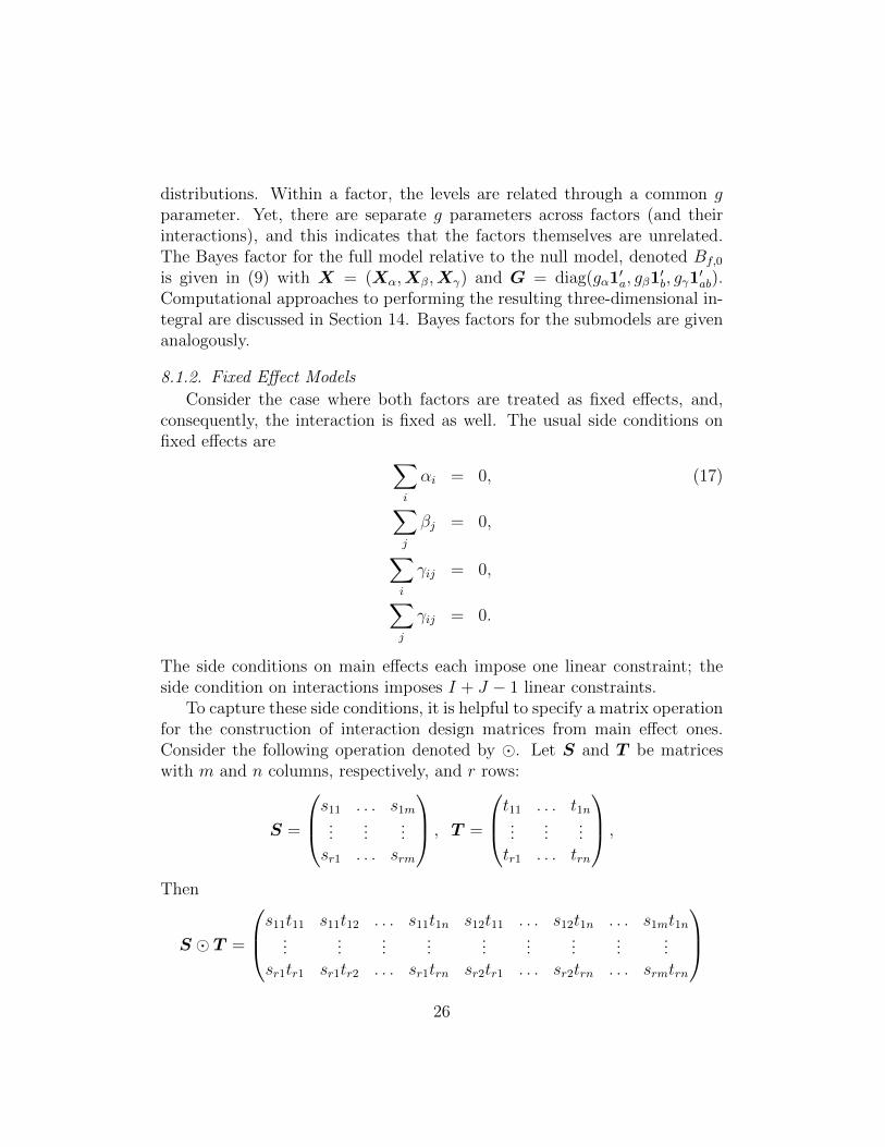
To capture these side conditions, it is helpful to specify a matrix operationfor the construction of interaction design matrices from main effect ones.Consider the following operation denoted by �. Let S and T be matriceswith m and n columns, respectively, and r rows:

S =

s11 . . . s1m...

......

sr1 . . . srm

, T =

t11 . . . t1n...

......

tr1 . . . trn

,

Then

S � T =

s11t11 s11t12 . . . s11t1n s12t11 . . . s12t1n . . . s1mt1n...

......

......

......

......

sr1tr1 sr1tr2 . . . sr1trn sr2tr1 . . . sr2trn . . . srmtrn

26

is a matrix of size r×mn. With this operation, design matrices of interactionsin factorial designs are given by

Xγ = Xα �Xβ.

The following full model captures the side conditions in (17):

y = µ1 + σ(X∗αα

∗ + X∗ββ∗ + X∗∗γ γ

∗∗)+ ε,

Main-effects parameter vectors α∗ and β∗ are of length a − 1 and b − 1,respectively, and the corresponding respective design matrices X∗α and X∗βare derived from the centering projection analogously to (13). The interactionparameter vector γ∗∗ is of length (a−1)(b−1), and the corresponding designmatrix is given by

X∗∗γ = X∗α �X∗β.

The use of two asterisks in the superscript on interaction parameters anddesign matrices indicates that there are separate sum-to-zero constraints onboth rows and columns in the matrix representation of interaction parame-ters. Prior specification of α∗, β∗, and γ∗∗ is analogous to (16). Moreover,all submodels are defined as the appropriate restriction on this full model.

8.1.3. Mixed Interactions

The development extends in a straightforward manner to mixed interac-tions. For example, suppose the first factor is fixed and the second is random.The model is given by

y = µ1 + σ(X∗αα

∗ + Xββ + X∗·γ γ∗·)+ ε.

where X∗·γ = X∗α �Xβ is a design matrix with (a − 1)b columns and γ∗· isan interaction vector of (a − 1)b effects which obeys the side constraint onrow sums of interactions but not on column sums. This parameterizationof mixed interactions is the same as in the classical Cornfield-Tukey mixedmodel (Cornfield & Tukey, 1956; Neter et al., 1996). Submodels are definedby various restrictions of this full model.

8.2. Assessment of Main Effects and Interactions

Conventional ANOVA is a top-down approach in which the total vari-ability is partitioned into main effects and interactions, and that which isresidual. Each main effect and interaction is separately assessed through a

27

comparison of the accounted variation relative to an appropriate error term.In the two-way case, researchers are interested in three comparisons: the twomain-effect comparisons and the interaction. Here, we recommend severaluseful Bayes factor model comparisons.

Assessing interactions is the most straightforward, and a top-down ap-proach that contrasts the performance of the full model to one without inter-actions is appropriate. We denote the corresponding Bayes factor by Bf,α+β.4

If the restriction without the target interaction is preferred to the full modelwith it, the interaction term is unnecessary to account for the data. Then,the appropriate Bayes factor to test the main effects of Factor 1 and Factor 2are Bf,β+γ and Bf,α+γ, respectively, and the effect in question is preferred ifthe full model has higher marginal likelihood than the restriction without it.In some contexts, the analyst may be interested whether there is any effectof a factor rather than just a main effect. In this case, corresponding Bayesfactor comparisons Bf,β and Bf,α are appropriate for assessing Factor 1 andFactor 2, respectively.

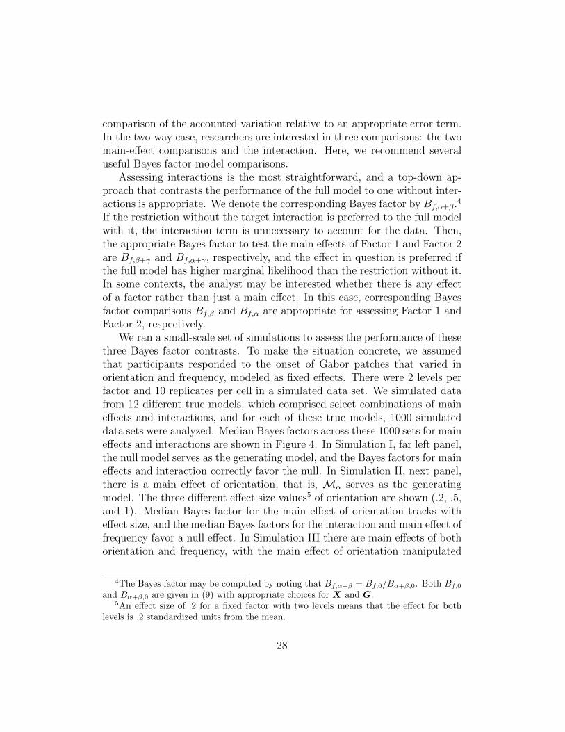
We ran a small-scale set of simulations to assess the performance of thesethree Bayes factor contrasts. To make the situation concrete, we assumedthat participants responded to the onset of Gabor patches that varied inorientation and frequency, modeled as fixed effects. There were 2 levels perfactor and 10 replicates per cell in a simulated data set. We simulated datafrom 12 different true models, which comprised select combinations of maineffects and interactions, and for each of these true models, 1000 simulateddata sets were analyzed. Median Bayes factors across these 1000 sets for maineffects and interactions are shown in Figure 4. In Simulation I, far left panel,the null model serves as the generating model, and the Bayes factors for maineffects and interaction correctly favor the null. In Simulation II, next panel,there is a main effect of orientation, that is, Mα serves as the generatingmodel. The three different effect size values5 of orientation are shown (.2, .5,and 1). Median Bayes factor for the main effect of orientation tracks witheffect size, and the median Bayes factors for the interaction and main effect offrequency favor a null effect. In Simulation III there are main effects of bothorientation and frequency, with the main effect of orientation manipulated

4The Bayes factor may be computed by noting that Bf,α+β = Bf,0/Bα+β,0. Both Bf,0and Bα+β,0 are given in (9) with appropriate choices for X and G.

5An effect size of .2 for a fixed factor with two levels means that the effect for bothlevels is .2 standardized units from the mean.

28

Med

ian

Bay

es F

acto

r F

or E

ffect

●●

●

●

●

●

●

●

●

●

● ●

M0 Mα

0.2 0.5 1Mα+β

0.2 0.5 1Mα+β

0.2 0.5 1

Mf

0.2 0.5

I. II. III. IV. V.0.

11

1010

00m

illio

n

● OrientationFrequencyInteraction

Figure 4: Median Bayes factor from simulated data. I. Data generated from the nullmodel. II. Data generated with main effects in orientation. True effect-size values fororientation were .2, .5, and 1. III. Same as previous simulation, except there was a truemain effect of frequency as well (true orientation effect-size values of .2, .5, and 1; truefrequency effect-size value of .4). IV. Data generated with equal-sized true main effectsin orientation and frequency. V. Data generated with main effects of both factors (trueeffect-size values of .4) and an interaction (true effect size values of .2 and .5). Orientationand frequency are modeled as fixed effects.

(.2, .5, 1) and the main effect of frequency held constant at .4. As can beseen, the Bayes factors track the true effect sizes well. Simulations IV andV show the case that there are two main effects of the same size, and whenthere are main effects and interactions, respectively. In all cases, the Bayesfactor performs as expected. One desirable property that is evident is anindependence or orthogonality. The Bayes factor for one comparison, say themain effect of orientation, does not depend on the true values of the otherfactors and interactions. This orthogonality mirrors that in conventionalANOVA analysis, and a necessary condition for it is separate g parametersacross main effects and interactions.

8.3. A Note on Fixed, Random, and Mixed Interactions

There is a trend in Bayesian analysis to treat effects as random in ANOVAdesigns. For one-way ANOVA, the Bayes factor for balanced designs is the

29

same whether the effects are modeled as fixed or random lending credence tothe notion that constraint from priors is in some abstract way comparableto explicitly imposing a sums-to-zero constraint. Unfortunately, this generalcomparability does not hold for interactions. Consider the 2×2 factorial casein which in the random-effects model there are 4 interaction effects, and theconstraint comes from the prior in which they are treated as exchangeable.Contrast this to the fixed-effect model where three sum-to-zero constraintsare imposed and there is subsequently one interaction parameter. We explorehow imposing the sum-to-zero constraints affects the Bayes factor throughevaluation of an example.

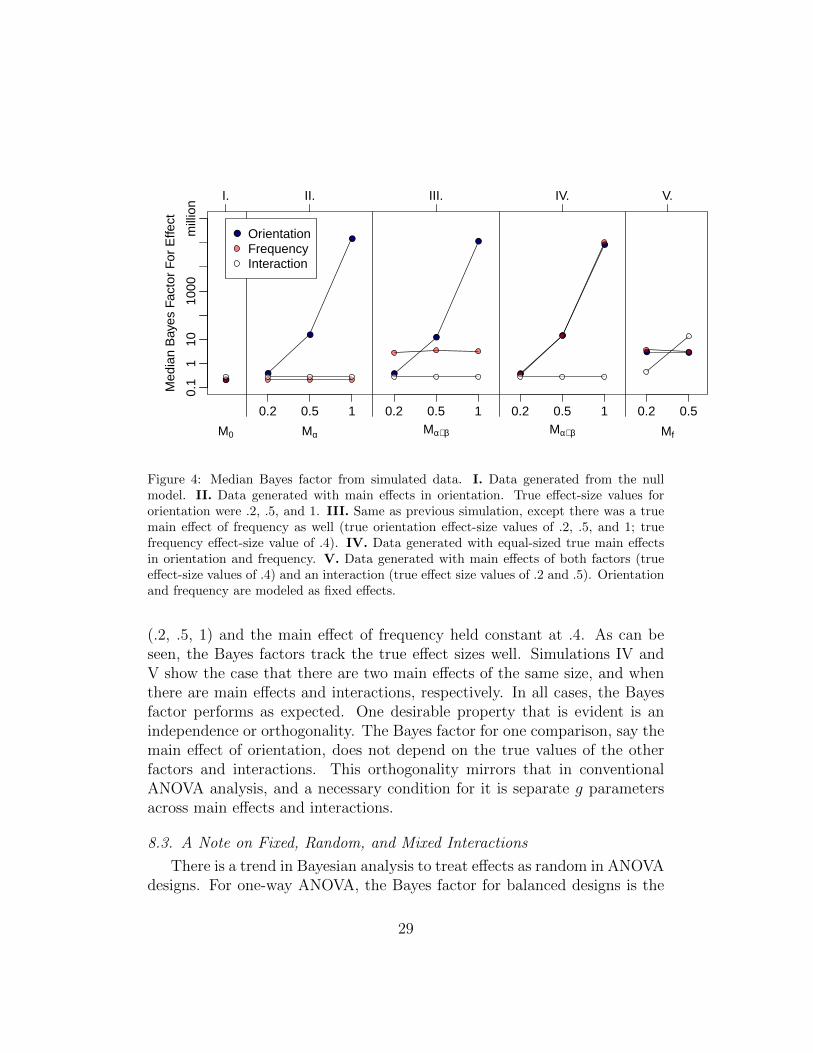
The table in Figure 5 shows hypothetical data from Model Mα in whichthere are only orientation effects. Classically, the F -value for orientationeffect in the fixed-effects model is obtained by dividing MSA by MSE, andit evaluates to F (1, 36) = 17.0, which, because the degrees-of-freedom in theerror term is high, results in a small p-value of .0002. For the random-effectsmodel, the F -value is obtained by dividing MSA be MSI , the interactionterm, and it evaluates to F (1, 1) = 28.3. Although this F -value is high, thecorresponding p-value is .12 because there is a single degree-of-freedom inthe error term. In classical statistics, evidence for an orientation effect inthis example is more easily detected when the effects are modeled as fixedrather than random. This makes sense: it should be easier to conclude thattwo levels differ than it is is to conclude that all possible levels differ whenthere are only two in a design.

Our default Bayes factors follow these classical patterns. Figure 5 showsthe resulting Bayes factors for the three contrasts and for four different typesof effects models. In the first model, darkest bars, the orientation and fre-quency are both considered fixed. In the second model, orientation is fixedand frequency is random, and their interaction is mixed with 2 parameters(dark grey bars). Included too is the complementary model (light grey bars)with random orientation and fixed frequency, and the random effects model(white bars), which has 4 interaction parameters. For all four models, thereis evidence for a null frequency effect and for a null interaction. These resultsare appropriate as the data were generated without these effects. There is adiscrepancy across the models in the assessment of the orientation main ef-fect. If frequency is considered fixed, the resulting Bayes factors yield strongevidence for an orientation effect; conversely, if frequency is considered ran-dom, the evidence is equivocal. Whereas the data are generated with a strongorientation effect, these random frequency models are hiding the underlying

30

Vertical HorizontalFreq. Low High Low High

0.7 0.53 0.87 0.970.71 0.52 0.72 0.90.68 0.82 0.85 0.670.57 0.78 0.82 0.660.6 0.6 0.81 0.60.68 0.67 0.88 0.610.57 0.76 0.84 1.070.67 0.65 0.94 0.890.62 0.49 0.94 0.710.75 0.63 0.68 0.6

Avg. .66 .65 .84 .77Orientation Frequency Interaction

Both FixedOrientation FixedFrequency FixedBoth Random

Bay

es F

acto

r vs

. Nul

l Mod

el

0.1

110

100

Figure 5: Left: Hypothetical response times (sec) to Gabor gratings that vary in orienta-tion (vertical vs. horizontal) and frequency (low vs. high) in a 2×2 design. Right: ResultingBayes factor for seven models when effects are modeled as fixed, mixed, or random.

structure. The reason they do so is that the random interactions are heavilyparameterized. It this case, this heavy parameterization leads to interactionsso flexible that they may account for main effect patterns.

This example highlights the usefulness of fixed-effects modeling. In manycases, random-effect models are inappropriate because they are too flexiblefor the experimental design and the questions of interest. Because of thisincreased flexibility, random and mixed interactions should be used withgreat care. Overall, we think the trend on Bayesian analysis to use randomeffects are a rule-of-thumb is unhelpful and analysts will gain be better servedby careful consideration of context in deciding between fixed and randomeffects. We think the prevailing rule-of-thumb that sum-to-zero constraintsshould be imposed for manipulated variables and not imposed for sampledlevels is a good one.

31

9. Within-Subject and Mixed Designs

The above development is appropriate to what are commonly referred toas between-subject designs, in which participants are nested within factors.Each participant performs under a single, specific combination of factors,and systematic variability across participants enters into the residual errorterms. In within-subject designs, in contrast, participants are crossed withthe levels of the factors, and each participant performs in all combinationsof the factors. It is reasonable to expect that participants vary substantially,and this variation induces a correlation in performance across conditions.A common approach is to include a separate factor for participant effects.Consider, for example, an experiment in which each participant identifiesGabor gratings at varying orientations. In the psychological literature, thisdesign is commonly referred to as a one-way within-subject design, where theone-way refers to the stimulus variable, orientation, and the within-subjectrefers to the fact that the levels are crossed with participants. Even thoughthis design is called one way, it is in fact a two-factor design with factorsfor participants and orientation. Likewise, what is commonly termed a two-way within-subject design has three factors: one participant factor and twostimulus factors.

The one-way within-subject design may be modeled with two-way ANOVAmodel. The following is appropriate when the stimulus variable is modeledas a fixed effect:

Mf : y = µ1 + σ(Xαα+ X∗ββ

∗ + X·∗γ γ·∗)+ ε. (18)

where α and β∗ are parameter vectors that describe the effect of partic-ipants and the levels of the stimulus factor, respectively. Included for fullgenerality is the mixed interaction term γ ·∗. This term may be estimated ifthe design is replicated, that is, each participant yields several observationsin each condition. In repeated measures designs, in which participants yielda single observation in each condition, it is not possible to distinguish theparticipants-by-treatment interaction term from the residual. In this case,the appropriate full model is Mα+β∗ .

Mixed designs occur when some factors are manipulated in a within par-ticipant manner and others are manipulated in a between participants man-ner. These designs may be treated analogously to within-subject designs. Inmixed designs, the design matrix on participant parameters codes which fac-

32

tors are manipulated in a within-subject manner and which are manipulatedin a between-subjects manner.

10. Theoretical Properties of Bayes Factors with Multiple g-parameterPriors

In Section 4.3, we listed three desirable properties of the one-sample Bayesfactor with a g-prior. These were scale invariance, consistency and consis-tency in information. Some of these properties are known to apply to theBayes factor in (9). Scale invariance, for example, is assured because thereis a scale-invariant prior on (µ, σ2), and the model is parameterized in termsof standardized effects rather than unstandardized effects.

Consistency is a more complicated concept in a factorial setting becausethere are multiple large-sample limits to be considered. Take the case ofthe two-factor design in which the sample size, N , is the product of threequantities: the number of levels of the first and second factors (a, b), andthe number of replicates in a cell r, N = abr. The sample size may in-crease to the limit by increasing any of these three quantities. Perhaps thesimplest case is when r, the number of replicates in a cell, is increased tothe limit while a and b are held constant. In this case, the model dimen-sionality is held constant as sample size increases. A more difficult case iswhen r is held constant and the number of levels of a factor is increase; i.e.,when say a is increased. In this case, increases in sample size correspondto an increase in model dimensionality. This second case is quite importantfor within-subject designs. In these designs, researchers increase sample sizeby adding additional subjects rather than by increasing the replicates persubject. Adding additional subjects entails adding more levels, that is, in-creasing model dimensionality. Hence, it is important to show consistency inthe large-model-dimension limit too.

Min (2011) studied the consistency properties of a more general class ofpriors in various large sample limits. He proved two facts of relevant here:First, if r is increased and the model dimensionality (a, b) is held constant,then Bayes factor (9) is consistent; that is, it approaches zero when the nullholds and ∞ when the specified model holds. Second, the Bayes factor isconsistent in the large a or large b limit when r is held constant. Therefore,researchers may use multiple g-priors in between-subject, within-subject, andmixed designs with assurance of correct limiting behavior.

33

To our knowledge, consistency in information, which refers to the correctlimit as the R2 approaches zero or 1, has not been studied in multiple g-parameter priors. It is known to hold for single-g parameter priors (Liang etal, 2008). Consistency in information is not as critical to us as consistencyin cell replicates or in model dimensionality, and the lack of theoretical workon this particular type of consistency should not dissuade adoption.

11. Inference With Multiple Random Effects: Memory and Lan-guage

Our development of default Bayes factors for ANOVA is exceedingly gen-eral. In this section, we illustrate the generality with an application to mem-ory and language studies. Inference is more complicated in memory andlanguage because in typical designs, researchers sample items from a cor-pus as well as people from a participant pool. The goal is to generalize theresults back to these corpra and populations. Consider a researcher whowishes to know if nouns are read at a different speed than verbs. Supposethe researcher samples 25 nouns and 25 verbs, and asks 50 participants toread each of these 50 words. In this case, there are three factors. The one ofsubstantive interest is the part-of-speech factor (noun vs. verb), which maybe modeled as a fixed effect. A second factor is an item factor. Individualnouns and verbs are assumed to have their own systematic effects above andbeyond their part-of-speech mean. The final factor is the effect of partici-pants, and each participant is assumed to have his or her own systematiceffect.

In many language studies, and in almost all memory studies, researchersaverage the results across items to construct participant-level scores. Theseparticipant-level scores are then submitted to a conventional ANOVA analy-sis. In the current example, a mean noun and verb reading time can be tab-ulated for each participant, and these scores may be submitted to a pairedt-test to assess the part-of-speech effect. This averaging approach, however,is known to be flawed because the Type I error rate will be inflated over nom-inal values. Clark (1973) noted that averaging treats items as fixed ratherthan as random effects, and the correlation in performance across items leadsto downward bias in the estimate of residual variability.

To demonstrate this downward bias, we performed a small simulation inwhich there is no true part-of-speech effect. Participants and items varied,and their individual effects are normally distributed with a standard devia-

34

●

●

●

●

●

●

●

●

●

p−va

lue

Item Aggregation

0.0

0.2

0.4

0.6

0.8

1.0

Bay

es fa

ctor

B01

0

2

4

6

8

10

12

Crossed Random Effects

Figure 6: Simulation of a word-naming experiment with systematic variation across par-ticipants and items. Data were generated from a null model in which there was no part-of-speech effect. The p-values are obtained from a t-test on participant-specific noun andverb means. The distribution of these p-values deviates substantially from a uniform, withan overrepresentation of small values. The Bayes factor are from the same data, but themodel includes crossed random effects of people and items. The Bayes factor favors theno part-of-speech effect null model.

tion of 100 ms. The residual error distribution has a standard deviation of150 ms. We performed 100 replicates in the simulation to explore the distri-bution of p-values, which is shown in the left box plot in Figure 6. If therewere no distortions due to averaging, then these p-values should be uniformlydistributed. The p-values deviate from a uniform distribution, and there isa dramatic over representation of small values. For a nominal .05 level, theobserved Type I error rate is .34.

Fortunately, researchers in linguistics are well aware of the problem ofinflated Type I error rates when items are aggregated. One recommendedsolution is to specify mixed linear models that treat people and items ascrossed random effects (Baayen et al., 2002). Mixed models may be analyzedin many popular packages including Proc Mixed in SAS, SPSS, and NMLE

35

in R. These more advanced models provide suitable Type I error control,that is, if there truly is no part-of-speech effect, the resulting p-values areuniformly distributed. Surprisingly, memory researchers have not adoptedcrossed random-effects modeling as readily as their linguistics colleagues (cf.,Pratte et al., 2010).

We show here Bayes factors for crossed-random effects may be conve-niently calculated. We implemented the following models to assess the part-of-speech effect for the above example in which 50 participants read 25 nounsand 25 verbs. In this case, there are a total of N = 50× 50 = 2500 observa-tions. Let X∗α be a 2500×1 design matrix that indicates whether the item isa noun or verb, and let Xλ and Xτ be 2500× 50 design matrices that mappeople and items into observations respectively. The full model is

M1 : y = µ1 + σ (X∗αα∗ + Xλλ+ Xττ ) + ε, (19)

where α∗ is a part-of-speech effect, and λ and τ are person and item randomeffects, respectively. The null model to assess part-of-speech effects is

M0 : y = µ1 + σ (Xλλ+ Xττ ) + ε. (20)

The Bayes factor for the two models is straightforwardly computed via (9),and the results are shown in the right box plot in Figure 6. The Bayes factorfor all 100 replicates of the experiment favor the null model between a factorof 6 to 12. This result is desirable as the data were simulated with no part-of-speech effect. Note here how researchers can state positive evidence for alack of an effect.

12. Alternative g-priors

In our development, we use separate g parameters for each factor. Thereare obvious alternatives. One is to use a single g parameter for all effectsregardless of factor; a second is to use a separate g-prior for each effect. Inthis section, we compare our choice to these alternatives.

12.1. A single g-prior

In the single-g prior, there is one g parameter for all main effects andinteractions, i.e, G = gI. Wetzels et al. (2012), for example, discuss thisapproach. Clearly, a single-g prior is more computationally efficient as theintegral in (9) is single-dimensional for all models. Nonetheless, we think

36

the single-g prior is inferior to the multiple-g prior for general use. Whenthere is one g, the pattern of effects on one factor calibrates the prior on theothers through the single g. For instance, take the case of two researcherswho wish to test the effect of part-of-speech (noun vs. verb) on word readingtimes. The first researcher uses one fixed effect, part-of-speech, and presentseach word for 300 ms. The second researcher crosses part-of-speech with asecond variable, presentation time, which is manipulated across two levels:299 ms and 301 ms. If these researchers use a single-g prior, the value ofg will be lower for the second researcher to reflect the assuredly null effectof presentation time. Hence, the Bayes factor for tests of part-of-speechwill differ, and, in particular, the second researcher will be more likely tointerpret small observed part-of-speech effects as evidence for a true effect.The multiple-g prior allows the inference about one factor to be independentof the patterns of effects in the other factors.

12.2. A separate g-parameter for each effect

Each element in the diagonal of G may be specified as a unique param-eter, and the marginal joint prior on effects is consequently the independentCauchy in (4). This prior, which is also a multiple g-parameter prior, haspotentially many more g parameters than the previous multiple g-parameterprior as there may be several levels for each factor. To differentiate thisprior from the previous one, we call this prior the independent Cauchy priorand reserve the term multiple g-parameter prior for the recommended onein which each factor rather than each effect is modeled with a separate gparameter.

We argue that the independent Cauchy prior is not ideal for ANOVA de-signs. Researchers use ANOVA specifically when effects can be decomposedinto factors. Factors, by their very nature, have a group structure that implya certain degree of coherence within a factor. For instance, consider the ori-entation and frequency factor in the previous example. The different levelsof orientation have a coherency in that they all describe a unified property;different levels of frequency also have a coherency. This coherence is cap-tured by the exchangeability of level (Gelman, 2005) as implemented by thecorrelations in the multivariate Cauchy. With this prior, effects of levels ofa factor cannot be arbitrarily different from one another.

There are some designs/models where the independent Cauchy prior ismore appropriate than the recommended multiple g-parameter prior, and

37

these designs do not have a factor structure. For example, consider the ques-tion of whether various diverse chemical compounds are agonists for a specificneural receptor. Without some knowledge of the structure of the compounds,there may be little coherency among them with regard to the ensuing recep-tor activity. In this case, the analyst is not interested in the mean effectof the compounds, or the variation around this mean. Instead, the analystassesses whether any specific compound serves as an agonist, and there isno hypothetical correlation or structure among the levels. The appropriatemodel is a cell-means model in which there is a separate standardized effectparameter for each cell, and an appropriate prior is the independent Cauchyprior. The multiple g-parameter prior, in contrast, embeds possible struc-ture among factors and is more appropriate for ANOVA designs in which theanalyst is concerned about main effects and interactions.

13. A Comparison To Default Regression Priors

In modern statistics it is common to think of ANOVA and regression in aunified linear models framework. Yet, we think researchers should be mindfulof some differences when considering categorical and continuous covariates.In the previous development, we advocated priors that led to Bayes factorsthat were invariant to the location and scale of measurement of the dependentvariable. With continuous covariates, it is desirable to consider an additionaltheoretical property: the Bayes factor should be invariant to the location andscale of the independent variable. For example, consider a researcher wishesto study intelligence as a function of height, the Bayes factor should notdepend on whether height is measured in inches or centimeters (or, for thatmatter, light years or angstroms), The following Bayes factor, from Zellnerand Siow (1980), obeys this property.

Let the linear model in (6) hold with the condition that each column ofXsums to zero. This condition is not substantive and provides no constraint;it simply guarantees that µ may be interpreted as a grand mean. Zellnerand Siow placed the noninformative prior π(µ, σ2) = 1/σ2 and the followingprior on standardized slopes θ:

θ | g ∼ Normal(0, g(X ′X)−1), g ∼ Scaled Inverse-χ2(N),

where the scaled inverse-χ2 distribution has density

f(x;h) = r−2(2π)−1/2(x/h)−3/2e−h/(2x), (21)

38

where h is a scale parameter. It is helpful to rewrite this prior so that thescale factor of N is in the variance of θ rather than in g:

θ | g ∼ Normal(0, g(X ′X/N)−1), g ∼ Inverse-χ2. (22)

The difference between the Zellner and Siow prior and the ones we developfor ANOVA (Eq. 7) is the introduction of a new scaling matrix X ′X/Nas well as the use of a single g-parameter. Because X is set to be zero-centered, this scaling term can be thought of as the variance or noise powerof the covariates. The scaling term is a matrix and includes the covariancesbetween covariates, making it appropriate for nonorthogonal covariates. Ahelpful interpretation is that there is a g-prior on double standardized effects,where effects is standardized to both the variability in the dependent variableand covariates, and are, consequently, without units. This scaling byX ′X/Nis necessary for the resulting Bayes factor to be invariant to the scale of theindependent variable. With this scaling in the prior, Liang et al (2008) derivethe following expression for the resulting Bayes factor against the null model:

Bf0 =

∫ ∞0

(1 + g)(N−p−1)/2[1 + g

(1−R2

)]−(N−1)/2 √N/2

Γ(1/2)g−3/2e−n/(2g)dg.

(23)

The introduction of the scaling termX ′X/N strikes us as very reasonablefor regression applications with continuous covariates, but less so for ANOVAapplications with categorical covariates. Consider the basic random effectsmodel given in (10) with a design matrix given by

X =

1 01 00 10 1

.

To meet the requirement that each column sums to zero, we subtract aconstant 1/2 from each entry:

D =

1/2 −1/21/2 −1/2−1/2 1/2−1/2 1/2

.

39

The resulting scale term is

D′D/N =

(1/4 −1/4−1/4 1/4

),

which is singular and cannot be inverted in the usual sense. One alternativeis to take a generalized inverse, which is proposed by Bayarri & Donato-Garcia (2007). Even with the generalized inverse, we are unsure that thescale term is well calibrated for the ANOVA case. Consider a balancedone-way ANOVA with a levels and r replicates and design matrix X =Ia ⊗ 1r. Note that (X ′X/N)−1 = aIa. Here, the prior variance on theeffects is proportional to the number of levels, which is indeed an unsatisfyingspecification.6 Moreover, it has undesirable implications for consistency. TheZellner-Siow priors lead to consistent Bayes factors if model dimensionalityis held constant, but they do not lead to consistent Bayes factors if modeldimensionality increases with sample size (Berger, Gosh, Mukhopadhyay,2003; Lang et al., 2008). In the current example, consistency would fail asa increases and r is kept constant. Because a scales the prior variance, inthe limit, this variance would grow without bound. Consequently, the Bayesfactor would favor the null regardless of the data. This behavior contrastsunfavorably with the ANOVA priors in (7), which lead to consistent Bayesfactors even as model dimensionality is increased with sample size.

We recommend that researchers choose priors based on whether the co-variate is categorical or continuous. It is appropriate to use (7) for categoricalcovariates and (22) for continuous ones. Models with both types of covari-ates may necessitate prior (7) on the categorical effects and prior (22) on thecontinuous effects.

14. Computational Issues

The critical step in computing Bayes factor is integrating the likelihoodfunction with respect to the prior distribution on parameters. All of themodels discussed have parameters µ, and σ2, and the non-null models haveadditional parameters θ and g. Computation of Bayes factors, therefore,

6This dependence of prior variance on the number of levels holds even if one centersthe design matrix so that the columns are orthogonal to 1 and then takes the generalizedinverse.

40

requires evaluation of high-dimensional integrals. For the proposed models,it is possible to derive closed-form expressions for the integrals over µ, σ2,and θ, and impossible to do so for g. Although the closed-form integrationgreatly reduces the dimensionality of integration relative to the number ofparameters, the resulting integral in (9) is still potentially multidimensional.The evaluation of this integral is the topic of this section.

We evaluate the multidimensional integral in (9) with a straightforwardform of Monte-Carlo sampling. Note that the Bayes factor in (9) may beexpressed as an expected value:

B10 = Eg[S(g)],

where the expectation is with respect to the prior distributions on g1, . . . , gr.This expectation value may be approximated by

Eg[S(g)] =1

L

L∑`=1

S(g`),

where g` is an r-dimensional random vector sampled from the joint prior ong.

The efficiency of this method is a function of the concentration of S(g)relative to the prior on g. If S(g) has large values on just a small rangeof g relative to the prior, then it will take a great many samples of g toaccurately estimate the integral. Conversely, if S(g) is spread across a widerange, then Monte Carlo integration may converge quickly. Fortunately, forcommonly used designs in experimental psychology, S(g) is relatively diffuse,and Bayes factors in (9) may be evaluated quickly and accurately with MonteCarlo integration.

Figure 7A illustrates why simple Monte Carlo integration of g parametersmay be effective. Shown are posterior and prior distributions of g for a fixed-effects ANOVA model with two levels on a single factor. There are fourparameters for this model: µ, σ2, α (standardized effect), and g. The criticalquantity is S(g), and it is proportional to the ratio of posterior and priordensities. As can be seen, the posterior is not much more concentratedthan the prior, implying that S(g) is also fairly diffuse. Although the figuredemonstrates the diffuseness of the posterior for a single-g parameter prior,this diffuseness is general and applies to multiple g-parameter priors as well.Figure 7B illustrates that the closed-form integration of the other parameters

41

Parameter g

Den

sity

0.0

0.2

0.4

0.6

0.8

1.0

0.01 1 100 10000 1e+06

A.

Effect Size

Den

sity

−2 −1 0 1 2

01

23

4

B.

Figure 7: Concentration of posterior relative to the prior. A. The posterior for g is nottoo concentrated relative to its prior, and Monte Carlo integration is relatively efficient.B. The posterior for effect-size (α) is more concentrated relative to prior, indicating thatthe closed-form integration over effects and variance is very helpful. The figure shows thecase for a two-group design with 100 observations in each group. The model is a one-way,fixed effects model with four parameters: µ, σ2, α and g.

is necessary. Shown are the posterior and prior distributions of α, on whicha standard Cauchy prior is placed. The posterior is quite concentrated,especially relative to the prior, and this concentration will slow convergenceof most numerical methods. In fact, the analytic integration of µ, σ2, θ inthe Appendix is critical for the convenient evaluation of (9).

In several cases, such as one-way ANOVA, or certain regression models,there may be a single g parameter. In this case, the integration in (9) isover a single dimension. We have found that Gaussian quadrature (Presset al., 1992) provides for quick and accurate estimation of Bayes factors, andrecommend it for these cases. With large samples, researchers should becognizant of numerical precision issues, and may have to fine-tune defaultquadrature algorithms. We have yet to explore Gaussian quadrature inte-gration across multiple dimensions, but given the properties of S(g), it mayserve as a reasonable alternative to Monte Carlo integration in this context.

There are alternative approaches to evaluating (9) than Gaussian quan-

42

drature or simple Monte Carlo integration. In cases where model dimen-sionality is large, it may prove necessary to use other sampling approaches,such as importance sampling (Ross, 2002) or bridge sampling (Meng & Wong,1996). Another alternative is to use MCMC-based approaches, such as evalu-ating the Savage-Dickey density ratio or its generalizations (Dickey & Lientz,1970; Verdinelli & Wasserman, 1995; Chib, 1995; Morey et al., 2011) or trans-dimensional MCMC (Carlin & Chib, 1995; see Lodewyckx, Kim, Lee, Tuer-linckx, Kuppens, & Wagenmakers, 2011 for a review). One approach that wehave tried that does not seem to work as well as hoped is Laplace approxima-tion (Gelman et al., 2004); the accuracy of the approximation is poor in somecases because the tails on the posterior of g diminish very slowly. The currentapproach of Monte Carlo sampling directly from the priors seems more con-venient than MCMC approaches because the analyst need not worry aboutmixing in MCMC chains.

We have implemented Gaussian quadrature (for one g-parameter priors)and Monte-Carlo sampling (for multiple g-parameter priors) in the bayesfactorPCLpackage for the R statistical software package. The package is currently inbeta development and can be found athttps://r-forge.r-project.org/projects/bayesfactorpcl/.

15. Bayes Factor for a Nonlinear Application: Skill Acquisition

The current development is for linear ANOVA and regression models.Yet, many mathematical psychologists are interested in the analysis of non-linear models. The current development must be modified, in some cases sig-nificantly, to accommodate nonlinearity. There are two general approachesthat may prove useful: Laplace approximation and Savage-Dickey densityratio evaluation. The Laplace approximation is based on assuming that theposterior can be well-approximated with a multivariate normal, which canbe integrated analytically. Sarbanes Bove & Held (2011) use the Laplaceapproximation to develop Bayes factors with g priors for the class of general-ized linear models (McCullagh & Nelder, 1989). Some psychological processmodels are members of the generalized linear model class, including Bradley-Terry-Luce scaling models (Bradley & Terry, 1952; Luce, 1959) and a wideclass of signal-detection models (DeCarlo, 1998). Several other psychologi-cal processing models fall outside the GLM class; examples include responsetime models with shift parameters that denote the lower bound of support,such as the TER shift parameter in Ratcliff’s (1978) diffusion model.

43

In this section we provide an example of a nonlinear application. Wedevelop a few nonlinear models, and compute the multiple-g prior Bayes fac-tor using the Savage-Dickey density estimation approach (Dickey & Lientz,1970; Morey et al., 2011). Our example is skill acquisition, and we addressthe particularly hard problem of assessing whether the speeding of the timeto complete a task falls as a power function or exponential function of theamount of practice. Prior to the work of Heathcote et al. (2000), it wasgenerally accepted that learning followed a power law with practice (e.g.,Newell & Rosenbloom, 1981), and this power law speed up was explained bya straightforward race-among-exemplars process (Logan, 1988, 1992). Es-timating learning curves has been a particularly vexing problem; althoughaveraging across participants seems attractive to reduce noise, the functionalform of the averaged data may not accurately reflect the functional form ofindividuals (Estes, 1956). Heathcote, Brown, and Mewhort (2000) providea particularly lucid description of the problem for assessing whether learn-ing is a power law or an exponential law. The power law describes a moreshallow decrease in learning than the exponential. Averaging data is knownto artifactually shallow the form of learning. Heathcote et al. showed thatif all individuals followed an exponential decrease (a steep form of learning),then the averaged data would approximate a power law even though it wasnot characteristic of any one individual.

Figure 8 provides some perspective on the difficulties of adjudicating be-tween power and exponential laws of learning. The panel shows mean taskcompletion time as a function of practice. The left panel shows data whereall individuals follow an exponential law, but there is variation in scale andshift across individuals that shallow the aggregate curve. Here, best fittingpower law and exponential laws are quite similar, and any analysis of meandata would be inconclusive. The right panel shows data where all individ-uals follow a power law. Neither power-law nor exponential-law fits to thedata are perfect, and each misses in slight but systematic ways. Here we seethat it is quite difficult to adjudicate between the functional forms form theanalysis of mean data aggregated across individuals.

We develop Bayesian hierarchical nonlinear power-law and exponential-law models with multiple g-priors and use Savage-Dickey density ratio esti-mation to compute the Bayes factor between the two models. In the exper-imental setup, a set of a individuals each perform a task J times, and thedependent variable is the time taken to complete the task. Let tij denotethis time for the ith participant on the jth trial, i = 1, . . . , a, j = 1, . . . , J .

44

0 50 100 150 200

1.0

1.2

1.4

1.6

1.8

Practice (# trials)

Tim

e (s

econ

ds)

Exponential−Law FitPower−Law Fit

A. True Exponential Law

0 50 100 150 200

1.0

1.5

2.0

2.5

3.0

Practice (# trials)

Tim

e (s

econ

ds)

B. True Power Law

Figure 8: Mean task completion time as a function of practice for simulated data. Meansare averages over 30 participants. Solid and dashed lines show best lest-squares fit for threeparameter exponential and power laws, respectively. A. Each individual’s data follow anexponential law and were generated with Me in (26). B. Each individual’s data followeda power law and were generated with Mp in (27).

45

As people repeat the task, they learn how to do it faster, and their timesdecrease. We model skill acquisition as a three-parameter, shifted lognormal:

log(tij − ψi) = µ+ αi + βxj + εij, (24)

where ψi serves an individual-specific shift parameter, µ is a grand mean onthe log scale, αi is a subject effect, xj is a covariate related to the level ofpractice, and β is a slope. Noise terms are

εijiid∼ Normal(0, σ2).

The lognormal is a unimodal distribution with an elongated right tail anda relatively soft rise, and all three of these properties are characteristic ofresponse time distributions. Not surprisingly, it has been recommended asboth a descriptive model and process model of RT (e.g., Ulrich & Miller,1993).

The lognormal is a shift-scale-shape model; parameter ψ describes theshift, parameters µ, α, and β describe the scale; parameter σ2 describes theshape. If xj = j, then expected value of response time follows an exponentiallaw:

E(tij) = ψi +Ki exp(β × j),

where Ki = exp(µ + αi + σ2/2) serves as a constant. Alternatively, if xj =log(j), then response time follows a power law:

E(tij) = ψi +Ki × jβ.

The fact that the power and exponential laws correspond to differentcovariates is very useful. Before stating the models, we standardized thelinear covariates (xj = j) and logarithm covariates (xj = log(j)) so theyhave a mean of 0 and a variance of 1. For the linear covariates, let w =1, . . . , J denote the vector of covariates, and let w and sw be the mean and(population) standard deviation of w, respectively. The standardized linearcovariate, denoted cj, is cj = (wj− w)/sw. Likewise for logarithm covariates,let v = (log(1), . . . , log(J)), v, and sv be the vector of covariates, its mean,and its (population) standard deviation, respectively. The standardized logcovariate, denoted dj, dj = (vj − v)/sv. The following three submodels of(24) serve as a null model (no skill acquisition), an exponential-law model,

46

and a power-law model:

M0 log(tij − ψi) = µ+ σαi + εij, (25)

Me log(tij − ψi) = µ+ σ(αi + βcj) + εij, (26)

Mp log(tij − ψi) = µ+ σ(αi + βdj) + εij, (27)

where effects are standardized with respect to σ2 as in the previous develop-ment. Priors are needed for all parameters. As before, noninformative priorsare placed on common parameters:

π(ψ, µ, σ2) = 1/σ2,

where ψ = (ψ1, . . . , ψa). Separate g-parameter priors are placed on partici-pant and covariate slope:

α | g1 ∼ Normal(0, g1Ia),

β | g2 ∼ Normal(0, g2),

gkiid∼ Inverse-χ2(1), k = 1, 2.

The key objective is to compute a Bayes factor between the power and ex-ponential law: Bpe. This Bayes factor is given by Bpe = Bp0/Be0, where Bp0

is the Bayes factor betweenMp andM0 and Be0 is the Bayes factor betweenMe and M0. If the shift ψi is zero for all people, then these Bayes factorscould be calculated with (9) by placing linear models on log yij. Unfortu-nately, empirical distributions of response time robustly exhibit substantialshifts (Rouder, 2005). Therefore, we implement an alternative Savage-Dickeyapproach to calculate Bp0 and Be0 as follows.

Models Mp and M0 are nested and differ by only the inclusion of slopeβ. Dickey & Lientz (1970) noted that in some cases the Bayes factor canbe expressed in this case as a ratio of posterior and prior densities of theparameter of interest, which in this case is β. Because Dickey and Lientzattributed the idea to Savage, this ratio is often called the Savage-Dickeydensity ratio. The ratio, denoted here as D0p, is

D0p =p(β = 0 | y)

p(β = 0), (28)

where the numerator and denominator are the posterior and prior probabil-ities, respectively, that β = 0 under Model Mp. The Savage-Dickey ratio is

47

equal to the Bayes factor B0p under the following independence conditions:Let η denote all parameters that are in M0, and let π0 denote the priordensity on these parameters. Let πp be the priors of the same parametersunder Mp. Then, the independence condition is given by

πp(η | β = 0) = π0(η).

Fortunately, this condition is satisfied by the standardized effect models in(26) and (27), and, consequently, D0p = B0p. The evaluation of the denomi-nator, p(β = 0) is straightforward. The marginal prior on β is a Cauchy, andits density evaluated at β = 0 is 1/π (where π is the mathematical constant).The evaluation of p(β = 0 | y), the posterior evaluated at β = 0, is morecomplicated. Wagenmakers et al. (2010) and Wetzels et al. (2010), who firstrecommended computation of the Savage-Dickey ratio in psychology, usedthe posterior samples of β to estimate the density at β = 0 through eithersplines or through a normal approximation. Chen (1994) and Gelfand andSmith (1990) recommend an alternative called conditional marginal densityestimation (CMDE) in which the probability that β = 0 is computed on eachiteration of the chain and averaged. Morey, Rouder, Pratte, and Speckman(2011) discuss these methods at length and performed a set of simulationsto characterize their properties. In all cases, CMDE outperformed the otherdensity estimation methods and is implemented here.

For our case, it is relatively straightforward to set up an MCMC chainto estimate parameters and the posterior density p(β = 0 | y). Derivationof conditional posteriors is straightforward (see Rouder and Lu, 2005, for atutorial in such derivations). Parameters ψ may be efficiently sampled withMetropolis-Hastings steps; parameters µ, α, and β may be treated as onemultivariate block and have a joint conjugate prior; variance parameters σ2,g1 and g2 have conjugate priors. These conjugate priors are convenient asthe corresponding parameters may be sampled with Gibbs steps. The keystep is evaluating the conditional posterior density of β at the point β = 0,and since this conditional is a normal density, evaluation is computationallyconvenient.

Bayes factors were computed by Savage-Dickey density ratios for the twosample data sets in Figure 8. The data for Figure 8A was generated fromMe with sizable uncorrelated individual variation in ψ and α; the data inFigure 8B was generated fromMp, again with sizable uncorrelated individualvariation. The resulting Bayes factor for the data in Figure 8A was Bpe =

48

7.4×10−31, indicating strong evidence for the exponential law. This behavioris desirable as the true data were generated with the exponential-law model.Likewise, the resulting Bayes factor for the data in Figure 8B was Bpe =1.4×106, which is also desirable as the data were generated by the power-lawmodel. As can be seen, g-prior Bayes factor assessment of the functional formof the learning curve is possible and convenient, and it is more principled andmore powerful than assessment from averaged data. In general, we suspectthat both Savage-Dickey density ratios and Laplace approximations will beuseful for developing g-prior Bayes factors in other nonlinear settings.

16. Conclusions

One goal in the analysis of experimental data is the assessment of theoriesthat specify constraints among observables. In service of this goal, there is ageneral need to be able to state evidence for invariances as well as for effects.The Bayes factor provides an approach to measuring evidence from data forcompeting theoretical positions, including those that specify invariances. Inthis regard, it provides a principled approach to accumulating evidence fornull hypotheses, an advantage not shared with null hypothesis significancetesting.

One of the necessary conditions for increased adoption of Bayes factoris development of default priors with associated algorithms for Bayes factorcomputation. Our approach herein is an objective approach in which priorsare chosen based on desirable theoretical properties of the resulting Bayesfactor. The defaults we advocate, combinations of multivariate and inde-pendent Cauchy priors on effects, lead to well-behaved Bayes factors thatare invariant to changes in measurement scale. The resulting computation isconvenient, especially when the number of g-parameters is relatively small.We therefore propose the default Bayes factor as a replacement for null hy-pothesis significance testing in regression, ANOVA, and other linear models.

We conclude with a few caveats. The current class of default priors doesnot free the researcher from making important decisions in analysis. Someof these decisions, such as specifying whether model factors are to be treatedas fixed or random, or specifying which models are to be compared, are notunique to Bayesian statistics. Other decisions, such as those involving thechoice of priors, are more specialized. The most consequential of these priorspecifications is the prior on effect parameters, and we have recommendeda combination of multivariate and independent Cauchy priors as a default

49

position. This recommendation is not a hard and fast rule, and it may beadapted as needed to reflect context about parameter variation, or, perhaps,the goals of inference. For example, researchers who a priori believe thatsmall effects in a domain are substantially important and highly probablemay wish to use a less diffuse prior than the Cauchy, or, perhaps, a Cauchyof reduced scale.7

Finally, we cannot escape the observations that (a) testing is not themost appropriate analysis in many situations, and that (b) testing is per-formed far too frequently in psychology. In fact, we characterize the fieldas having a testing fetishism in which common-sense exploratory analysesare sometimes ignored in favor of ill-suited hypothesis tests. For example,researchers are quick to resort to ANOVA as the main tool of analysis, evenin cases where null hypotheses are implausible a priori (Cohen, 1994; Morey& Rouder, 2011). They routinely test all main effects and interactions, oftencomplete with post-hoc tests of which levels are significantly different. Wenote that structure in data is sometimes not elucidated adequately by assess-ment of effects in linear models, and that exploratory and graphical methodsoften offer a more suitable alternative (Gelman, 2005; Wilkinson & the TaskForce on Statistical Inference, 1999). Researchers using testing, includingBayes factors, should keep in mind that they are trying to divine structurefrom comparisons among a set of models that are highly simplified represen-tations of nature. The implicit justification for testing is that a comparisonamong simplified models still yields useful insights into the structure of thedata and the relative applicability of various theoretical positions. This jus-tification will not always be present, and when it is not, other methods ofanalysis are better suited. Although we hope that researchers adopt Bayesfactor for their testing, we would find it problematic if they substituted afetishism with p-values for one with Bayes factor. In summary, the followingcompact tag line, adopted from a current beer commercial8, seems highlyappropriate: “I don’t always test, but when I do, I prefer Bayes factors.”

7The development is generalized to a scaled Cauchy prior on standardized effects withscale

√h by placing a scaled inverse-χ2 prior on g with scale h (see Eq.21). The marginal

likelihood in (8) and Bayes factor in (9) correspond to the case that h = 1, but are easilygeneralized for a scaled inverse-χ2 prior on g.

8The commercial for Dos Equis brand beer ends with the tag line, “I don’t always drinkbeer, but when I do, I prefer Dos Equis.” See www.youtube.com/watch?v=8Bc0WjTT0Ps.

50

Appendix

Proof of (8): We have the model specification and priors on µ, θ and σ2:

f(y | θ, µ, σ2) =1

(2π)N/2(σ2)N/2exp

(− 1

2σ2(y − 1µ−Xθ)′(y − 1µ−Xθ)

),

π(µ, σ2) = 1/σ2

π(θ | σ2, g) =1

(2π)P/2(σ2)P/2|G|1/2exp

(− 1

2σ2θ′G−1θ

),

where 1′ = (1, . . . , 1) is a vector of length p.The required marginal likelihood, m, is

m =

∫g1

· · ·∫gr

f(y | g)π(g) dg1 · · · dgr,

where

f(y | g) =

∫σ2

∫µ

∫θ

f(y,θ, µ, σ2 | g) dθ dµ dσ2, (29)

withf(y,θ, µ, σ2 | g) = f(y | θ, µ, σ2)π(θ | σ2, g)π(µ, σ2). (30)

The proof follows by showing that f(y | g) = Tm(g), where Tm is defined in(8).

Combining terms,

f(y,θ, µ, σ2 | g) =1

(2π)(N+P )/2(σ2)(N+P )/2+1|G|1/2exp

(− Q

2σ2

), (31)

where

Q = (y − 1µ−Xθ)′(y − 1µ−Xθ) + θ′G−1θ.

Now let P0 = 1N

11′ and complete the square in µ to obtain

Q = (y − 1µ)′(y − 1µ) +N(µ− 1

N1′(y −Xθ))2 − 1

N(1′(y −Xθ))2 + θ′G−1θ

= (y − 1µ)′(I − P0)(y − 1µ) +N(µ− 1

N1′(y −Xθ))2 + θ′G−1θ.

51

Thus∫ ∞−∞

f(y,θ, µ, σ2 | g) dµ =1

(2π)(N+P−1)/2(σ2)(N+P−1)/2+1|G|1/2√N

exp(− Q2

2σ2

),

whereQ2 = (y − Xθ)′(y − Xθ) + θ′G−1θ,

with y = (I − P0)y and X = (I − P0)X. (We have used the fact that(I − P0) is a perpendicular projection.)

Next, let Vg = X ′X +G−1 so that

Q2 = y′y + (θ − V −1g X ′y)′Vg(θ − V −1g X ′y)− y′X ′V −1g X ′y.

We then have∫ ∞−∞

∫f(y,θ, µ, σ2 | g) dµ dθ =

1

(2π)(N−1)/2(σ2)(N−1)/2+1|G|1/2√N |Vg|1/2

exp(− 1

2σ2(y′y − y′X ′V −1g X ′y)

).

Finally, integrating out σ2 yields (8).

52

References

Aitkin, M. (1991). Posterior Bayes factors. Journal of the Royal StatisticalSociety. Series B (Methodological), 53 , pp. 111–142.

Baayen, R. H., Tweedie, F. J., & Schreuder, R. (2002). The subjects as asimple random effect fallacy: Subject variability and morphological familyeffects in the mental lexicon. Brain and Language, 81 , 55–65.

Bayarri, M. J., & Garcia-Donato, G. (2007). Extending conventional priorsfor testing general hypotheses in linear models. Biometrika, 94 , 135–152.

Bem, D. J. (2011). Feeling the future: Experimental evidence for anomalousretroactive influences on cognition and affect. Journal of Personality andSocial Psychology , 100 , 407–425.

Berger, J. O., & Berry, D. A. (1988). Statistical analysis and the illusion ofobjectivity. American Scientist , 76 , 159–165.

Berger, J. O., Ghosh, J. K., & Mukhopadhyay, N. (2003). Approximationsto the Bayes factor in model selection problems and consistency issues.Journal of Statistical Planning and Inference, 112 , 241–258.

Berger, J. O., & Sellke, T. (1987). Testing a point null hypothesis: The irrec-oncilability of p values and evidence. Journal of the American StatisticalAssociation, 82 , 112–122.

Bradley, R. A., & Terry, M. E. (1952). Rank analysis of incomplete blockdesigns, I. the method of paired comparisons. Biometrika, 39 , 324–355.

Campbell, D. T., & Stanley, J. (1963). Experimental and Quasi-ExperimentalDesigns for Research. Boston, MA: Houghton-Mifflin.

Carlin, B. P., & Chib, S. (1995). Bayesian model choice via Markov chainMonte Carlo methods. Journal of the Royal Statistical Society. Series B(Methodological), 57 , pp. 473–484.

Chen, M.-H. (1994). Importance-weighted marginal Bayesian posterior den-sity estimation. Journal of the American Statistical Association, 89 , 818–824.

53

Chib, S. (1995). Marginal likelihood from the Gibbs output. Journal of theAmerican Statistical Association, 90 , 1313–1321.

Clark, H. H. (1973). The language-as-fixed-effect fallacy: A critique of lan-guage statistics in psychological research. Journal of Verbal Learning andVerbal Behavior , 12 , 335–359.

Cohen, J. (1994). The earth is round (p < .05). American Psychologist , 49 ,997–1003.

Cornfield, J., & Tukey, J. W. (1956). Average values of mean squares infactorials. Annals of Mathematical Statistics , 4 , 907–949.

Cox, R. T. (1946). Probability, frequency and reasonable expectation. Amer-ican Journal of Physics , 14 , 1–13.

De Finetti, B. (1992). Probability, induction and statistics : the art of guess-ing . Wiley.

DeCarlo, L. M. (1998). Signal detection theory and generalized linear models.Psychological Methods , 3 , 186–205.

Dehaene, S., Naccache, L., Le Clech, G., Koechlin, E., Mueller, M., Dehaene-Lambertz, G., van de Moortele, P.-F., & Le Bihan, D. (1998). Imagingunconscious semantic priming. Nature, 395 , 597–600.

Dickey, J. M., & Lientz, B. P. (1970). The weighted likelihood ratio, sharphypotheses about chances, the order of a Markov chain. The Annals ofMathematical Statistics , 41 , pp. 214–226.

Edwards, W., Lindman, H., & Savage, L. J. (1963). Bayesian statisticalinference for psychological research. Psychological Review , 70 , 193–242.

Estes, W. K. (1956). The problem of inference from curves based on groupeddata. Psychological Bulletin, 53 , 134–140.

Eves, H. (1980). Elementary Matrix Theory . Boston, MA: Allyn & Bacon.

Fechner, G. T. (1966). Elements of psychophysics . New York: Holt, Rinehartand Winston.

54

Gallistel, C. R. (2009). The importance of proving the null. PsychologicalReview , 116 , 439–453.

Gelfand, A., & Smith, A. F. M. (1990). Sampling based approaches to calcu-lating marginal densities. Journal of the American Statistical Association,85 , 398–409.

Gelman, A. (2005). Analysis of variancewhy it is more important than ever.Annals of Statistics , 33 , 1–53.

Gelman, A., Carlin, J. B., Stern, H. S., & Rubin, D. B. (2004). Bayesiandata analysis (2nd edition). London: Chapman and Hall.

Gelman, A., & Shalizi, C. R. (in press). Philosophy and the practice ofBayesian statistics. British Journal of Mathematical and Statistical Psy-chology , .

Gilovich, T., Vallone, R., & Tversky, A. (1985). The hot hand in basketball:On the misperception of random sequences. Cognitive Psychology , 17 ,295–314.

Good, I. J. (1979). Studies in the History of Probability and Statistics.XXXVII A. M. Turing’s Statistical Work in World War II. Biometrika,66 , pp. 393–396.

Hacking, I. (1965). Logic of Statistical Inference. Cambridge, England: Cam-bridge University Press.

Heathcote, A., Brown, S., & Mewhort, D. J. K. (2000). The power law re-pealed: The case for an exponential law of practice. Psychonomic Bulletinand Review , 7 , 185–207.

Jaynes, E. (1986). Bayesian methods: General background. In J. Jus-tice (Ed.), Maximum-Entropy and Bayesian Methods in Applied Statistics .Cambridge: Cambridge University Press.

Jeffreys, H. (1961). Theory of Probability (3rd Edition). New York: OxfordUniversity Press.

Johnson, N. L., Kotz, S., & Balakrishnan, N. (1994). Continuous UnivariateDistributions. Volume 2 (Second Edition). New York: Wiley.

55

Kass, R. E. (1992). Bayes factors in practice. Journal of the Royal StatisticalSociety. Series D (The Statistician), 2 , 551–560.

Kotz, S., & Nadarajah, S. (2004). Multivariate t distributions and theirapplications . Cambridge: Cambridge University Press.

Kruschke, J. K. (2011). Bayesian assessment of null values via parameterestimation and model comparison. Perspectives on Psychological Science,6 , 299–312.

Lee, M., & Wagenmakers, E. J. (2005). Bayesian statistical inference inpsychology: Comment on Trafimow (2003). Psychological Review , 112 ,662–668.

Liang, F., Paulo, R., Molina, G., Clyde, M. A., & Berger, J. O. (2008). Mix-tures of g-priors for Bayesian variable selection. Journal of the AmericanStatistical Association, 103 , 410–423.

Lindley, D. V. (1957). A statistical paradox. Biometrika, 44 , 187–192.

Liu, C. C., & Aitkin, M. (2008). Bayes factors: Prior sensitivity and modelgeneralizability. Journal of Mathematical Psychology , 56 , 362–375.

Lodewyckx, T., Kim, W., Tuerlinckx, F., Kuppens, P., Lee, M. D., & Wa-genmakers, E.-J. (2011). A tutorial on bayes factor estimation with theproduct space method. Journal of Mathematical Psychology , 55 , 331–347.

Logan, G. D. (1988). Towards an instance theory of automization. Psycho-logical Review , 95 , 492–527.

Logan, G. D. (1992). Shapes of reaction time distributions and shapes oflearning curves: A test of the instance theory of automaticity. Journal ofExperimental Psychology: Learning, Memory, and Cognition, 18 , 883–914.

Luce, R. D. (1959). Individual Choice Behavior . New York: Wiley.

Masin, S. C., Zudini, V., & Antonelli, M. (2009). Early alternative derivationsof Fechner’s law. Journal of the History of the Behavioral Sciences , 45 ,56–65.

McCullagh, P., & Nelder, J. A. (1989). Generalized linear models (2nd ed.).London: Chapman & Hall.

56

Meng, X., & Wong, W. (1996). Simulating ratios of normalizing constants viaa simple identity: a theoretical exploration. Statistica Sinica, 6 , 831–860.

Min, X. (2011). Objective Bayesian inference for stress=strength models andBayesian ANOVA. University of Missouri, Department of Statistics.

Morey, R. D., Romeign, W.-J., & Rouder, J. N. (). The humble bayesian:model checking from a fully bayesian perspective.

Morey, R. D., & Rouder, J. N. (2011). Bayes factor approaches for testinginterval null hypotheses. Psychological Methods , 16 , 406–419.

Morey, R. D., Rouder, J. N., Pratte, M. S., & Speckman, P. L. (2011). UsingMCMC chain outputs to efficiently estimate Bayes factors. Journal ofMathematical Psychology , 55 , 368–378.

Mulder, J., Klugkist, I., van de Schoot, R., Meeus, W. H. J., & Hoijtink, H.(2009). Bayesian model selection of informative hypotheses for repeatedmeasurements. Journal of Mathematical Psychology , 54 .

Murphy, S. T., & Zajonc, R. B. (1993). Affect, cognition, and awareness: Af-fective priming with optimal and suboptimal stimulus exposures. Journalof Personality and Social Psychology , 64 , 723–739.

Myung, I.-J., & Pitt, M. A. (1997). Applying Occam’s razor in modelingcognition: A Bayesian approach. Psychonomic Bulletin and Review , 4 ,79–95.

Neter, J., Kutner, M. H., Wasserman, W., & Nachtschiem, C. J. (1996).Applied linear regression models . Chicago: McGraw-Hill/Irwin.

Newell, A., & Rosenbloom, P. S. (1981). Mechanisms of skill acquisition andthe law of practice. In J. R. Anderson (Ed.), Cognitive skills and theiracquisition. (pp. 1–55). Hillsdale, NJ: Erlbaum.

Pratte, M. S., & Rouder, J. N. (2011). Hierarchical single- and dual-processmodels of recognition memory. Journal of Mathematical Psychology , 55 ,36–46.

57

Pratte, M. S., Rouder, J. N., & Morey, R. D. (2010). Separating mnemonicprocess from participant and item effects in the assessment of ROC asym-metries. Journal of Experimental Psychology: Learning, Memory, andCognition, 36 , 224–232.

Press, W. H., Teukolsky, S. A., Vetterling, W. T., & Flannery, F. P. (1992).Numerical Recipes in C: The art of Scientific Computing.. (second editioned.). Cambridge, England: Cambridge University Press.

Raftery, A. E. (1995). Bayesian model selection in social research. SociologicalMethodology , 25 , 111–163.

Ratcliff, R. (1978). A theory of memory retrieval. Psychological Review , 85 ,59–108.

Ross, S. M. (2002). Simulation. (3rd ed.). London: Academic Press.

Rouder, J. N. (2005). Are unshifted distributional models appropriate forresponse time? Psychometrika, 70 , 377–381.

Rouder, J. N., & Lu, J. (2005). An introduction to Bayesian hierarchicalmodels with an application in the theory of signal detection. PsychonomicBulletin and Review , 12 , 573–604.

Rouder, J. N., & Morey, R. D. (2011). A Bayes factor meta-analysis of Bem’sESP claim. Psychonomic Bulletin & Review , 18 , 682–689.

Rouder, J. N., & Morey, R. D. (in press). Default bayes factors for modelselection in regression. Multivariate Behavioral Research, .

Rouder, J. N., Speckman, P. L., Sun, D., Morey, R. D., & Iverson, G. (2009).Bayesian t-tests for accepting and rejecting the null hypothesis. Psycho-nomic Bulletin and Review , 16 , 225–237.

Royall, R. (1997). Statistical Evidence: A Likelihood Paradigm. New York:CRC Press.

Sarbanes Bove, D., & Held, L. (2011). Hyper-g priors for generalized linearmodels. Bayesian Analysis , 6 , 1–24.

Sellke, T., Bayarri, M. J., & Berger, J. O. (2001). Calibration of p values fortesting precise null hypotheses. American Statistician, 55 , 62–71.

58

Shibley Hyde, J. (2005). The gender similarities hypothesis. American Psy-chologist , 60 , 581–592.

Sternberg, S. (1969). The discovery of prossesing stages: Extensions of Don-der’s method. In W. G. Kosner (Ed.), Attention and Performance II (pp.276–315). Amsterdam: North-Holland.

Ulrich, R., & Miller, J. O. (1993). Information processing models generatinglognormally distributed reaction times. Journal of Mathematical Psychol-ogy , 37 , 513–525.

Vanpaemel, W. (2010). Prior sensitivity in theory testing: An apologia forthe Bayes factor. Journal of Mathematical Psychology , 54 , 491–498.

Verdinelli, I., & Wasserman, L. (1995). Computing Bayes factors using ageneralization of the Savage-Dickey density ratio. Journal of the AmericanStatistical Association, 90 , 614–618.

Wagenmakers, E.-J. (2007). A practical solution to the pervasive problem ofp values. Psychonomic Bulletin and Review , 14 , 779–804.

Wagenmakers, E.-J., Lodewyckx, T., Kuriyal, H., & Grasman, R. (2010).Bayesian hypothesis testing for psychologists: A tutorial on the Savage-Dickey method. Cognitive Psychology , 60 , 158–189.

Wetzels, R., Grasman, R. P., & Wagenmakers, E.-J. (2010). An encompassingprior generalization of the Savage-Dickey density ratio. ComputationalStatistics and Data Analysis , 54 , 2094–2102.

Wetzels, R., Grasman, R. P., & Wagenmakers, E.-J. (2012). A defaultbayesian hypothesis test for anova designs. American Statistician, .

Wetzels, R., Matzke, D., Lee, M. D., Rouder, J. N., Iverson, G., & Wa-genmakers, E.-J. (2011). Statistical evidence in experimental psychology:An empirical comparison using 855 t tests. Perspectives on PsychologicalScience, 6 , 291–298.

Wilkinson, L., & the Task Force on Statistical Inference (1999). Statisticalmethods in psychology journals. American Psychologist , 54 , 594–604.

59

Yonelinas, A. P. (1999). The contribution of recollection and familiarity torecognition and source-memory judgments: A formal dual-process modeland an analysis of receiver operating characteristics. Journal of Experi-mental Psychology: Learning, Memory, and Cognition, 25 , 1415–1434.

Zellner, A., & Siow, A. (1980). Posterior odds ratios for selected regressionhypotheses. In J. M. Bernardo, M. H. DeGroot, D. V. Lindley, & A. F. M.Smith (Eds.), Bayesian Statistics: Proceedings of the First InternationalMeeting held in Valencia (Spain) (pp. 585–603). University of Valencia.

60