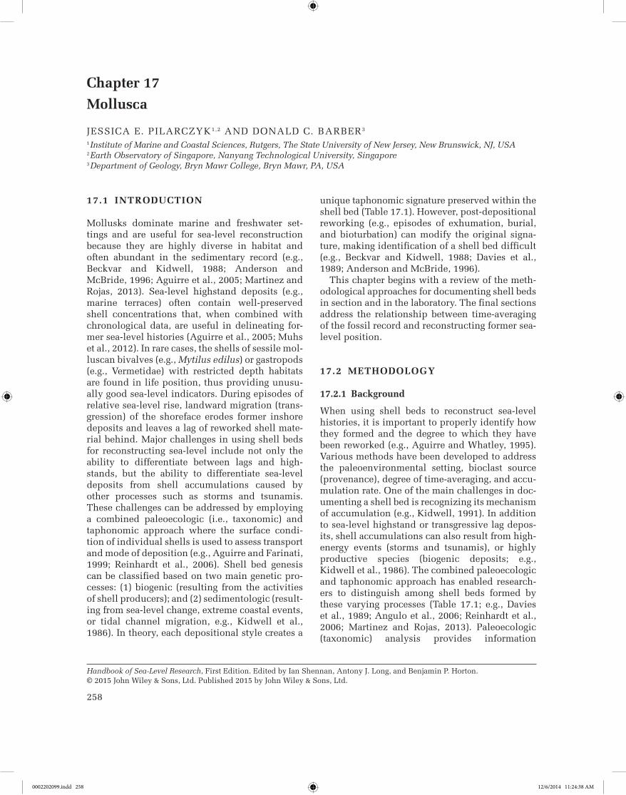
Handbook of Sea-Level Research, First Edition. Edited by Ian Shennan, Antony J. Long, and Benjamin P. Horton. © 2015 John Wiley & Sons, Ltd. Published 2015 by John Wiley & Sons, Ltd.

258

17.1 INTRODUCTION

Mollusks dominate marine and freshwater set-tings and are useful for sea-level reconstruction because they are highly diverse in habitat and often abundant in the sedimentary record (e.g., Beckvar and Kidwell, 1988; Anderson and McBride, 1996; Aguirre et al., 2005; Martinez and Rojas, 2013). Sea-level highstand deposits (e.g., marine terraces) often contain well-preserved shell concentrations that, when combined with chronological data, are useful in delineating for-mer sea-level histories (Aguirre et al., 2005; Muhs et al., 2012). In rare cases, the shells of sessile mol-luscan bivalves (e.g., Mytilus edilus) or gastropods (e.g., Vermetidae) with restricted depth habitats are found in life position, thus providing unusu-ally good sea-level indicators. During episodes of relative sea-level rise, landward migration (trans-gression) of the shoreface erodes former inshore deposits and leaves a lag of reworked shell mate-rial behind. Major challenges in using shell beds for reconstructing sea-level include not only the ability to differentiate between lags and high-stands, but the ability to differentiate sea-level deposits from shell accumulations caused by other processes such as storms and tsunamis. These challenges can be addressed by employing a combined paleoecologic (i.e., taxonomic) and taphonomic approach where the surface condi-tion of individual shells is used to assess transport and mode of deposition (e.g., Aguirre and Farinati, 1999; Reinhardt et al., 2006). Shell bed genesis can be classified based on two main genetic pro-cesses: (1) biogenic (resulting from the activities of shell producers); and (2) sedimentologic (result-ing from sea-level change, extreme coastal events, or tidal channel migration, e.g., Kidwell et al., 1986). In theory, each depositional style creates a

unique taphonomic signature preserved within the shell bed (Table 17.1). However, post-depositional reworking (e.g., episodes of exhumation, burial, and bioturbation) can modify the original signa-ture, making identification of a shell bed difficult (e.g., Beckvar and Kidwell, 1988; Davies et  al., 1989; Anderson and McBride, 1996).

This chapter begins with a review of the meth-odological approaches for documenting shell beds in section and in the laboratory. The final sections address the relationship between time-averaging of the fossil record and reconstructing former sea-level position.

17.2 METHODOLOGY

17.2.1 Background

When using shell beds to reconstruct sea-level histories, it is important to properly identify how they formed and the degree to which they have been reworked (e.g., Aguirre and Whatley, 1995). Various methods have been developed to address the paleoenvironmental setting, bioclast source (provenance), degree of time-averaging, and accu-mulation rate. One of the main challenges in doc-umenting a shell bed is recognizing its mechanism of accumulation (e.g., Kidwell, 1991). In addition to sea-level highstand or transgressive lag depos-its, shell accumulations can also result from high-energy events (storms and tsunamis), or highly productive species (biogenic deposits; e.g., Kidwell et al., 1986). The combined paleoecologic and taphonomic approach has enabled research-ers to distinguish among shell beds formed by these varying processes (Table  17.1; e.g., Davies et al., 1989; Angulo et al., 2006; Reinhardt et al., 2006; Martinez and Rojas, 2013). Paleoecologic (taxonomic) analysis provides information

Chapter 17

Mollusca

JESSICA E. PILARCZYK1,2 AnD DOnALD C. BARBER3

1 Institute of Marine and Coastal Sciences, Rutgers, The State University of New Jersey, New Brunswick, NJ, USA2 Earth Observatory of Singapore, Nanyang Technological University, Singapore3 Department of Geology, Bryn Mawr College, Bryn Mawr, PA, USA

0002202099.indd 258 12/6/2014 11:24:38 AM

Mollusca 259

concerning the depositional environment (e.g., autochthonous assemblage) and possible trans-port of mollusks (e.g., mixed assemblage), whereas taphonomic analysis provides further insight into the degree and type of transport and reworking (e.g., Davies et al., 1989; Aguirre et al., 2011).

Shell middens are subaerial cultural deposits comprised primarily of mollusk shells. In most cases, middens are readily distinguished from the types of shell beds considered in this chapter due to the morphology of the shell heaps, the tapho-nomic signatures resulting from selective harvest-ing, cooking, and consumption, and the presence of other cultural remains (Stein, 1992). The

allochthonous constituents of shell middens do not provide direct sea-level indicators, but the results of archeological studies on coastal shell middens are often integrated into regional sea-level reconstructions (e.g., Fairbridge, 1976; Angulo et al., 2006). In arid environments, defla-tion of eolian deposits containing numerous small shell middens can produce thin layers of mixed shells (Händel, 2009) that, upon initial examination, may resemble an event shell bed (e.g., storm overwash or tsunami deposit). Other archeological, sedimentologic, and geomorpho-logical evidence will generally reveal the cultural origin of reworked shell middens (Händel, 2009).

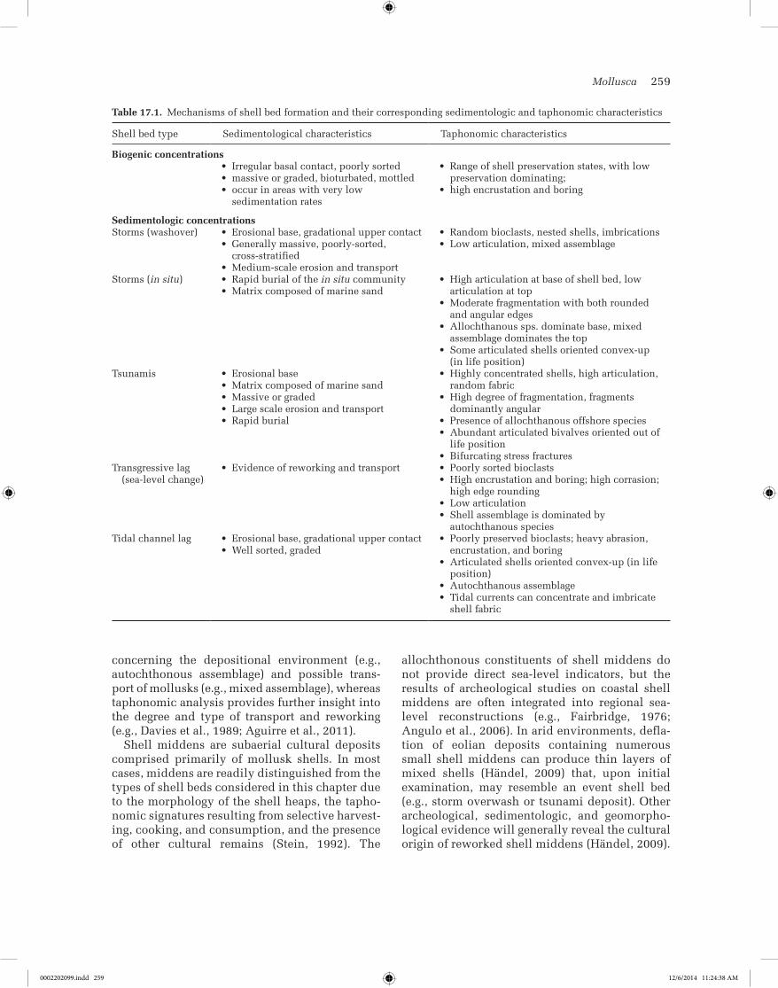
Table 17.1. Mechanisms of shell bed formation and their corresponding sedimentologic and taphonomic characteristics

Shell bed type Sedimentological characteristics Taphonomic characteristics

Biogenic concentrations•  Irregular basal contact, poorly sorted•  massive or graded, bioturbated, mottled•  occur in areas with very low

sedimentation rates

•  Range of shell preservation states, with low preservation dominating;

•  high encrustation and boring

Sedimentologic concentrationsStorms (washover) •  Erosional base, gradational upper contact

•  Generally massive, poorly-sorted, cross-stratified

•  Medium-scale erosion and transport

•  Random bioclasts, nested shells, imbrications•  Low articulation, mixed assemblage

Storms (in situ) •  Rapid burial of the in situ community•  Matrix composed of marine sand

•  High articulation at base of shell bed, low articulation at top

•  Moderate fragmentation with both rounded and angular edges

•  Allochthanous sps. dominate base, mixed assemblage dominates the top

•  Some articulated shells oriented convex-up (in life position)

Tsunamis •  Erosional base•  Matrix composed of marine sand•  Massive or graded•  Large scale erosion and transport•  Rapid burial

•  Highly concentrated shells, high articulation, random fabric

•  High degree of fragmentation, fragments dominantly angular

•  Presence of allochthanous offshore species•  Abundant articulated bivalves oriented out of

life position•  Bifurcating stress fractures

Transgressive lag (sea-level change)

•  Evidence of reworking and transport •  Poorly sorted bioclasts•  High encrustation and boring; high corrasion;

high edge rounding•  Low articulation•  Shell assemblage is dominated by

autochthanous speciesTidal channel lag •  Erosional base, gradational upper contact

•  Well sorted, graded•  Poorly preserved bioclasts; heavy abrasion,

encrustation, and boring•  Articulated shells oriented convex-up (in life

position)•  Autochthanous assemblage•  Tidal currents can concentrate and imbricate

shell fabric

0002202099.indd 259 12/6/2014 11:24:38 AM

260 Part 2: Laboratory Techniques

17.2.2 Field sampling

For locations where molluscan taxa and tapho-nomic trends are not well documented, a modern analog is useful in establishing taxonomic distribu-tions, which can then be applied down-core or in stratigraphic section to reconstruct the paleoenvi-ronment (e.g., Aguirre et al., 2011). This is accom-plished by determining relevant sub- environments for sampling, and then using a 30 cm × 30 cm metal frame to collect the upper 5 cm of sediment and shells (providing 4500 cm3 of sample material). Care must be taken to ensure that samples are not taphonomically overprinted through sampling (e.g., fragmentation and disarticulation).

The method for sampling shell beds in the field depends on the stratigraphic context, taxonomic group, age of the deposit, and shell size and con-centration (e.g., Reinhardt et al., 2006; Aguirre et  al., 2011). When examining shell deposits in the stratigraphic record, researchers can choose between core and trench sampling. Trenches or bank exposures are preferred because larger sam-ple sizes can be obtained, and they allow for the assessment of broadscale changes in contacts, grading, lithology, bioclasts, and bed geometry (e.g., Donato et al., 2008). Broad exposures are particularly useful for assessing shell orientation (e.g., in or out of life position), articulation of bivalves, imbrication, and nesting (stacking of shells inside one another). Further, larger species (e.g., Anadara sp., Tagelus sp.) will likely not be present in sufficient quantities in cores (e.g., Reinhardt et al., 2012). For bulk shell samples obtained from stratigraphic section, articulated specimens should be removed in the field to avoid disarticulation prior to analysis. Bulk samples can be stored below 5 °C in airtight plastic bags. Where coring is necessary, a minimum core diameter of 10 cm is recommended. Care must be taken to ensure that shell orientation is not affected during core recovery (Lanesky et al., 1979). Cores should be immediately sealed in plastic to prevent the sediment from drying or oxidizing and stored below 5 °C to prevent chemical and microbial alteration of the shell material. When document-ing shell beds the following should be noted (where possible) while in the field:

● stratigraphic context (e.g., surrounding units, bed geometry);

● lithology of the sediment matrix (e.g., clay, silt, sand, gravel);

● sedimentary structure (e.g., grading, bedding); ● contacts (e.g., erosional, gradational); ● concentration of shells (% volume of bioclasts; matrix- or bioclast-supported);

● lateral changes in species composition through-out the deposit;

● orientation of shells (e.g., random, imbricated, concave- or convex-up, and whether bivalves are in or out of life position);

● evidence of bioturbation; ● time-averaging (see Section 17.3).

17.2.3 Sample preparation

Sample preparation begins with washing bulk sam-ples over a 1 mm sieve using freshwater to remove sediment (e.g., De Francesco and Hassan, 2008). The main challenge in preparing shell samples for analysis is determining appropriate size classes. Highly fragmented samples, or those with a range of shell sizes, may benefit from multiple size classes (e.g., >2 mm fraction, <2 mm fraction). Fractioned samples can be placed in a drying oven at 25 °C overnight, or until dry. Mollusks are then sorted, identified to species level and counted. Following species identification, taphonomic characters are identified and counted, and the collective dataset is expressed as a percentage of overall mass or vol-ume. Depending on the study, considering a subset of target species within the assemblage may be more appropriate, particularly if the shell bed consists of a range of shell structures (e.g., thick, robust vs. thin, fragile). Some studies report varying tapho-nomic effects within the same deposit when using selected target species vs. bulk samples from the same stratigraphic unit (e.g., Aguirre et al., 2011). Aguirre et al. (2011) circumvented the bulk sam-pling bias in shell beds from Argentina by selecting two target species for taphonomic analysis.

17.2.4 Paleoecologic analysis (taxonomy and identification)

The Phylum Mollusca includes approximately 60,000 living species that span freshwater, brackish, and marine environments. Of all molluscan taxo-nomic classes, gastropods (e.g., snails) and bivalves (a shell with two hinged parts, e.g., clam) are gener-ally the most common components of shell beds (e.g., Davies et al., 1989; Anderson and McBride, 1996; Lopez et al., 2008). There is no universally accepted system for identifying mollusks, and iden-tification generally relies on anatomical features

0002202099.indd 260 12/6/2014 11:24:39 AM

Mollusca 261

such as shell shape and structure, foot, siphon, hinges, pallial line, and muscle scars (e.g., Mikkelsen and Bieler, 2007). Identification at higher taxonomic levels is complicated by morphological variation of these features and the loss of diagnostic soft parts. Although taxonomic effort is generally directed towards the mollusks in a shell deposit, noting the presence of other bioclasts (e.g., echinoids, bryozo-ans, barnacles, hydrozoans, algae) can be important in reconstructing depositional and paleoenviron-ment (estuarine vs. open marine conditions; e.g., Beckvar and Kidwell, 1988; Reinhardt et al., 2012).

17.2.5 Taphonomic analysis

Taphonomic alteration of a shell is a function of time and environmental conditions after death. Taphonomic analysis, involving the identification of taphonomic characters, enhances paleoenvi-ronmental interpretation (e.g., Davies et al., 1989; Kowalewski, 1996; Kidwell, 1998; Donato et al.,

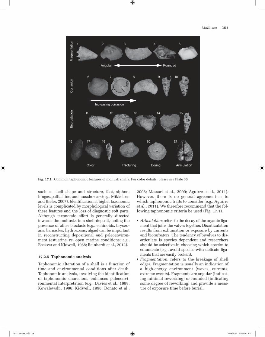
2008; Massari et al., 2009; Aguirre et al., 2011). However, there is no general agreement as to which taphonomic traits to consider (e.g., Aguirre et al., 2011). We therefore recommend that the fol-lowing taphonomic criteria be used (Fig. 17.1).

● Articulation: refers to the decay of the organic liga-ment that joins the valves together. Disarticulation results from exhumation or exposure by currents and bioturbators. The tendency of bivalves to dis-articulate is species dependent and researchers should be selective in choosing which species to enumerate (e.g., avoid species with delicate liga-ments that are easily broken).

● Fragmentation: refers to the breakage of shell edges. Fragmentation is usually an indication of a high-energy environment (waves, currents, extreme events). Fragments are angular (indicat-ing minimal reworking) or rounded (indicating some degree of reworking) and provide a meas-ure of exposure time before burial.

1

6

11

17

Color Fracturing Boring Articulation

18 19 20 2116

12 13 1514

Increasing corrasion

7 8 9 10

Angular

Frag

men

tatio

nC

orra

sion

Enc

rust

atio

n

Rounded

2 3 4 5

Fig. 17.1. Common taphonomic features of mollusk shells. For color details, please see Plate 30.

0002202099.indd 261 12/6/2014 11:24:40 AM

262 Part 2: Laboratory Techniques

● Corrasion: refers to the degradation of a shell caused by the combined effects of abrasion, dis-solution, and bioerosion (Brett and Baird, 1986). Mollusks that have undergone corrasion have chalky and pitted surfaces, loss of ornamenta-tion, and obscured features (e.g., loss of periostra-cum, indistinct pallial line, and muscle scars). Corrasion is related to subaerial exposure, energy of the environment, and size of the abrasive agent (e.g., Aguirre and Farinati, 1999), with sands and gravels being the most effective abrasives.

● Encrustation: refers to the attachment of other organisms onto a mollusk. Encrusters include sponges (Cliona), serpulid polychaetes, gastro-pods (e.g., Vermetidae), coral (Porites), red algae (Lithothamnion), barnacles, and bryozoans. The percentage of encrusted mollusks provides a measure of the duration of post-mortem expo-sure of shells on the sea floor, especially encrus-tation of infaunal shells which are out of reach of most encrusters while the organisms are alive in their burrows. Many encrusters are sensitive to even temporary burial by sediment.

● Color: refers to the degradation or bleaching of the original color due to exhumation, exposure, and aging.

● Fracturing: refers to the cracking or breaking of a shell. Bifurcating stress fractures are indica-tive of rapid shell fragmentation caused by tur-bulent-flow transport, shell-on-shell contact, and impact on hard surfaces such as rock or infrastructure (e.g., Donato et al., 2008).

● Orientation: refers to the position of a mollusk in stratigraphic section (random, imbricated, in life position, concave- or convex-up). High per-centages of articulated bivalves with random azimuthal orientation are often indicative of exhumation, transport, and rapid burial.

The collective consideration of paleoecologic and taphonomic data can be used to infer not only the origin of a shell bed, but also subsequent reworking or transport events. For example, a shell deposit consisting of both estuarine and marine species, where the estuarine species are less well-preserved than the marine species, indicates that the estuarine species are reworked and relict (e.g., Kidwell, 1998). However, a shell bed containing estuarine and marine species that are equally preserved indicates within-habitat time-averaging as opposed to environ-mental amalgamation (e.g., Kidwell, 1998). Furthermore, the combined approach enables the

differentiation between deposits generated by sea-level change and those created by storms or tsunamis (Table  17.1). For example, an assem-blage that consists of mollusks with low articula-tion but high abrasion and encrustation indicates that the shell material was exposed either con-tinuously or episodically after death. This is often seen in transgressive lag deposits (e.g., Anderson and McBride, 1996). On the contrary, storm deposits contain imbricated or nested shells with moderate fragmentation and minor articulation (Beckvar and Kidwell, 1988; Davies et al., 1989; Williams, 2011); whereas, tsunami shell beds contain high frequencies of shells that are articulated, fragmented, and contain bifurcat-ing stress fractures (Reinhardt et al., 2006; Donato et al., 2008).

17.2.6 Counting and data analysis

When quantifying the taxonomic and tapho-nomic composition of a shell deposit, a mini-mum of 300 specimens from each sample should be counted to fully capture the species/traits that are present, but in low abundance (e.g., Aguirre et al., 2011). In the case of bivalves, counts on disarticulated specimens can be divided by two to account for a whole specimen. The ultimate goal in data analysis is to ascribe a depositional origin. Multivariate techniques used to interpret these parameters include: ordi-nation methods (detrended correspondence analysis, non-metric multidimensional scaling), hierarchical clustering, and ternary diagrams (Kowalewski et al., 1995; Scarponi and Kowalewski, 2004; Hammer and Harper, 2006).

17.3 TIME-AVERAGING

A key problem when using molluscan assem-blages to reconstruct former sea-level is assessing the degree of time-averaging. Time-averaging is the process by which biological remains (e.g., mollusks) from different time intervals are accu-mulated together and preserved (Fürsich, 1990; Kidwell, 1998; Muhs et al., 2012). Over time, shell beds can be subjected to repeated cycles of physical reworking of host sediment (e.g., burial/exhumation) and bioturbation. Both of these pro-cesses result in time-averaging and a biasing of the geologic record over a broad range of time-scales (Kidwell, 1998). Determining the degree of

0002202099.indd 262 12/6/2014 11:24:40 AM

Mollusca 263

time-averaging is therefore important to interpret-ing the origin of a shell bed and placing it into proper chronological context.

Assessing the relative scale of time-averaging requires a combination of stratigraphic, sedimen-tologic, and paleontologic (taxa and taphonomy) evidence and is based on a four-step process of elimination (Kidwell, 1998). This process involves the categorization of shell accumula-tions into census, within-habitat time-averaged, environmentally condensed and biostratigraphi-cally condensed assemblages (Fig. 17.2; Kidwell and Bosence, 1991). Census assemblages are those that contain minimal time-averaging and record instantaneous or short-term events. Within-habitat time-averaged assemblages are character-ized by multiple generations of mollusks that are

from a single community, indicating environmen-tal stability. In contrast, environmentally con-densed assemblages contain ecologically unrelated species that accumulated over a period of environmental change. Assemblages that are time-averaged over longer timescales (>100 ka), and contain a mixture of species that span multi-ple chronozones, are referred to as biostratigraph-ically condensed.

Accumulation history is different from time-averaging because it refers to the time interval over which a shell bed forms. Accumulation his-tories range from instantaneous (e.g., storm, tsu-nami) to several thousands of years (e.g., sea-level change). Kidwell (1991) discusses the classifica-tion of four types of accumulation histories (from shortest to longest timescales): event; composite;

Step 1

Step 2

Step 3

Step 4

Censusassemblage?

assemblage?

Biostratigraphicallycondensed

assemblage?

Within-habitat time-averaged

assemblage?

Environmentally condensed

Type of time-averagedassemblage

Shells are taphonomically unalteredHigh articulationLife position is commonPreservation of soft tissues in some casesEvidence for rapid burial (e.g., graded bedding)

Taphonomic alteration?

No

No

No

Yes

Yes

Yes

Yes

Criteria

BeddingShells have distinctly different taphonomic characteristicsTaxa are discordant with matrixDiscontinuity (e.g., �ooding surface)

No bedding (homogenous matrix)Shells have one style of taphonomic alterationTaxa are in agreement with matrix

Mixture of species that span multiplechronostratigraphic ranges

Fig. 17.2. Identifying and interpreting the relative scale of time-averaging in shell beds using stratigraphic, sedimentologic, and paleontologic (taxa and taphonomy) evidence. Source: Kidwell, 1998. Reproduced with permission of Elsevier. The extremes, census, and biostratigraphically condensed assemblages are considered first in Steps 1 and 2, followed by the more common assemblage types (environmentally condensed and within-habitat time-averaged) in Steps 3 and 4.

0002202099.indd 263 12/6/2014 11:24:40 AM

264 Part 2: Laboratory Techniques

hiatal; and lag concentrations. Event concentra-tions (e.g., storm, tsunami) contain uniform pres-ervation and taxonomic composition. Composite concentrations, resulting from multiple events and slow sedimentation, contain variable taxa and preservation states. Hiatal concentrations form during prolonged intervals of sediment starvation, erosion, or reworking and are characterized by variable taxonomic composition and highly

variable preservation. Lag concentrations are shell beds that are produced by physical sorting and reworking of pre-existing beds. For example, transgressive lag concentrations contain predomi-nantly autochthonous taxa that are poorly pre-served (Fig. 17.3; Table 17.1). Lag concentrations generally have the lowest temporal resolution due to vigorous reworking (e.g., Anderson and McBride, 1996).

Eventconcentration

Hiatalconcentration

Lagconcentration

Preservation ofsingle events

Compositeconcentration

Average orexpanded section

Condensedsection

Amalgamation ofmultiple events

Brief episode of

shell accumulation

Removal of section byerosion/corrosion

Fig. 17.3. Mechanisms of shell bed formation (also known as accumulation history). Event concentrations, representing eco-logically brief episodes, can amalgamate as a result of physical and biological reworking. Amalgamated shell beds that are expanded are referred to as composite concentrations; those that are condensed are hiatal. A lag concentration forms when a portion of a shell bed is truncated by erosion/corrosion. Source: Adapted from Kidwell, 1991. Reproduced with permssion of Springer Verlag.

0002202099.indd 264 12/6/2014 11:24:40 AM

Mollusca 265

17.4 FOSSIL DATA AND SEA-LEVEL RECONSTRUCTIONS

For molluscan fauna to be used as a sea-level indicator they must possess a systematic and quan-tifiable relationship to elevation in the tidal frame (van de Plassche, 1986). Many sublittoral mollusks occupy a broad range of water depths (Petersen, 1986), so can only provide marine- limiting sea-level data points, with unconstrained one-way errors. nevertheless, in some cases, mollusk assem-blage data combined with sedimentologic, geomor-phologic and chronologic analyses, have helped to provide relatively narrow (2–5 m) paleo-sea-level ranges (e.g., Muhs et al., 2012).

Early studies employing mollusks as sea-level indicators were based on taxonomic analysis with little to no emphasis on taphonomy. Merrill et al. (1965) obtained radiocarbon dates from oyster beds (Crassostrea virginica) to construct a Holocene sea-level curve for the US Atlantic coast between Massachusetts and north Carolina. C. virginica was used as a qualitative reference to constrain former sea-level position due to its narrow range of habitat, restricted to shallow, brackish lagoons and estuaries. Over a decade later, MacIntyre et al. (1978) re-exam-ined the same oyster beds from north Carolina. High-resolution radiocarbon dates on individ-ual C. virginica shells indicated significant time-averaging and shoreward transport within the deposits. not only did these findings call into question previous sea-level reconstructions (e.g., Curray, 1965; Merrill et  al., 1965), they also highlighted the importance in understand-ing the degree of transport and time-averaging of an assemblage.

The addition of taphonomic analysis to tradi-tional paleoecological analysis on shell beds pro-vided better estimations of accumulation history and the degree of vertical mixing (e.g., Kowalewski, 1996; Kidwell, 1998). This combined approach has been used to assess former sea-levels from Europe (e.g., Gutierrez-Mas, 2011), South America (e.g., Aguirre and Whatley, 1995; Aguirre et al., 2005), and the Gulf of Mexico (e.g., Anderson and McBride, 1996). For example, extensive shell deposits in Argentina record a series of sea-level transgressions and regressions over the late Pliocene to late Quaternary (Aguirre and Whatley, 1995). These shell deposits are predominantly parautochthonous littoral ridges (e.g., beach ridges), but are also represented by tidal flat

deposits. Anderson and McBride (1996) showed that transgressive lag deposits, which are sub-jected to reworking and amalgamation as sea lev-els rise and fall, can still be recognized on the basis of their combined paleoecologic and tapho-nomic composition. Shelly transgressive lag deposits from the northeastern Gulf of Mexico are composed of well-preserved shells due to episodi-cally high sedimentation rates during high-energy events.

The use of mollusks in documenting former sea-levels is important deeper in the sedimentary record where post-depositional changes can entirely obscure thin sedimentary records. Episodes of sea-level transgression and regres-sion are archived in shell beds of late Pliocene age (e.g., Aguirre and Whatley, 1995). Older records have the added problem of decreasing preservation; time-averaging, hiatuses, and post-depositional alteration to shells can all lead to incomplete and misinterpreted records (e.g., Kidwell, 1998).

17.5 SUMMARY

Mollusks are useful indicators of sea level because they are abundant and readily recognizable in the stratigraphic record, and their habitat spans fresh-water to marine environments. Sea-level highstand and lag deposits form during cycles of sea-level transgression and regression and, when combined with chronological data, can be used to estimate former sea level. The resulting shell accumula-tions have unique taxonomic and taphonomic sig-natures that can be distinguished from one another. Through time, these shell beds can become over-printed by physical (e.g., storms, tides, waves) and biological (e.g., bioturbation) processes, thereby confounding the interpretation of past sea levels. Careful evaluation and determination of the type of shell bed under consideration, the characteris-tics of the bed, and its individual shell compo-nents provides a framework for using molluscan shell deposits for sea-level reconstruction. A com-bined taxonomic and taphonomic approach has been successfully used on shell accumulations to assess the origin (i.e., accumulation history), degree of time-averaging, and overall applicability of the deposit for sea-level studies. This technique has been used to reconstruct sea-level histories from several locations such as Europe, South America, and the Gulf of Mexico.

0002202099.indd 265 12/6/2014 11:24:40 AM

266 Part 2: Laboratory Techniques

ACKNOWLEDGEMENTS

This work was supported by the national Science Foundation (Award nos. EAR-1144537 and EAR-1322658).

REFERENCES

Aguirre, M.L., and Whatley, R.C. (1995) Late Quaternary marginal marine deposits and palaeoenvironments from northeastern Buenos Aires Province, Argentina: a review. Quaternary Science Reviews, 14, 223–254.

Aguirre, M.L., and Farinati, E.A. (1999) Taphonomic processes affecting late Quaternary molluscs along the  coastal area of Buenos Aires Province (Argentina, Southwestern Atlantic). Palaeogeography, Palae-oclimatology, Palaeoecology, 149, 283–304.

Aguirre, A., negro Sirch, Y., and Richiano, S. (2005) Late Quaternary molluscan assemblages from the coastal area of Bahía Bustamante (Patagonia, Argentina): paleo-ecology and paleoenvironments. Journal of South American Earth Sciences, 20, 13–32.

Aguirre, A., Richiano, S., Farinati, E., and Fucks, E. (2011) Taphonomic comparison between two bivalves (Mactra and Brachidontes) from Late Quaternary deposits in northern Argentina: which intrinsic and extrinsic fac-tors prevail under different palaeoenvironmental con-ditions? Quaternary International, 233, 113–129.

Anderson, L.C., and McBride, R.A. (1996) Taphonomic and palaeoenvironmental evidence of Holocene shell-bed genesis and history on the northeastern Gulf of Mexico shelf. Palaios, 11, 532–549.

Angulo, R.J., Lessa, G.C., and de Souza, M.C. (2006) A criti-cal review of mid- to late-Holocene sea-level fluctua-tions on the eastern Brazilian coastline. Quaternary Science Reviews, 25, 486–506.

Beckvar, n., and Kidwell, S.M. (1988) Hiatal shell concen-trations, sequence analysis, and sealevel history of a Pleistocene coastal alluvial fan, Punta Chueca, Sonora. Lethaia, 21, 257–270.

Brett, C.E., and Baird, G.C. (1986) Comparative taphonomy: a key to paleoenvironmental interpretation based on fossil preservation. Palaios, 1, 207–227.

Curray, J.R. (1965) Late Quaternary history, continental shelves of the United States. In The Quaternary of the United States (eds Wright, H.E., and Frey, D.C.), Princeton University Press, Princeton, nJ, 723–735.

Davies, D.J., Powell, E.n., and Stanton, R.J. (1989) Taphonomic signature as a function of environmental process: shells and shell beds in a hurricane-influenced inlet on the Texas coast. Palaeogeography, Palaeo-climatology, Palaeoecology, 72, 317–356.

De Francesco, C.G., and Hassan, G.S. (2008) Dominance of reworked fossil shells in modern estuarine environ-ments: implications for paleoenvironmental reconstruc-tions based on biological remains. Palaios, 23(1), 14–23.

Donato, S.V., Reinhardt, E.G., Boyce, J.I., Rothaus, R., and Vosmer, T. (2008) Identifying tsunami deposits using bivalve shell taphonomy. Geology, 36(3), 199–202.

Fairbridge, R.W. (1976) Shellfish-eating Preceramic Indians in Coastal Brazil. Science, 191, 353–359.

Fürsich, F.T. (1990) Fossil concentrations and life and death assemblages. In Palaeobiology (eds Briggs, D.E.G., and Crowther, P.R.), Blackwell Scientific Publications, London, p. 235–239.

Gutierrez-Mas, J.M. (2011) Glycymeris shell accumulations as indicators of recent sea-level changes and high-energy events in Cadiz Bay (SW Spain). Estuarine, Coastal and Shelf Science, 92, 546–554.

Hammer, O., and Harper, D. (2006) Paleontological Data Analysis. Blackwell Publishing, Oxford, 351 pp.

Händel, M. (2009) Al-Hamriya (Sharjah, UAE): approach-ing an extensive shell midden site. BioArchaeologica, 5, 103–112.

Kidwell, S.M. (1991) The stratigraphy of shell concentra-tions. In: Taphonomy: Releasing the Data Locked in the Fossil Record (eds Allison, P.A., and Briggs, D.E.G.), Plenum Press, new York, pp. 212–290.

Kidwell, S.M. (1998) Time-averaging in the marine fossil record: overview of strategies and uncertainties. Geobios, 30, 977–995.

Kidwell, S.M., and Bosence, D.W.J. (1991) Taphonomy and time-averaging of marine shelly faunas. In: Taphonomy: Releasing the Data Locked in the Fossil Record (eds Allison, P.A., and Briggs, D.E.G.), Plenum Press, new York, pp. 115–209.

Kidwell, S.M., Fürsich, F.T., and Aigner, T. (1986) Conceptual framework for the analysis and classifica-tion of fossil concentrations. Palaios, 1, 228–238.

Kowalewski, M. (1996) Time-averaging, overcompleteness, and the geologic record. Journal of Geology, 104, 317–326.

Kowalewski, M., Flessa, K.W., and Hallman, D.P. (1995) Ternary taphograms: triangular diagrams applied to taphonomic analysis. Palaios, 10, 478–483.

Lanesky, D.E., Logan, B.W., Brown, R.F., and Hine, A.C. (1979) A new approach to portable vibracoring under-water and on land. Journal of Sedimentary Petrology, 49, 654–657.

Lopez, R.A., Penchaszadeh, P.E., and Marcomini, S.C. (2008) Storm-related strandings of mollusks on the northeast coast of Buenos Aires, Argentina. Journal of Coastal Research, 24(4), 925–935.

MacIntyre, I.G., Pilkey, O.H., and Stuckenrath, R. (1978) Relict oysters on the United States Atlantic continental shelf: a reconsideration of their usefulness in under-standing late Quaternary sea-level history. Geological Society of America Bulletin, 89, 277–282.

Martinez, S., and Rojas, A. (2013) Relative sea level during the Holocene in Uruguay. Palaeogeography, Palaeo-climatology, Palaeoecology, 374, 123–131.

Massari, F., D’Alessandro, A., and Davaud, E. (2009) A coquinoid tsunamite from the Pliocene of Salento (SE Italy). Sedimentary Geology, 221(1–4), 7–18.

Merrill, A.S., Emery, K.O., and Rubin, M. (1965) Ancient oyster shells on the Atlantic continental shelf. Science, 147, 398–400.

Mikkelsen, P.M., and Bieler, R. (2007) Seashells of Southern Florida: Living Marine Mollusks of the Florida Keys and Adjacent Regions: Bivalves. Princeton University Press, Princeton, nJ.

Muhs, D.R., Simmons, K.R., Schumann, R.R., Groves, L.T., Mitrovica, J.X., and Laurel, D. (2012) Sea-level

0002202099.indd 266 12/6/2014 11:24:41 AM

Mollusca 267

history during the Last Interglacial complex on San nicolas Island, California: implications for glacial isostatic adjustment processes, paleozoogeography and tectonics. Quaternary Science Reviews, 37, 1–25.

Petersen, K.J. (1986) Marine molluscs as indicators of for-mer sea-level stands. In Sea-level Research: A Manual for the Collection and Evaluation of Data (ed. van de Plassche, O.), GeoBooks, norwich, pp. 129–155.

Reinhardt, E.G., Goodman, B.n., Boyce, J.I., Lopez, G., van Hengstum, P., Rink, W.J., Mart, Y. and Raban, A. (2006) The tsunami of December 13, 115 A.D., and the destruc-tion of Herod the Great’s harbour at Caesarea Maritima, Israel. Geology, 34, 1061–1064.

Reinhardt E.G., Pilarczyk, J.E., and Brown, A. (2012) Probable tsunami origin for a shell and sand sheet from

marine ponds on Anegada, British Virgin Islands. natural Hazards, 63, 101–117.

Scarponi, D., and Kowalewski, M. (2004) Stratigraphic paleoecology: bathymetric signatures and sequence overprint of mollusk associations from upper Quaternary sequences of the Po Plain, Italy. Geology, 32(11), 989–992.

Stein, J.K. (1992) Deciphering a Shell Midden. Academic Press, new York.

van de Plassche, O. (ed.) (1986) Sea-level Research: A Manual for the Collection and Evaluation of Data, GeoBooks, norwich.

Williams, H.L. (2011) Shell bed tempestites in the Chenier Plain of Louisiana: late Holocene example and a mod-ern analogue. Journal of Quaternary Science, 26(2), 199–206.

0002202099.indd 267 12/6/2014 11:24:41 AM