Chapter 13 - Student Solutions Manual Applied Statistics and Probability For
22
Chapter 13 - Student Solutions Manual Applied Statistics and Probability for Engineers, Fifth Edition https://www.safaribooksonline.com/library/view/student-solutions-manual/9780470888445/Chapter13.html[19/10/2015 23:36:36] CHAPTER 13 Section 13-2 13-1. a) Because factor df = total df – error df = 19 − 16 = 3 (and the degrees of freedom equals the number of levels minus one), 4 levels of the factor were used. b) Because the total df = 19, there were 20 trials in the experiment. Because there are 4 levels for the factor, there were 5 replicates of each level. c) From part (a), the factor df = 3 MS(Error) = 396.8/16 = 24.8, f = MS(Factor)/MS(Error) = 39.1/24.8 = 1.58. From Appendix Table VI, 0.1 < P-value < 0.25 d) We fail to reject H . There are not significance differences in the factor level means at α = 0.05. COTTON 4 475.76 118.94 14.76 0.000 Error 20 161.20 8.06 Total 24 636.96 Reject H and conclude that cotton percentage affects mean breaking strength. 0 0 PREV Chapter 12 NEXT Chapter 14 Student Solutions Manual Applied Statistics and Probability for Engineers, Fifth Edition Enjoy Safari? Subscribe Today
-
Upload
kingba-lawson-jack -
Category
Documents
-
view
268 -
download
19
Transcript of Chapter 13 - Student Solutions Manual Applied Statistics and Probability For
Chapter 13 - Student Solutions Manual Applied Statistics and Probability for Engineers, Fifth Edition
https://www.safaribooksonline.com/library/view/student-solutions-manual/9780470888445/Chapter13.html[19/10/2015 23:36:36]
CHAPTER 13
Section 13-2
13-1. a) Because factor df = total df – error df = 19 − 16 = 3 (and the degrees of
freedom equals the number of levels minus one), 4 levels of the factor were used.
b) Because the total df = 19, there were 20 trials in the experiment. Because there are
4 levels for the factor, there were 5 replicates of each level.
c) From part (a), the factor df = 3
MS(Error) = 396.8/16 = 24.8, f = MS(Factor)/MS(Error) = 39.1/24.8 = 1.58.
From Appendix Table VI, 0.1 < P-value < 0.25
d) We fail to reject H . There are not significance differences in the factor level
means at α = 0.05.
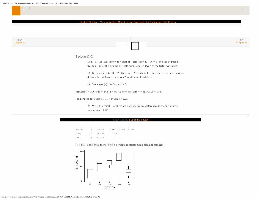
13-3. a) Analysis of Variance for STRENGTH
Source DF SS MS F P
COTTON 4 475.76 118.94 14.76 0.000
Error 20 161.20 8.06
Total 24 636.96
Reject H and conclude that cotton percentage affects mean breaking strength.
0
0
PREVChapter 12
NEXTChapter 14
Student Solutions Manual Applied Statistics and Probability for Engineers, Fifth Edition
Enjoy Safari? Subscribe Today
https://www.safaribooksonline.com/library/view/student-solutions-manual/9780470888445/Chapter12.html
https://www.safaribooksonline.com/library/view/student-solutions-manual/9780470888445/Chapter12.html
https://www.safaribooksonline.com/library/view/student-solutions-manual/9780470888445/Chapter12.html
https://www.safaribooksonline.com/library/view/student-solutions-manual/9780470888445/Chapter14.html
https://www.safaribooksonline.com/library/view/student-solutions-manual/9780470888445/Chapter14.html
Chapter 13 - Student Solutions Manual Applied Statistics and Probability for Engineers, Fifth Edition
https://www.safaribooksonline.com/library/view/student-solutions-manual/9780470888445/Chapter13.html[19/10/2015 23:36:36]
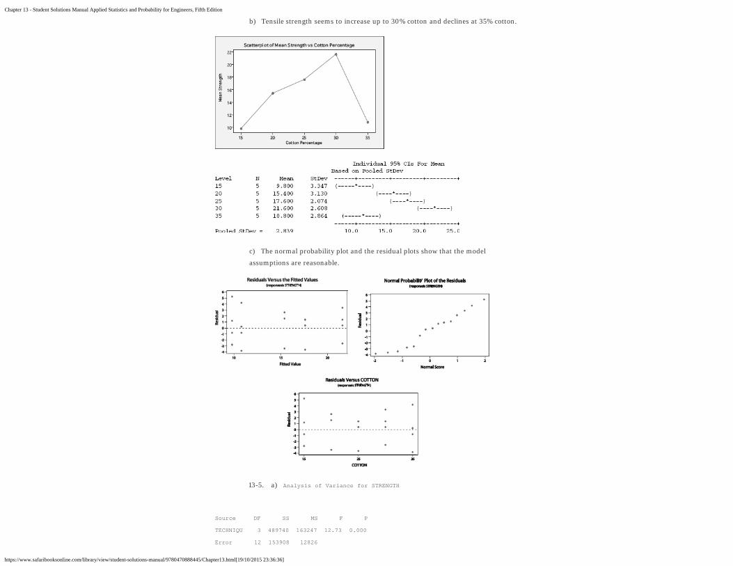
b) Tensile strength seems to increase up to 30% cotton and declines at 35% cotton.
c) The normal probability plot and the residual plots show that the model
assumptions are reasonable.
13-5. a) Analysis of Variance for STRENGTH
Source DF SS MS F P
TECHNIQU 3 489740 163247 12.73 0.000
Error 12 153908 12826
Chapter 13 - Student Solutions Manual Applied Statistics and Probability for Engineers, Fifth Edition
https://www.safaribooksonline.com/library/view/student-solutions-manual/9780470888445/Chapter13.html[19/10/2015 23:36:36]
Total 15 643648
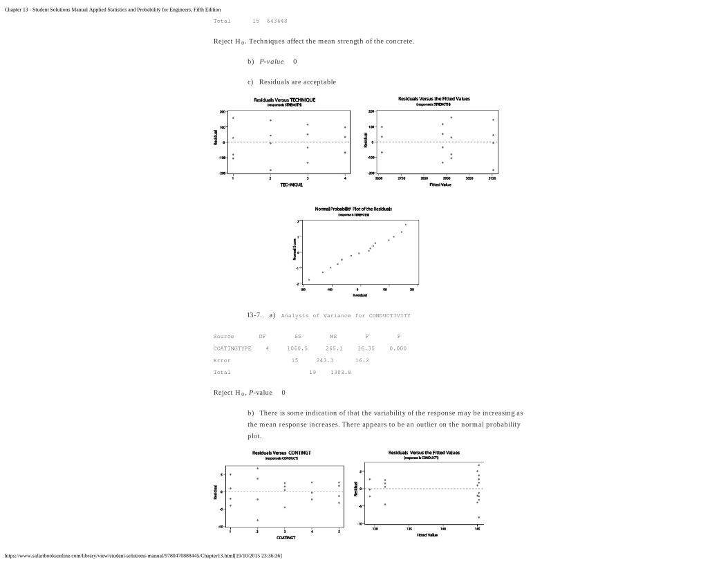
Reject H . Techniques affect the mean strength of the concrete.
b) P-value 0
c) Residuals are acceptable
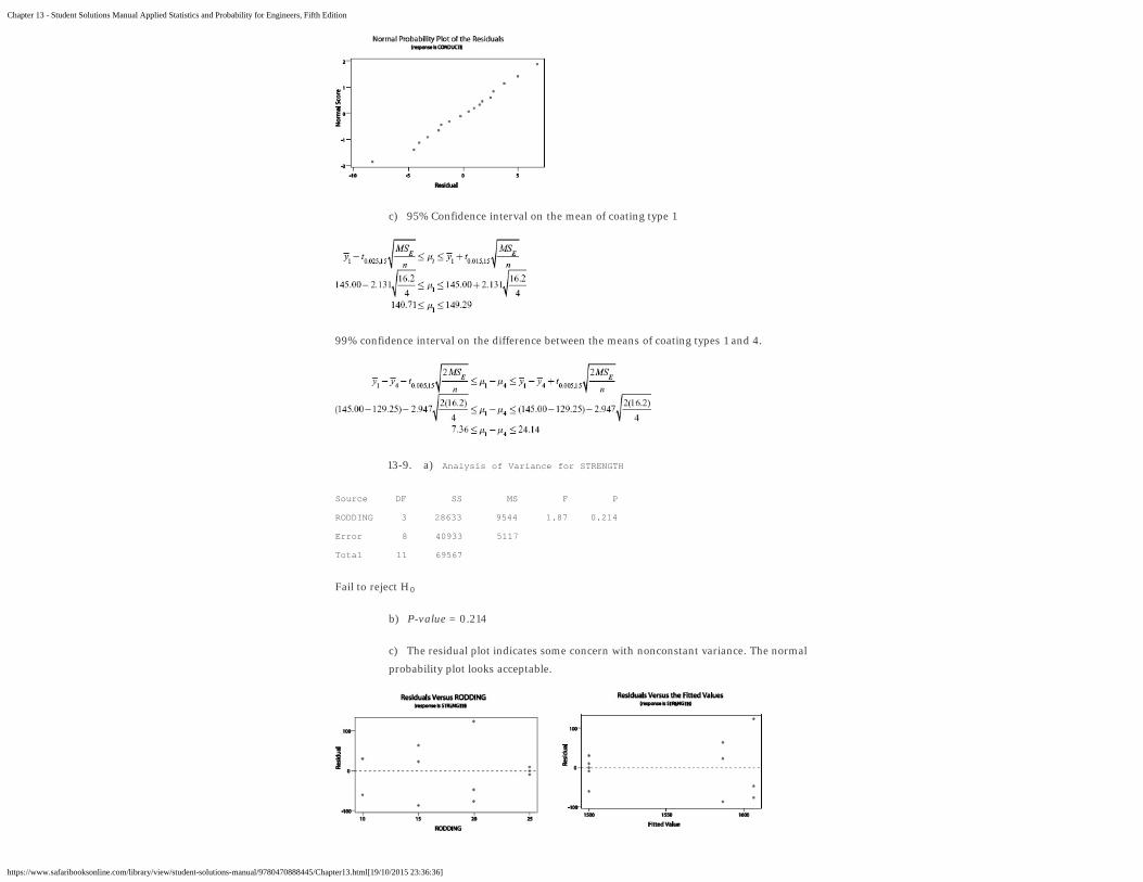
13-7. a) Analysis of Variance for CONDUCTIVITY
Source DF SS MS F P
COATINGTYPE 4 1060.5 265.1 16.35 0.000
Error 15 243.3 16.2
Total 19 1303.8
Reject H , P-value 0
b) There is some indication of that the variability of the response may be increasing as
the mean response increases. There appears to be an outlier on the normal probability
plot.
0
0
Chapter 13 - Student Solutions Manual Applied Statistics and Probability for Engineers, Fifth Edition
https://www.safaribooksonline.com/library/view/student-solutions-manual/9780470888445/Chapter13.html[19/10/2015 23:36:36]
c) 95% Confidence interval on the mean of coating type 1
99% confidence interval on the difference between the means of coating types 1 and 4.
13-9. a) Analysis of Variance for STRENGTH
Source DF SS MS F P
RODDING 3 28633 9544 1.87 0.214
Error 8 40933 5117
Total 11 69567
Fail to reject H
b) P-value = 0.214
c) The residual plot indicates some concern with nonconstant variance. The normal
probability plot looks acceptable.
0
Chapter 13 - Student Solutions Manual Applied Statistics and Probability for Engineers, Fifth Edition
https://www.safaribooksonline.com/library/view/student-solutions-manual/9780470888445/Chapter13.html[19/10/2015 23:36:36]
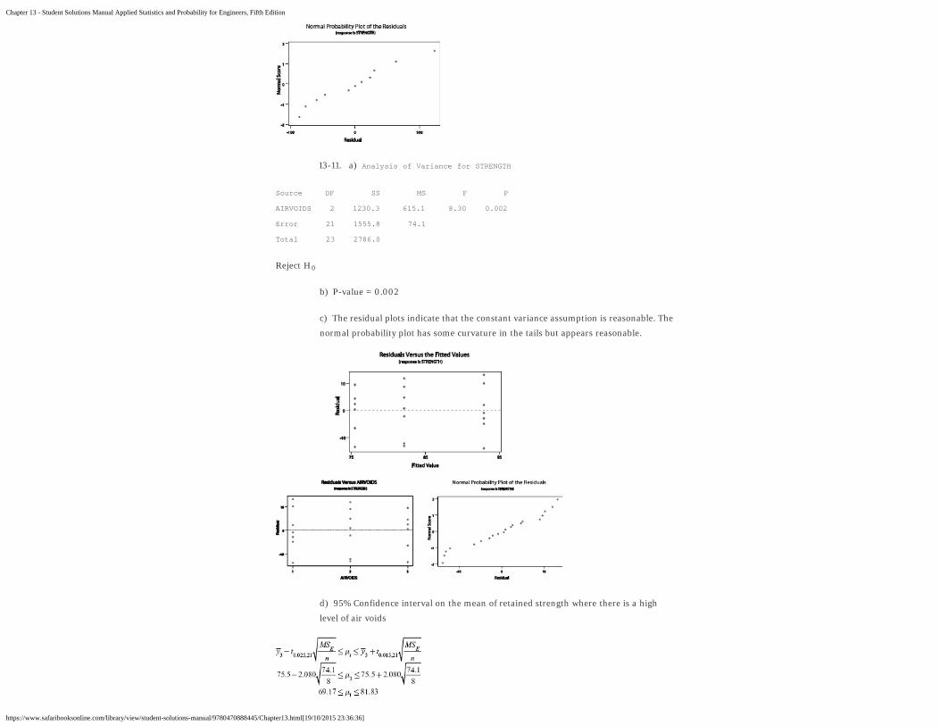
13-11. a) Analysis of Variance for STRENGTH
Source DF SS MS F P
AIRVOIDS 2 1230.3 615.1 8.30 0.002
Error 21 1555.8 74.1
Total 23 2786.0
Reject H
b) P-value = 0.002
c) The residual plots indicate that the constant variance assumption is reasonable. The
normal probability plot has some curvature in the tails but appears reasonable.
d) 95% Confidence interval on the mean of retained strength where there is a high
level of air voids
0
Chapter 13 - Student Solutions Manual Applied Statistics and Probability for Engineers, Fifth Edition
https://www.safaribooksonline.com/library/view/student-solutions-manual/9780470888445/Chapter13.html[19/10/2015 23:36:36]
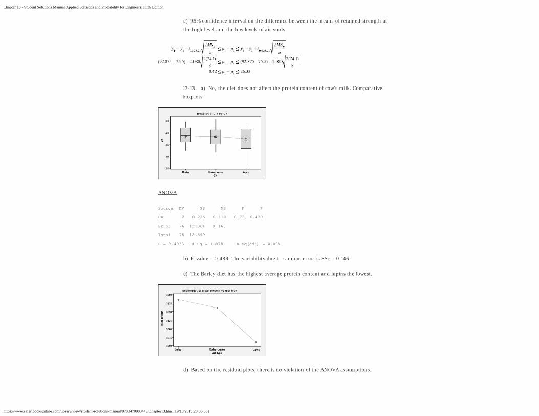
e) 95% confidence interval on the difference between the means of retained strength at
the high level and the low levels of air voids.
13-13. a) No, the diet does not affect the protein content of cow's milk. Comparative
boxplots
ANOVA
Source DF SS MS F P
C4 2 0.235 0.118 0.72 0.489
Error 76 12.364 0.163
Total 78 12.599
S = 0.4033 R–Sq = 1.87% R–Sq(adj) = 0.00%
b) P-value = 0.489. The variability due to random error is SS = 0.146.
c) The Barley diet has the highest average protein content and lupins the lowest.
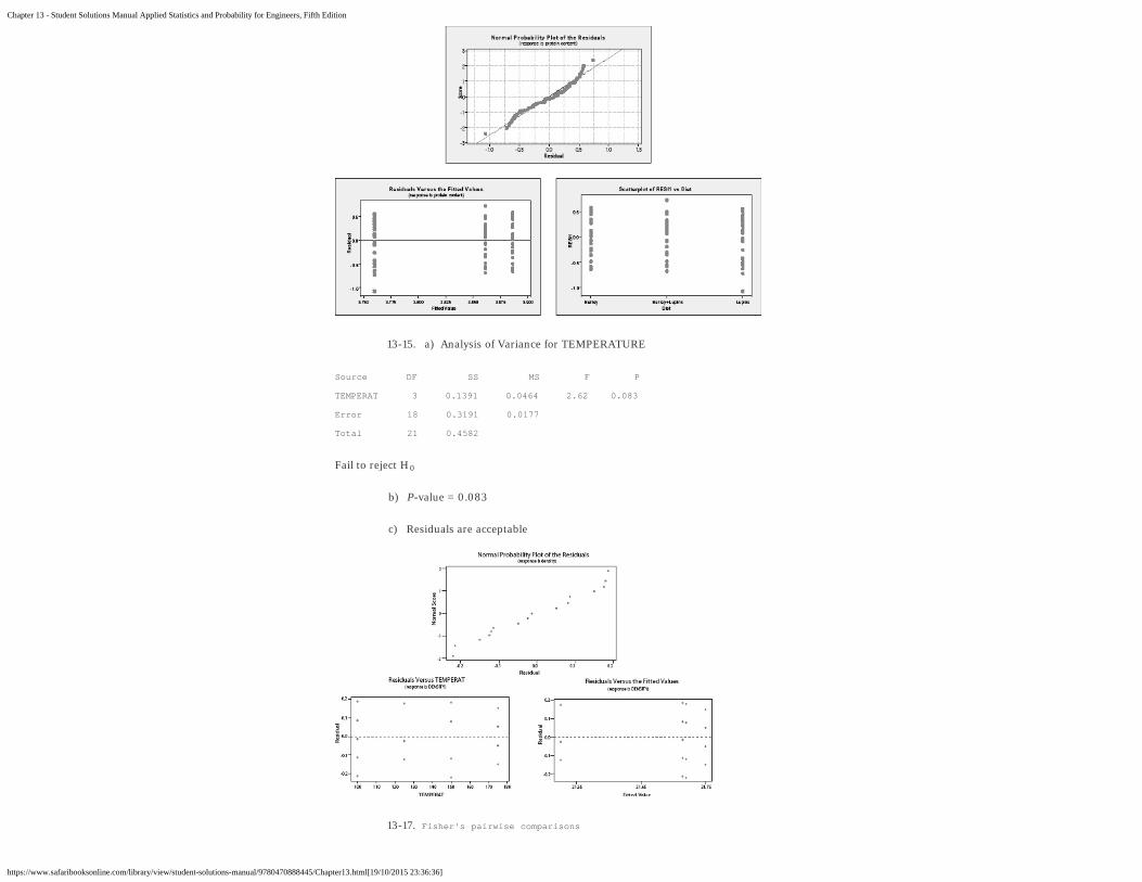
d) Based on the residual plots, there is no violation of the ANOVA assumptions.
E
Chapter 13 - Student Solutions Manual Applied Statistics and Probability for Engineers, Fifth Edition
https://www.safaribooksonline.com/library/view/student-solutions-manual/9780470888445/Chapter13.html[19/10/2015 23:36:36]
13-15. a) Analysis of Variance for TEMPERATURE
Source DF SS MS F P
TEMPERAT 3 0.1391 0.0464 2.62 0.083
Error 18 0.3191 0.0177
Total 21 0.4582
Fail to reject H
b) P-value = 0.083
c) Residuals are acceptable
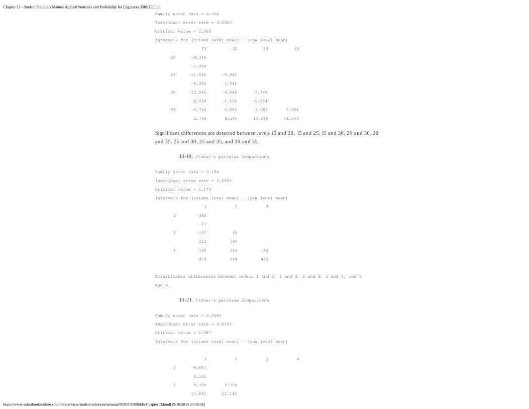
13-17. Fisher's pairwise comparisons
0
Chapter 13 - Student Solutions Manual Applied Statistics and Probability for Engineers, Fifth Edition
https://www.safaribooksonline.com/library/view/student-solutions-manual/9780470888445/Chapter13.html[19/10/2015 23:36:36]
Family error rate = 0.264
Individual error rate = 0.0500
Critical value = 2.086
Intervals for (column level mean) – (row level mean)
15 20 25 30
20 –9.346
–1.854
25 –11.546 –5.946
–4.054 1.546
30 –15.546 –9.946 –7.746
–8.054 –2.454 –0.254
35 –4.746 0.854 3.054 7.054
2.746 8.346 10.546 14.546
Significant differences are detected between levels 15 and 20, 15 and 25, 15 and 30, 20 and 30, 20
and 35, 25 and 30, 25 and 35, and 30 and 35.
13-19. Fisher's pairwise comparisons
Family error rate = 0.184
Individual error rate = 0.0500
Critical value = 2.179
Intervals for (column level mean) – (row level mean)
1 2 3
2 –360
–11
3 –137 48
212 397
4 130 316 93
479 664 442
Significance differences between levels 1 and 2, 1 and 4, 2 and 3, 2 and 4, and 3
and 4.
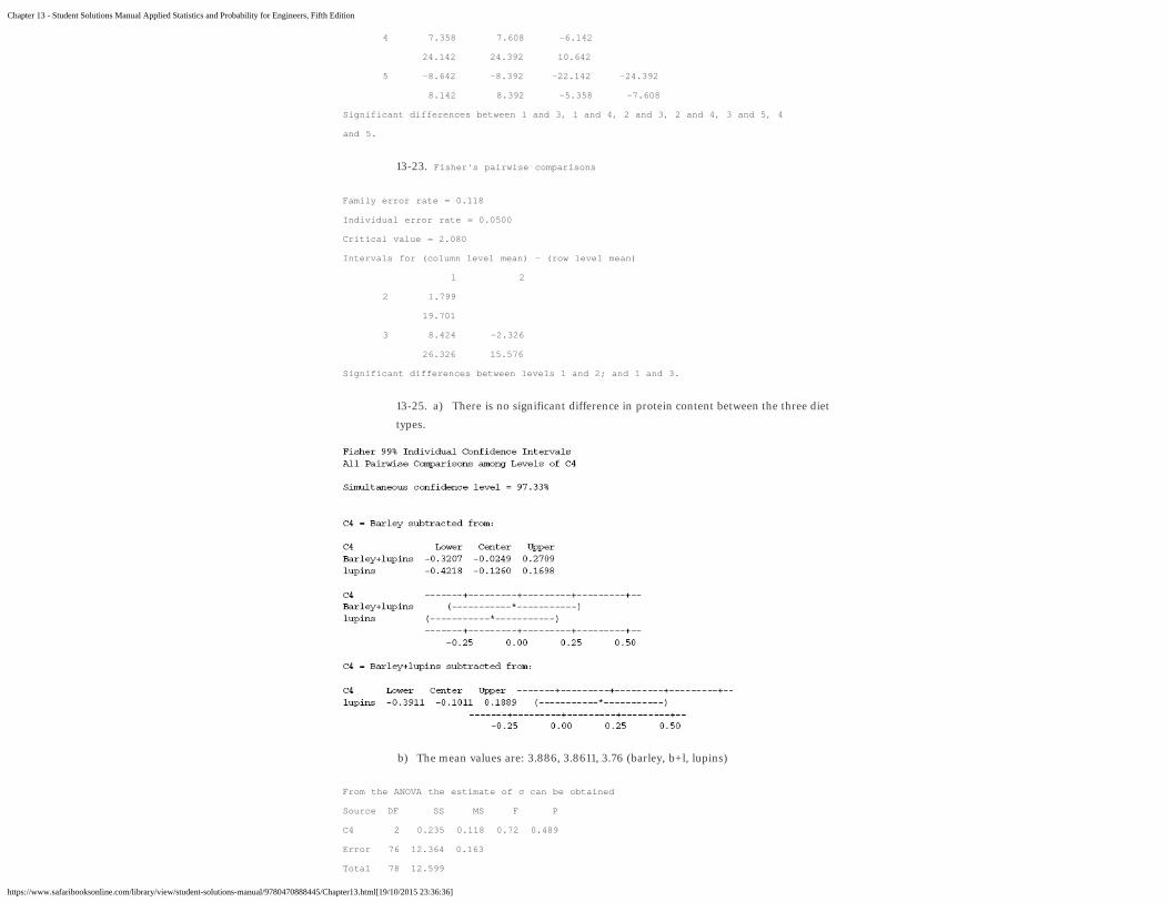
13-21. Fisher's pairwise comparisons
Family error rate = 0.0649
Individual error rate = 0.0100
Critical value = 2.947
Intervals for (column level mean) – (row level mean)
1 2 3 4
2 –8.642
8.142
3 5.108 5.358
21.892 22.142
Chapter 13 - Student Solutions Manual Applied Statistics and Probability for Engineers, Fifth Edition
https://www.safaribooksonline.com/library/view/student-solutions-manual/9780470888445/Chapter13.html[19/10/2015 23:36:36]
4 7.358 7.608 –6.142
24.142 24.392 10.642
5 –8.642 –8.392 –22.142 –24.392
8.142 8.392 –5.358 –7.608
Significant differences between 1 and 3, 1 and 4, 2 and 3, 2 and 4, 3 and 5, 4
and 5.
13-23. Fisher's pairwise comparisons
Family error rate = 0.118
Individual error rate = 0.0500
Critical value = 2.080
Intervals for (column level mean) – (row level mean)
1 2
2 1.799
19.701
3 8.424 –2.326
26.326 15.576
Significant differences between levels 1 and 2; and 1 and 3.
13-25. a) There is no significant difference in protein content between the three diet
types.
b) The mean values are: 3.886, 3.8611, 3.76 (barley, b+l, lupins)
From the ANOVA the estimate of σ can be obtained
Source DF SS MS F P
C4 2 0.235 0.118 0.72 0.489
Error 76 12.364 0.163
Total 78 12.599
Chapter 13 - Student Solutions Manual Applied Statistics and Probability for Engineers, Fifth Edition
https://www.safaribooksonline.com/library/view/student-solutions-manual/9780470888445/Chapter13.html[19/10/2015 23:36:36]
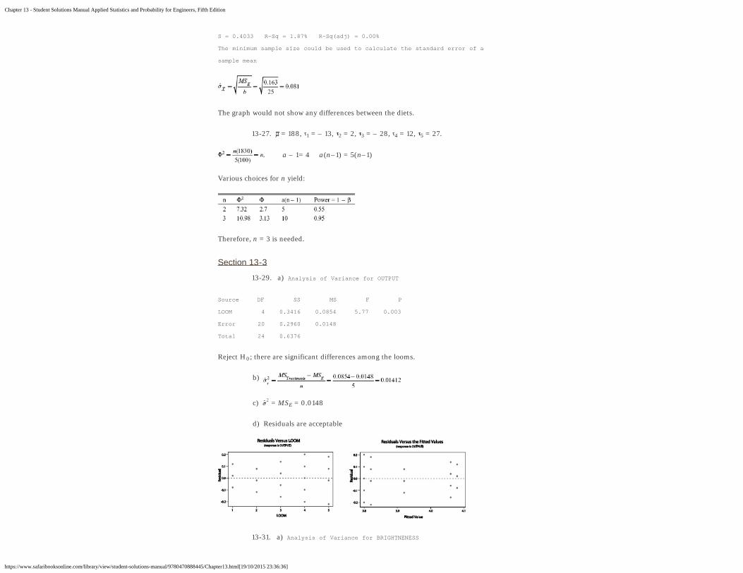
S = 0.4033 R–Sq = 1.87% R–Sq(adj) = 0.00%
The minimum sample size could be used to calculate the standard error of a
sample mean
The graph would not show any differences between the diets.
13-27. = 188, = – 13, = 2, = – 28, = 12, = 27.
a – 1= 4 a(n–1) = 5(n–1)
Various choices for n yield:
Therefore, n = 3 is needed.
Section 13-3
13-29. a) Analysis of Variance for OUTPUT
Source DF SS MS F P
LOOM 4 0.3416 0.0854 5.77 0.003
Error 20 0.2960 0.0148
Total 24 0.6376
Reject H ; there are significant differences among the looms.
b)
c) = MS = 0.0148
d) Residuals are acceptable
13-31. a) Analysis of Variance for BRIGHTNENESS
1 2 3 4 5
0
E2
Chapter 13 - Student Solutions Manual Applied Statistics and Probability for Engineers, Fifth Edition
https://www.safaribooksonline.com/library/view/student-solutions-manual/9780470888445/Chapter13.html[19/10/2015 23:36:36]
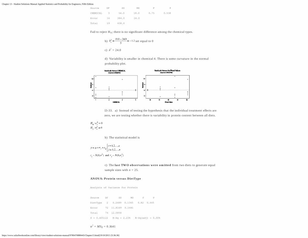
Source DF SS MS F P
CHEMICAL 3 54.0 18.0 0.75 0.538
Error 16 384.0 24.0
Total 19 438.0
Fail to reject H ; there is no significant difference among the chemical types.
b) set equal to 0
c) = 24.0
d) Variability is smaller in chemical 4. There is some curvature in the normal
probability plot.
13-33. a) Instead of testing the hypothesis that the individual treatment effects are
zero, we are testing whether there is variability in protein content between all diets.
b) The statistical model is
c) The last TWO observations were omitted from two diets to generate equal
sample sizes with n = 25.
ANOVA: Protein versus DietType
Analysis of Variance for Protein
Source DF SS MS F P
DietType 2 0.2689 0.1345 0.82 0.445
Error 72 11.8169 0.1641
Total 74 12.0858
S = 0.405122 R–Sq = 2.23% R-Sq(adj) = 0.00%
σ = MS = 0.1641
0
E
2
2
Chapter 13 - Student Solutions Manual Applied Statistics and Probability for Engineers, Fifth Edition
https://www.safaribooksonline.com/library/view/student-solutions-manual/9780470888445/Chapter13.html[19/10/2015 23:36:36]
Section 13-4
13-35. The output from Minitab follows.
Source DF SS MS F P
Factor 2 1952.64 976.322 147.35 0.000
Block 11 198.54 18.049 2.72 0.022
Error 22 145.77 6.626
Total 35 2296.95
S = 2.574 R–Sq = 93.65% R–Sq(adj) = 89.90%
Because the P-value for the factor is near zero there are significant differences in the factor level
means at α = 0.05 or α = 0.01.
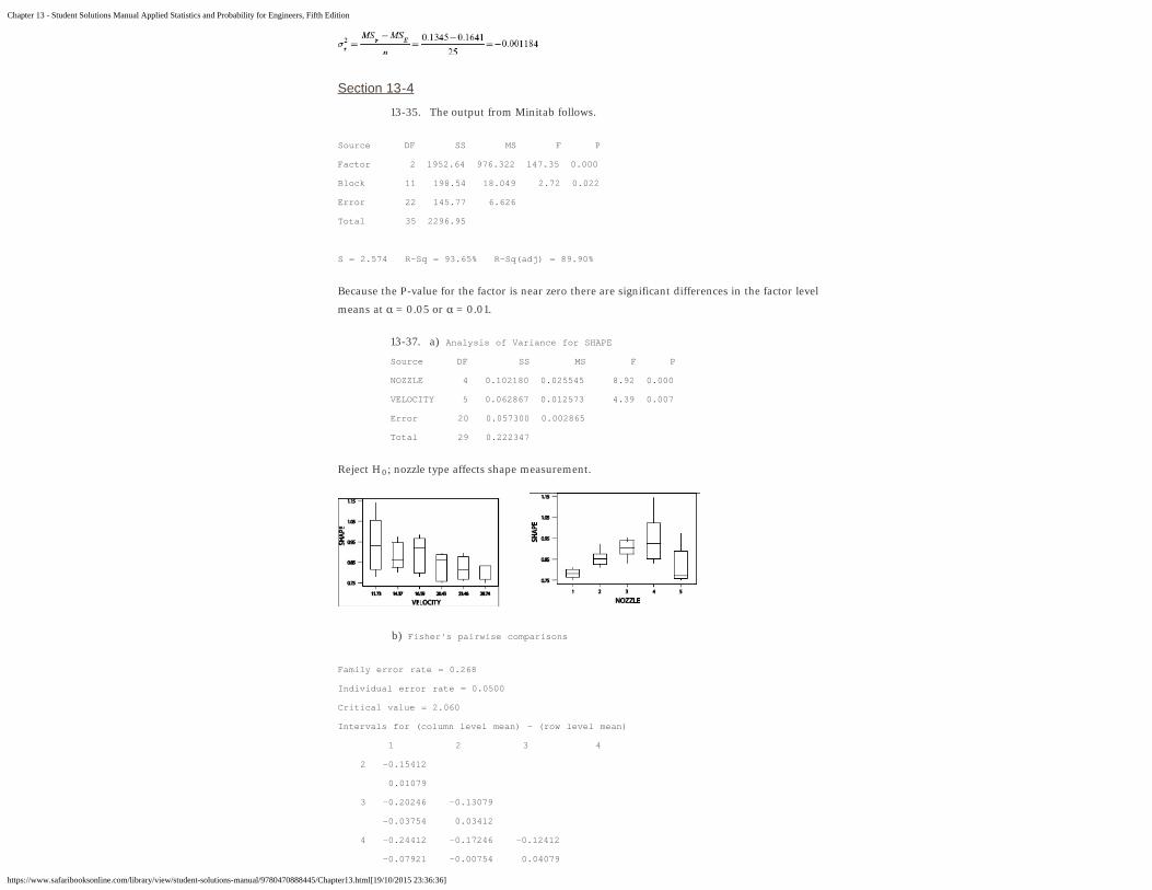
13-37. a) Analysis of Variance for SHAPE
Source DF SS MS F P
NOZZLE 4 0.102180 0.025545 8.92 0.000
VELOCITY 5 0.062867 0.012573 4.39 0.007
Error 20 0.057300 0.002865
Total 29 0.222347
Reject H ; nozzle type affects shape measurement.
b) Fisher's pairwise comparisons
Family error rate = 0.268
Individual error rate = 0.0500
Critical value = 2.060
Intervals for (column level mean) – (row level mean)
1 2 3 4
2 –0.15412
0.01079
3 –0.20246 –0.13079
–0.03754 0.03412
4 –0.24412 –0.17246 –0.12412
–0.07921 –0.00754 0.04079
0
Chapter 13 - Student Solutions Manual Applied Statistics and Probability for Engineers, Fifth Edition
https://www.safaribooksonline.com/library/view/student-solutions-manual/9780470888445/Chapter13.html[19/10/2015 23:36:36]
5 –0.11412 –0.04246 0.00588 0.04754
0.05079 0.12246 0.17079 0.21246
There are significant differences between levels 1 and 3; 4; 2 and 4; 3 and
5; and 4 and 5.
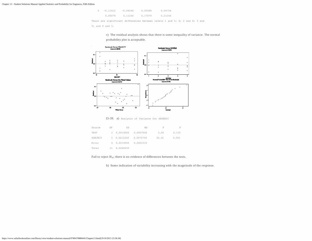
c) The residual analysis shows that there is some inequality of variance. The normal
probability plot is acceptable.
13-39. a) Analysis of Variance for ARSENIC
Source DF SS MS F P
TEST 2 0.0014000 0.0007000 3.00 0.125
SUBJECT 3 0.0212250 0.0070750 30.32 0.001
Error 6 0.0014000 0.0002333
Total 11 0.0240250
Fail to reject H ; there is no evidence of differences between the tests.
b) Some indication of variability increasing with the magnitude of the response.
0

Chapter 13 - Student Solutions Manual Applied Statistics and Probability for Engineers, Fifth Edition
https://www.safaribooksonline.com/library/view/student-solutions-manual/9780470888445/Chapter13.html[19/10/2015 23:36:36]
13-41. A version of the electronic data file has the reading for length 4 and width 5 as
2. It should be 20.
a) Analysis of Variance for LEAKAGE
Source DF SS MS F P
LENGTH 3 72.66 24.22 1.61 0.240
WIDTH 4 90.52 22.63 1.50 0.263
Error 12 180.83 15.07
Total 19 344.01
Fail to reject H , mean leakage voltage does not depend on the channel length.
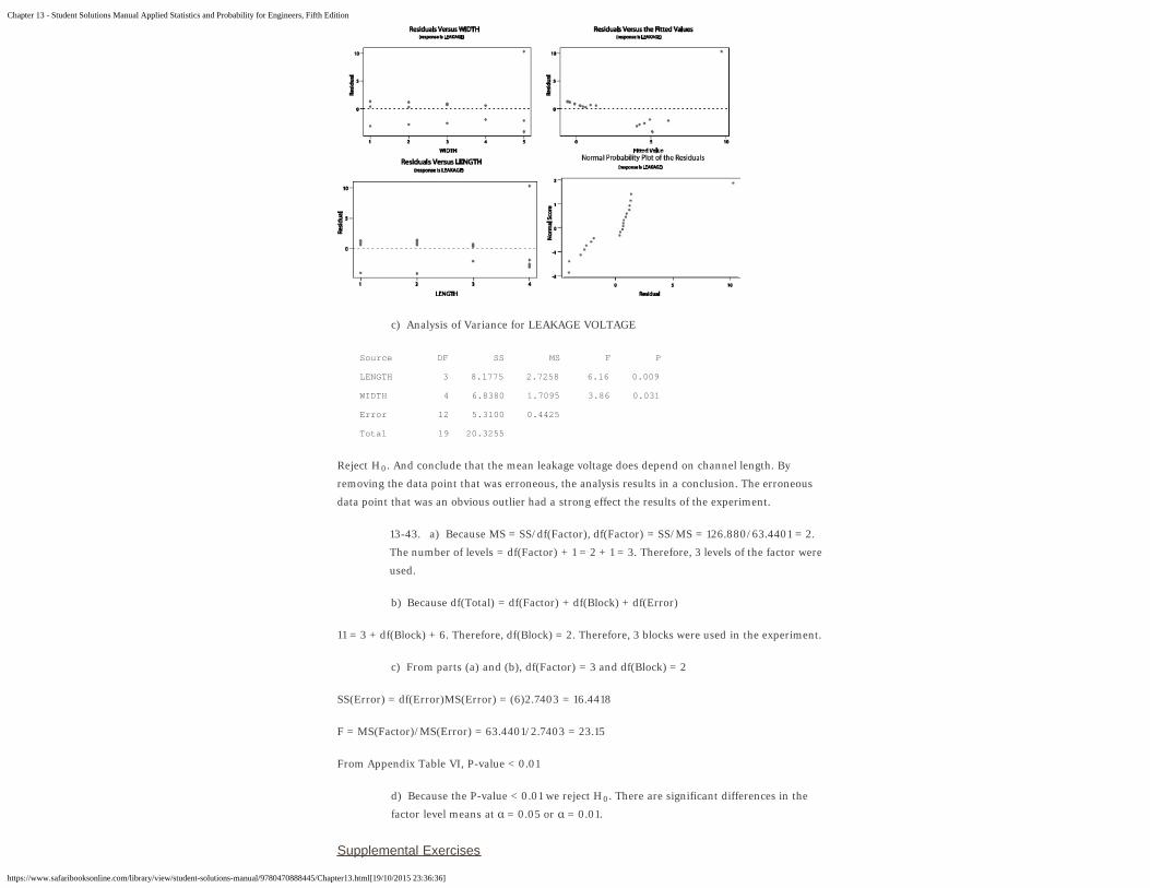
b) One unusual observation in width 5, length 4. There are some problems with the
normal probability plot, including the unusual observation.
0
Chapter 13 - Student Solutions Manual Applied Statistics and Probability for Engineers, Fifth Edition
https://www.safaribooksonline.com/library/view/student-solutions-manual/9780470888445/Chapter13.html[19/10/2015 23:36:36]
c) Analysis of Variance for LEAKAGE VOLTAGE
Source DF SS MS F P
LENGTH 3 8.1775 2.7258 6.16 0.009
WIDTH 4 6.8380 1.7095 3.86 0.031
Error 12 5.3100 0.4425
Total 19 20.3255
Reject H . And conclude that the mean leakage voltage does depend on channel length. By
removing the data point that was erroneous, the analysis results in a conclusion. The erroneous
data point that was an obvious outlier had a strong effect the results of the experiment.
13-43. a) Because MS = SS/df(Factor), df(Factor) = SS/MS = 126.880/63.4401 = 2.
The number of levels = df(Factor) + 1 = 2 + 1 = 3. Therefore, 3 levels of the factor were
used.
b) Because df(Total) = df(Factor) + df(Block) + df(Error)
11 = 3 + df(Block) + 6. Therefore, df(Block) = 2. Therefore, 3 blocks were used in the experiment.
c) From parts (a) and (b), df(Factor) = 3 and df(Block) = 2
SS(Error) = df(Error)MS(Error) = (6)2.7403 = 16.4418
F = MS(Factor)/MS(Error) = 63.4401/2.7403 = 23.15
From Appendix Table VI, P-value < 0.01
d) Because the P-value < 0.01 we reject H . There are significant differences in the
factor level means at α = 0.05 or α = 0.01.
Supplemental Exercises
0
0
Chapter 13 - Student Solutions Manual Applied Statistics and Probability for Engineers, Fifth Edition
https://www.safaribooksonline.com/library/view/student-solutions-manual/9780470888445/Chapter13.html[19/10/2015 23:36:36]
13-45. a) Analysis of Variance for RESISTANCE
Source DF SS MS F P
ALLOY 2 10941.8 5470.9 76.09 0.000
Error 27 1941.4 71.9
Total 29 12883.2
Reject H ; the type of alloy has a significant effect on mean contact resistance.
b) Fisher's pairwise comparisons
Family error rate = 0.119
Individual error rate = 0.0500
Critical value = 2.052
Intervals for (column level mean) – (row level mean)
1 2
2 –13.58
1.98
3 –50.88 –45.08
–35.32 –29.52
There are differences in the mean resistance for alloy types 1 and 3; and types 2 and 3.
c) 99% confidence interval on the mean contact resistance for alloy 3
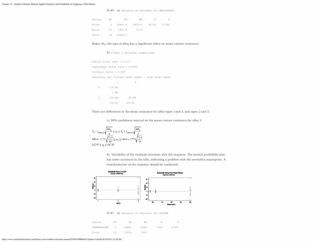
d) Variability of the residuals increases with the response. The normal probability plot
has some curvature in the tails, indicating a problem with the normality assumption. A
transformation of the response should be conducted.
13-47. a) Analysis of Variance for VOLUME
Source DF SS MS F P
TEMPERATURE 2 16480 8240 7.84 0.007
Error 12 12610 1051
0
Chapter 13 - Student Solutions Manual Applied Statistics and Probability for Engineers, Fifth Edition
https://www.safaribooksonline.com/library/view/student-solutions-manual/9780470888445/Chapter13.html[19/10/2015 23:36:36]
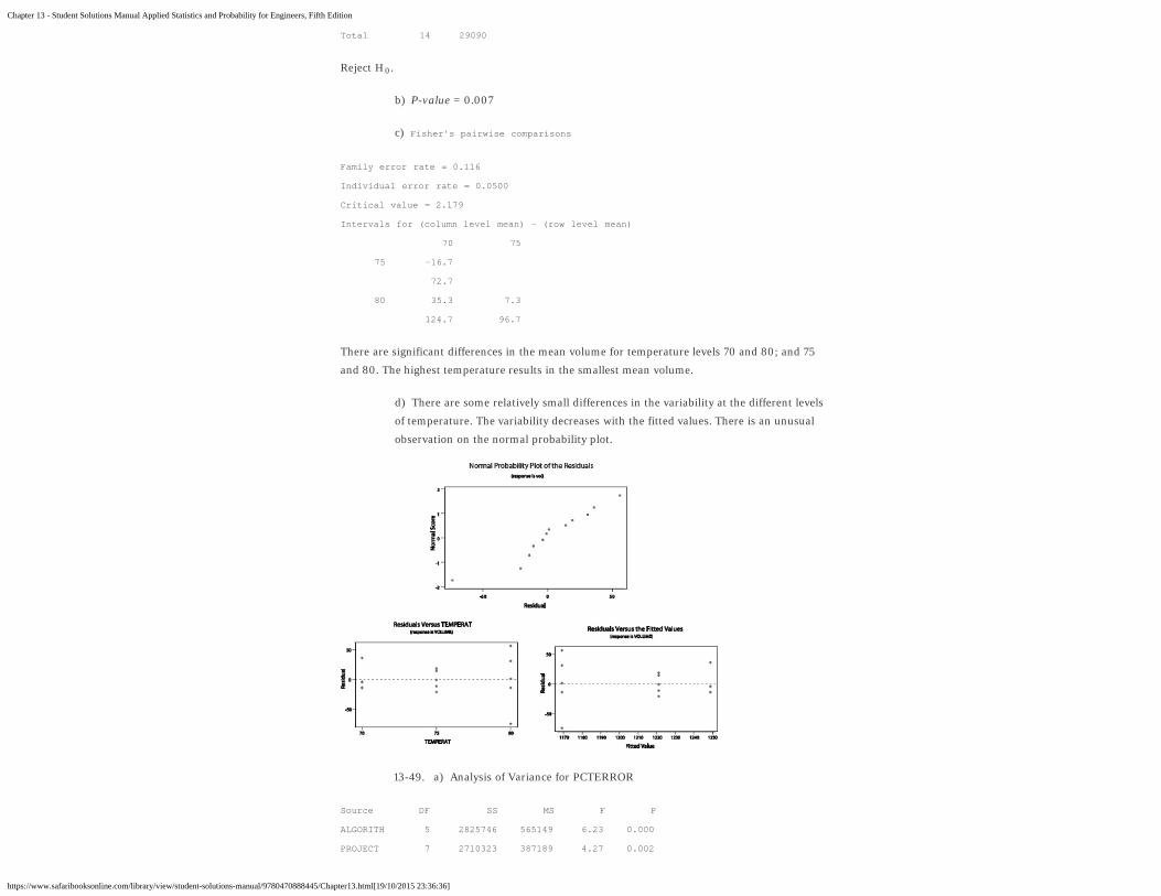
Total 14 29090
Reject H .
b) P-value = 0.007
c) Fisher's pairwise comparisons
Family error rate = 0.116
Individual error rate = 0.0500
Critical value = 2.179
Intervals for (column level mean) – (row level mean)
70 75
75 –16.7
72.7
80 35.3 7.3
124.7 96.7
There are significant differences in the mean volume for temperature levels 70 and 80; and 75
and 80. The highest temperature results in the smallest mean volume.
d) There are some relatively small differences in the variability at the different levels
of temperature. The variability decreases with the fitted values. There is an unusual
observation on the normal probability plot.
13-49. a) Analysis of Variance for PCTERROR
Source DF SS MS F P
ALGORITH 5 2825746 565149 6.23 0.000
PROJECT 7 2710323 387189 4.27 0.002
0
Chapter 13 - Student Solutions Manual Applied Statistics and Probability for Engineers, Fifth Edition
https://www.safaribooksonline.com/library/view/student-solutions-manual/9780470888445/Chapter13.html[19/10/2015 23:36:36]
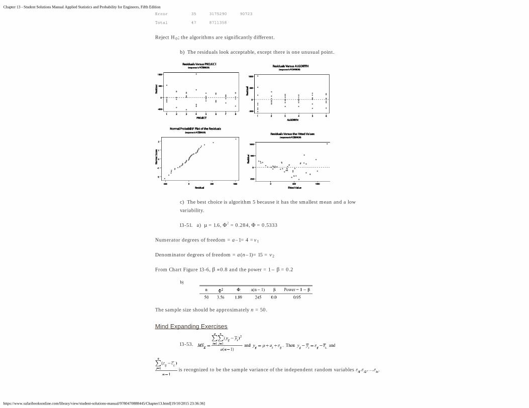
Error 35 3175290 90723
Total 47 8711358
Reject H ; the algorithms are significantly different.
b) The residuals look acceptable, except there is one unusual point.
c) The best choice is algorithm 5 because it has the smallest mean and a low
variability.
13-51. a) μ = 1.6, Φ = 0.284, Φ = 0.5333
Numerator degrees of freedom = a–1= 4 =v
Denominator degrees of freedom = a(n–1)= 15 = v
From Chart Figure 13-6, β ≈0.8 and the power = 1 – β = 0.2
The sample size should be approximately n = 50.
Mind Expanding Exercises
13-53.
is recognized to be the sample variance of the independent random variables .
0
1
2
2

Chapter 13 - Student Solutions Manual Applied Statistics and Probability for Engineers, Fifth Edition
https://www.safaribooksonline.com/library/view/student-solutions-manual/9780470888445/Chapter13.html[19/10/2015 23:36:36]
Therefore,
The development would not change if the random effects model had been specified because
for this model also.
13-55. is recognized as the sample standard
deviation calculated from
the data from population i. Then, which is the pooled variance estimate used in the t-
test.
13-57. If b, c, and d are the coefficients of three orthogonal contrasts, it can be shown
that
always holds. Upon dividing both sides by n,
we have which equals SS . The equation above can be obtained
from a
geometrical argument. The square of the distance of any point in four-dimensional space from the
zero point can be expressed as the sum of the squared distance along four orthogonal axes. Let
one of the axes be the 45 degree line and let the point be ( y , y , y , y ). The three orthogonal
contrasts are the other three axes. The square of the
distance of the point from the origin is and this equals the sum of the squared distances
along each of the
four axes.
13-59. Because is the sample
variance of
has a chi-square distribution with n – 1 degrees of freedom. Then,
is a sum of independent chi-square random variables. Consequently, has a chi-square
distribution with
a(n – 1) degrees of freedom. Consequently,
treatments
1. 2. 3. 4.
Chapter 13 - Student Solutions Manual Applied Statistics and Probability for Engineers, Fifth Edition
https://www.safaribooksonline.com/library/view/student-solutions-manual/9780470888445/Chapter13.html[19/10/2015 23:36:36]
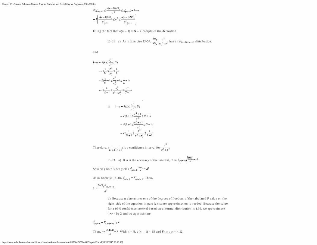
Using the fact that a(n – 1) = N – a completes the derivation.
13-61. a) As in Exercise 13-54, has an F distribution.
and
Therefore, is a confidence interval for
13-63. a) If A is the accuracy of the interval, then
Squaring both sides yields
As in Exercise 13-48, . Then,
b) Because n determines one of the degrees of freedom of the tabulated F value on the
right-side of the equation in part (a), some approximation is needed. Because the value
for a 95% confidence interval based on a normal distribution is 1.96, we approximate
by 2 and we approximate
Then, With n = 8, a(n – 1) = 35 and F = 4.12.
(a–1),(N–a)
0.05,1,35

Chapter 13 - Student Solutions Manual Applied Statistics and Probability for Engineers, Fifth Edition
https://www.safaribooksonline.com/library/view/student-solutions-manual/9780470888445/Chapter13.html[19/10/2015 23:36:36]
Recommended / Queue / Recent / Topics / Tutorials / Settings / Blog / Feedback / Sign Out /© 2015 Safari. Terms of Service / Privacy Policy
The value 4.12 can be used for F in the equation for n and a new value can be computed for n as
Because the solution for n did not change, we can use n = 8. If needed, another iteration could be
used to refine the value of n.
People who finished this also enjoyed:
Class Inheritancefrom: C++ Programming: Visual QuickStart Guide by Larry Ullman...Released: December 200553 MINS
C++ /
BOOK SECTION
Appendix C. Thermodynamic Tablesfrom: Modern Engineering Thermodynamics by Robert T. BalmerReleased: December 201015 MINS
Engineering /
BOOK SECTION
Object-Oriented Programmingfrom: Java, A Beginner’s Guide, 5th Edition by Herbert SchildtReleased: August 20117 MINS
Java /
BOOK SECTION
PREVChapter 12
NEXTChapter 14
https://www.safaribooksonline.com/library/view/student-solutions-manual/9780470888445/Chapter12.html
https://www.safaribooksonline.com/library/view/student-solutions-manual/9780470888445/Chapter12.html
https://www.safaribooksonline.com/library/view/student-solutions-manual/9780470888445/Chapter12.html
https://www.safaribooksonline.com/library/view/student-solutions-manual/9780470888445/Chapter14.html

Chapter 13 - Student Solutions Manual Applied Statistics and Probability for Engineers, Fifth Edition
https://www.safaribooksonline.com/library/view/student-solutions-manual/9780470888445/Chapter13.html[19/10/2015 23:36:36]