3. Probability and Statistics Applied to Hydrology · 3. Probability and Statistics Applied to...
48
3. Probability and Statistics Applied to Hydrology Chin - chapter 8 Dr. Luis E. Lesser All Tables and Figures (except where noted) were kindly provided by Pearson, from the textbook by David A. Chin, 2013. Water –Resources Engineering, 3 rd edition.
Transcript of 3. Probability and Statistics Applied to Hydrology · 3. Probability and Statistics Applied to...

3. Probability and Statistics Applied to Hydrology
Chin - chapter 8
Dr. Luis E. Lesser
All Tables and Figures (except where noted) were kindly provided by Pearson, from the
textbook by David A. Chin, 2013. Water –Resources Engineering, 3rd edition.
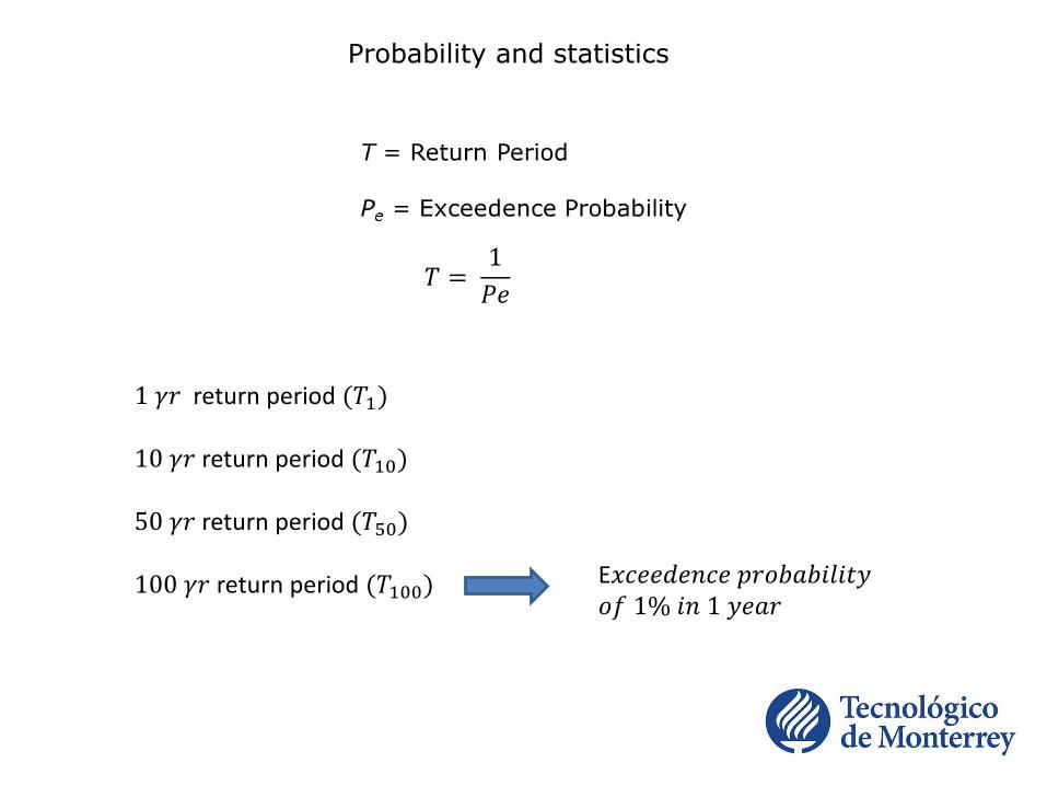
𝑇 =1
𝑃𝑒
Probability and statistics
1 𝛾𝑟 return period (𝑇1)
10 𝛾𝑟 return period (𝑇10)
50 𝛾𝑟 return period (𝑇50)
100 𝛾𝑟 return period (𝑇100)E𝑥𝑐𝑒𝑒𝑑𝑒𝑛𝑐𝑒 𝑝𝑟𝑜𝑏𝑎𝑏𝑖𝑙𝑖𝑡𝑦𝑜𝑓 1% 𝑖𝑛 1 𝑦𝑒𝑎𝑟
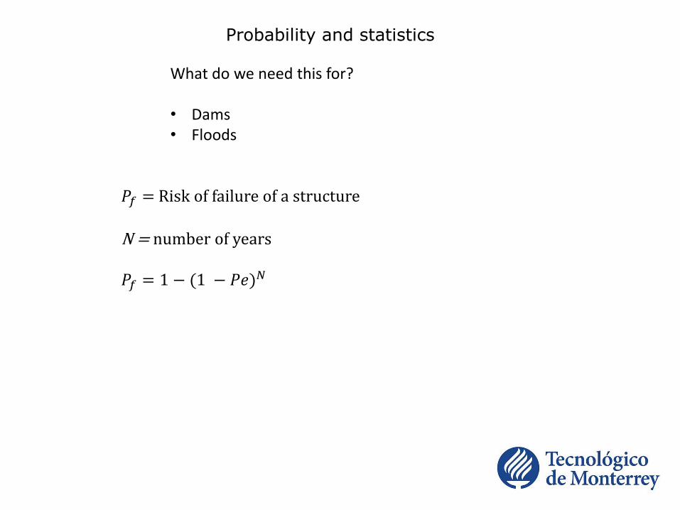
𝑃𝑓 = Risk of failure of a structure
N = number of years
𝑃𝑓 = 1 − (1 − 𝑃𝑒)𝑁
Probability and statistics
What do we need this for?
• Dams• Floods

Mean (average) 𝜇 different types (arithmetic, geometric)
Variance 𝜎2
𝜎 = 𝜎2
Standard deviation 𝜎
Discrete Σ
Distributions
Continuous ∫
Statistical parameters

Skewness
Data with skewness < 1 or >1 is greatly skewed
Graph from: wikipedia
Statistical parameters
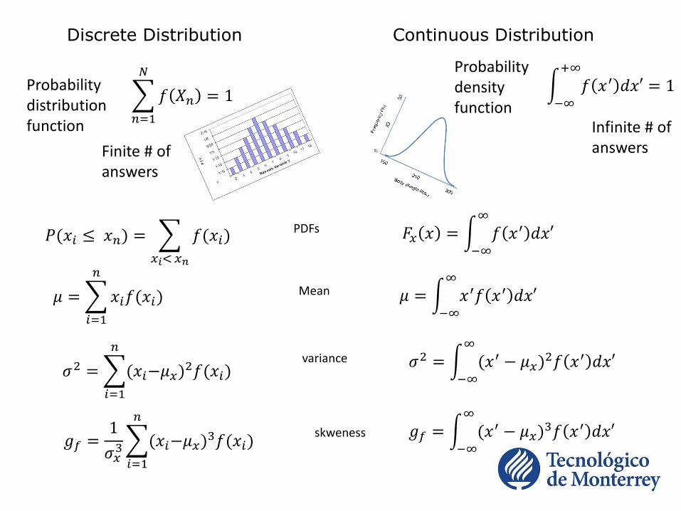
Discrete Distribution Continuous Distribution
Probabilitydistributionfunction
𝑃(𝑥𝑖 ≤ 𝑥𝑛) =
𝑥𝑖< 𝑥𝑛
𝑓(𝑥𝑖)
𝑛=1
𝑁
𝑓 𝑋𝑛 = 1
Finite # of answers
Probabilitydensityfunction
−∞
+∞
𝑓 𝑥′ 𝑑𝑥′ = 1
Infinite # of answers
𝐹𝑥 𝑥 = −∞
∞
𝑓 𝑥′ 𝑑𝑥′
𝜇 =
𝑖=1
𝑛
𝑥𝑖𝑓(𝑥𝑖)
𝜎2 =
𝑖=1
𝑛
(𝑥𝑖−𝜇𝑥)2𝑓(𝑥𝑖)
𝑔𝑓 =1
𝜎𝑥3
𝑖=1
𝑛
(𝑥𝑖−𝜇𝑥)3𝑓(𝑥𝑖)
𝜇 = −∞
∞
𝑥′𝑓 𝑥′ 𝑑𝑥′
𝜎2 = −∞
∞
(𝑥′ − 𝜇𝑥)2𝑓 𝑥′ 𝑑𝑥′
𝑔𝑓 = −∞
∞
(𝑥′ − 𝜇𝑥)3𝑓 𝑥′ 𝑑𝑥′
variance
skweness
Mean
PDFs
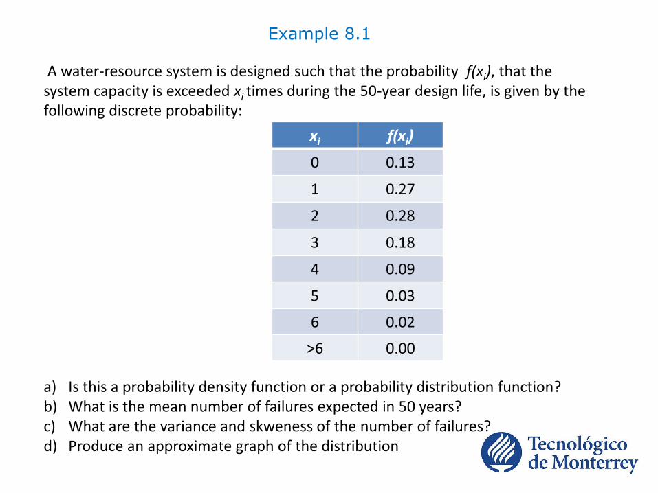
Example 8.1
A water-resource system is designed such that the probability f(xi), that the system capacity is exceeded xi times during the 50-year design life, is given by the following discrete probability:
a) Is this a probability density function or a probability distribution function?b) What is the mean number of failures expected in 50 years? c) What are the variance and skweness of the number of failures?d) Produce an approximate graph of the distribution
xi f(xi)
0 0.13
1 0.27
2 0.28
3 0.18
4 0.09
5 0.03
6 0.02
>6 0.00
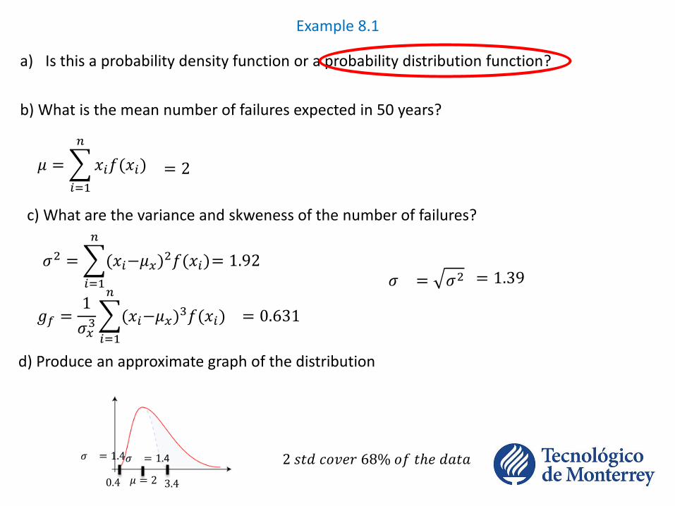
Example 8.1
a) Is this a probability density function or a probability distribution function?
c) What are the variance and skweness of the number of failures?
b) What is the mean number of failures expected in 50 years?
𝜇 =
𝑖=1
𝑛
𝑥𝑖𝑓(𝑥𝑖) = 2
𝜎2 =
𝑖=1
𝑛
(𝑥𝑖−𝜇𝑥)2𝑓(𝑥𝑖)
𝑔𝑓 =1
𝜎𝑥3
𝑖=1
𝑛
(𝑥𝑖−𝜇𝑥)3𝑓(𝑥𝑖)
= 1.92
= 0.631
d) Produce an approximate graph of the distribution
𝜇 = 20.4
𝜎 = 1.4𝜎 = 1.4
3.4
2 𝑠𝑡𝑑 𝑐𝑜𝑣𝑒𝑟 68% 𝑜𝑓 𝑡ℎ𝑒 𝑑𝑎𝑡𝑎
𝜎 = 𝜎2 = 1.39

1 − 𝑃
Return Period
𝑇 =1
𝑃𝑒where 𝑃𝑒 is exceedance probability
𝑃𝑒 =1
𝑇
100 𝑦𝑟 𝐹𝑙𝑜𝑜𝑑
Cumulative Probability
Remember:
𝑃 𝑋 > 𝑋𝑇 =1
𝑇
20 𝑦𝑟 𝐹𝑙𝑜𝑜𝑑
exceedance probability 𝑜𝑓1
100
exceedance probability 𝑜𝑓1
20
= 1% in any given 𝑦𝑟
= 5% in any given 𝑦𝑟
𝑃 𝑋 > 𝑋𝑇 = 𝑃
𝑃 𝑋 < 𝑋𝑇 =

Example 8.3
Analyses of the maximum-annual floods over the past 150 years in a small river indicate the following cumulative distribution
Flow, Xn
(m3/s)P(X<xn)
0 025 0.1950 0.3575 0.52
100 0.62125 0.69150 0.88175 0.92200 0.95225 0.98250 1.00
a) Estimate the magnitude of the flood with a return period of 10 years
a) Estimate the magnitude of the flood with a return period of 10 years
b) Estimate the magnitudes of the floods with return periods of: Yellow – 20 years Orange – 35 years Blue – 50 years Green – 100 years

PROBABILITY FUNCTIONS
1. Binomial Distribution or Bernoulli Distribution
• It is a discrete probability distribution
• Describes mathematically success or failure (coin toss)
• The outcome of any trial is independent of any other trial
𝐵𝑖𝑛𝑜𝑚𝑖𝑎𝑙 𝐷𝑖𝑠𝑡𝑟𝑖𝑏𝑢𝑡𝑖𝑜𝑛 = 𝑓𝑛 =𝑁𝑛
𝑃𝑛 1 − 𝑃 𝑁−𝑛
P = probability of success
n = number of successes
N = number of trials
𝑁𝑛
= 𝑝𝑒𝑟𝑚𝑢𝑡𝑎𝑡𝑖𝑜𝑛𝑠 =𝑁!
𝑛! 𝑁 − 𝑛 !
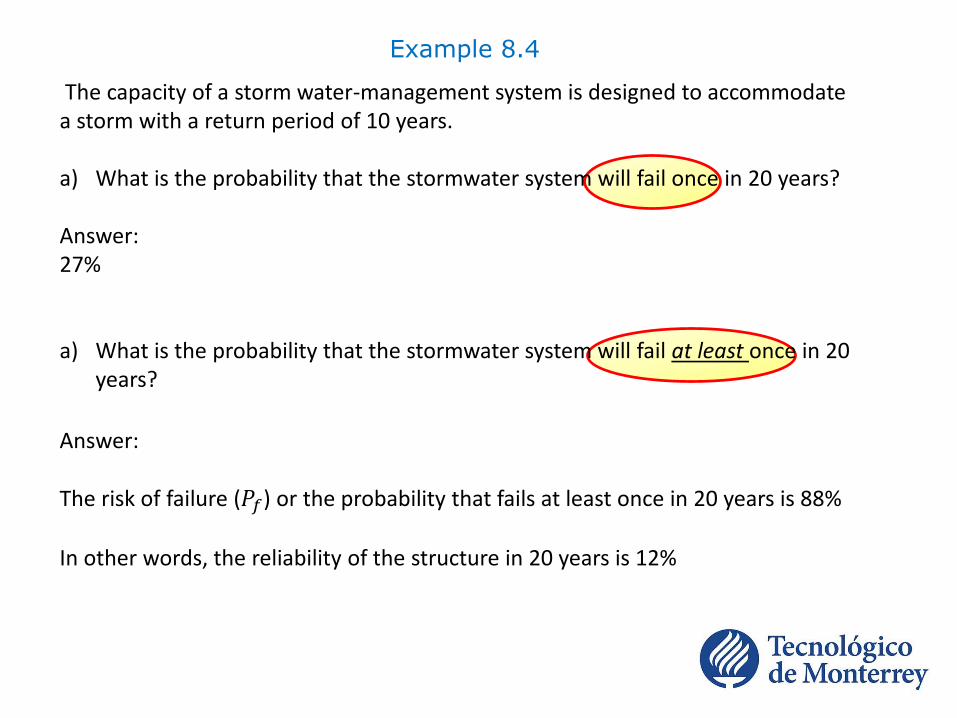
Example 8.4
The capacity of a storm water-management system is designed to accommodate a storm with a return period of 10 years.
a) What is the probability that the stormwater system will fail once in 20 years?
Answer: 27%
a) What is the probability that the stormwater system will fail at least once in 20 years?
Answer:
The risk of failure (𝑃𝑓) or the probability that fails at least once in 20 years is 88%
In other words, the reliability of the structure in 20 years is 12%

2. Poisson Distribution
• Is a limiting case of Bernoulli Distribution in which the expected number of successes (𝑁 ∗ 𝑃) is constant
• The number of trials (N) is large and the probability of success (P) in each trial diminishes
Examples: Large earthquake in Mexico City→ 20 years with no eventReturn period → 10 years with no event
𝑃 = 𝑓 𝑛 =𝜆𝑛𝑒−𝜆
𝑛!
𝜆 = expected number of successes = 𝑁 ∗ 𝑃
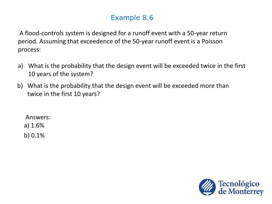
Example 8.6
A flood-controls system is designed for a runoff event with a 50-year return period. Assuming that exceedence of the 50-year runoff event is a Poisson process:
a) What is the probability that the design event will be exceeded twice in the first 10 years of the system?
Answers:a) 1.6%
b) 0.1%
b) What is the probability that the design event will be exceeded more than twice in the first 10 years?
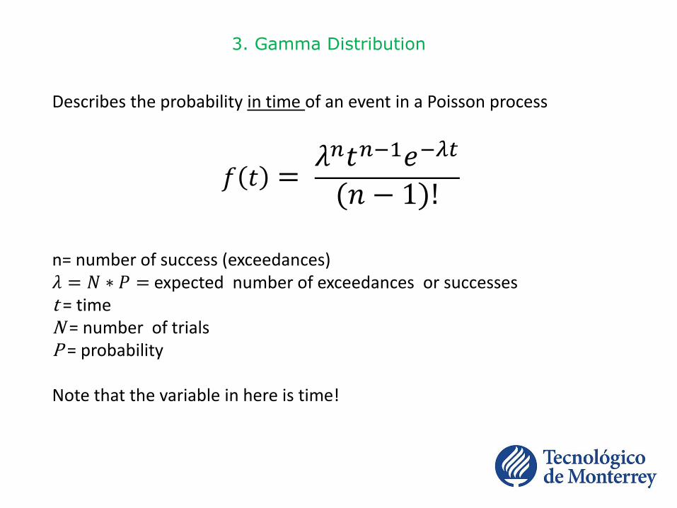
3. Gamma Distribution
Describes the probability in time of an event in a Poisson process
n= number of success (exceedances)𝜆 = 𝑁 ∗ 𝑃 = expected number of exceedances or successest = timeN = number of trialsP = probability
Note that the variable in here is time!
𝑓 𝑡 =𝜆𝑛𝑡𝑛−1𝑒−𝜆𝑡
𝑛 − 1 !

3. Gamma Distribution
𝜇𝑡 =𝑛
𝜆
When n is not an integer, then:
generally used for skewed variables
𝜎𝑡2 =
𝑛
𝜆2 𝑔𝑡 =2
𝑛
𝑓 𝑡 =𝜆𝑛𝑡𝑛−1𝑒−𝜆𝑡
Γ(𝑛)
Γ(𝑛) = 0
∞
𝑡𝑛−1𝑒−1 𝑑𝑡 Γ(𝑛) =(n-1)! For n = 1,2,3…
time
Gamma Function

4. Pearson III Distribution (or Gama III Distribution)
Similar to Gamma Distribution
𝑃(𝑥) =𝜆𝛽(𝑋 − 𝜖)𝛽−1𝑒−𝜆(𝑥−𝜖)
Γ(𝛽)
𝛽 =2
𝑔𝑥
2
𝜆 =𝛽
𝜎𝑥𝜖 = 𝜇𝑥 −
𝛽
𝜆
• Used for distribution of annual-maximum flood peaks
• Widely used in China
5. Log-Pearson Type III or LP3 Distribution
• It is the log of the Gama III Distribution
• It is also called Log-Pearson Type III Distribution or LP3
• Officially recommended by the U.S. Interagency Advisory Committee on Water Data by the ASCE (1980)

6. Normal Distribution or Gaussian Distribution
Symetrical, bell-shaped
Standard Normal Deviate (Z):
𝑓(𝑥) =1
𝜎𝑥 2𝜋𝑒𝑥𝑝 −
1
2
𝑥 − 𝜇𝑥𝜎𝑥
2
𝑧 =𝑥 − 𝜇𝑥
𝜎𝑥
𝐵 =1
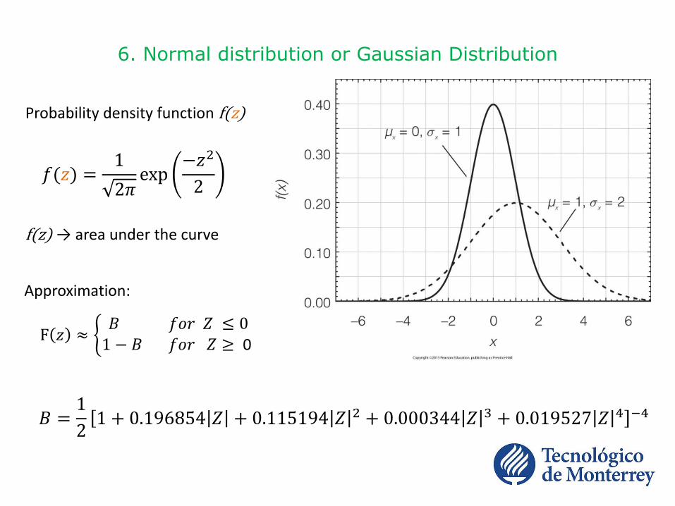
21 + 0.196854 𝑍 + 0.115194 𝑍 2 + 0.000344 𝑍 3 + 0.019527 𝑍 4 −4
6. Normal distribution or Gaussian Distribution
Probability density function f(z)
f(z) → area under the curve
𝑓(𝑧) =1
2𝜋exp
−𝑧2
2
F 𝑧 ≈ 𝐵 𝑓𝑜𝑟 𝑍 ≤ 01 − 𝐵 𝑓𝑜𝑟 𝑍 ≥ 0
Approximation:
Example 8.9
The annual rainfall in the Upper Kissimmee River basin has been estimated to have a mean of 130 cm and a standard deviation of 15.6 cm. Assuming that the annual rainfall is normally distributed, what is the probability of having an annual rainfall of less than 101.6 cm?
Answer:3.4%

7. Log Normal Distribution
𝑌 = ln𝑋
𝑓 𝑥 =1
𝑥𝜎𝑦 2𝜋𝑒𝑥𝑝 −
(ln 𝑥 − 𝜇𝑦)2
2𝜎𝑦2 𝑓𝑜𝑟 𝑥 > 0
Where:
𝜇𝑥 = exp(𝜇𝑦 +𝜎𝑦2
2)
𝜎𝑥2 = 𝜇𝑥
2[exp(𝜎𝑦2) − 1]
𝑔𝑥 = 3𝐶𝑣 + 𝐶𝑣3
𝐶𝑣= Coefficient of variation 𝐶𝑣 =𝜎𝑥𝜇𝑥
Z=𝑦−𝜇𝑦
𝜎𝑦
𝜇𝑦 ≠ 𝑙𝑛𝜇𝑥
∴ we will transform the variable X into the variable Y and calculate Z in terms of Y
Example 8.10
Annual-maximum discharges in the Guadalupe River show a mean of 801 m3/s and a standard deviation of 851 m3/s. If the capacity of the river channel is 900 m3/s, and the flow is assumed to follow a log-normal distribution, what is the probability that the maximum discharge will exceed the channel capacity?
Answer:There is a 28.6% of probability of flooding on any given year
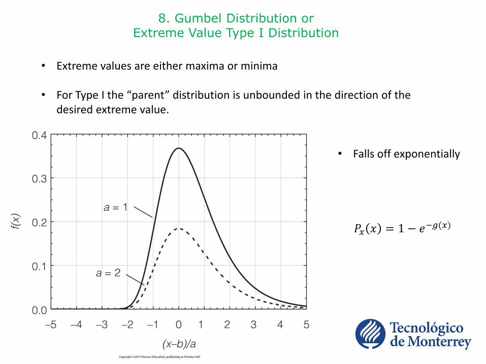
• Extreme values are either maxima or minima
• For Type I the “parent” distribution is unbounded in the direction of the desired extreme value.
8. Gumbel Distribution or Extreme Value Type I Distribution
𝑃𝑥 𝑥 = 1 − 𝑒−𝑔(𝑥)
• Falls off exponentially
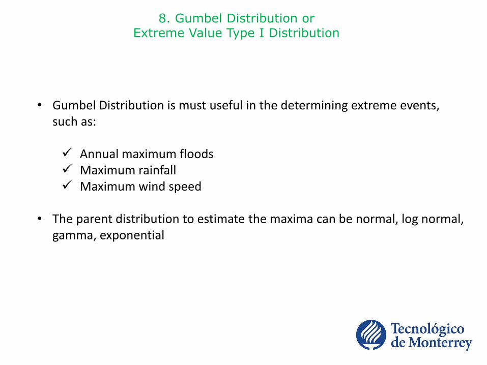
• Gumbel Distribution is must useful in the determining extreme events, such as:
Annual maximum floods Maximum rainfall Maximum wind speed
• The parent distribution to estimate the maxima can be normal, log normal, gamma, exponential
8. Gumbel Distribution or Extreme Value Type I Distribution
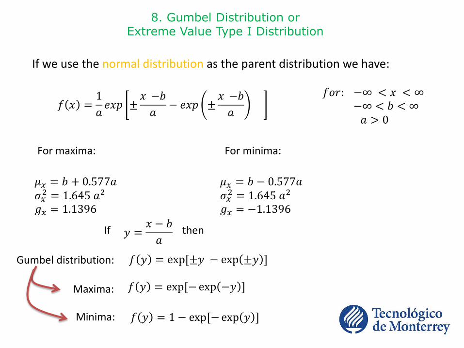
For maxima: For minima:
𝜇𝑥 = 𝑏 + 0.577𝑎𝜎𝑥2 = 1.645 𝑎2
𝑔𝑥 = 1.1396
𝜇𝑥 = 𝑏 − 0.577𝑎𝜎𝑥2 = 1.645 𝑎2
𝑔𝑥 = −1.1396
𝑓 𝑦 = exp[±𝑦 − exp ±𝑦 ]
𝑓 𝑦 = exp[−exp −𝑦 ]
𝑓 𝑦 = 1 − exp[−exp 𝑦 ]
8. Gumbel Distribution or Extreme Value Type I Distribution
If we use the normal distribution as the parent distribution we have:
𝑓 𝑥 =1
𝑎𝑒𝑥𝑝 ±
𝑥 −𝑏
𝑎− 𝑒𝑥𝑝 ±
𝑥 −𝑏
𝑎
𝑓𝑜𝑟: −∞ < 𝑥 < ∞−∞ < 𝑏 < ∞𝑎 > 0
Gumbel distribution:
Maxima:
If then𝑦 =𝑥 − 𝑏
𝑎
Minima:
Example 8.12
The annual-maximum discharges in the Guadalupe River between 1935 and 1978 show a mean of 811 m3/s and a standard deviation of 851 m3/s. Assuming that the annual-maximum flows are described by an extreme-value Type I (Gumbel) distribution, estimate the annual-maximum flowrate with a return period of 100 years.
Answer:A flow of 3,482 m3/s has a return period of 100 years
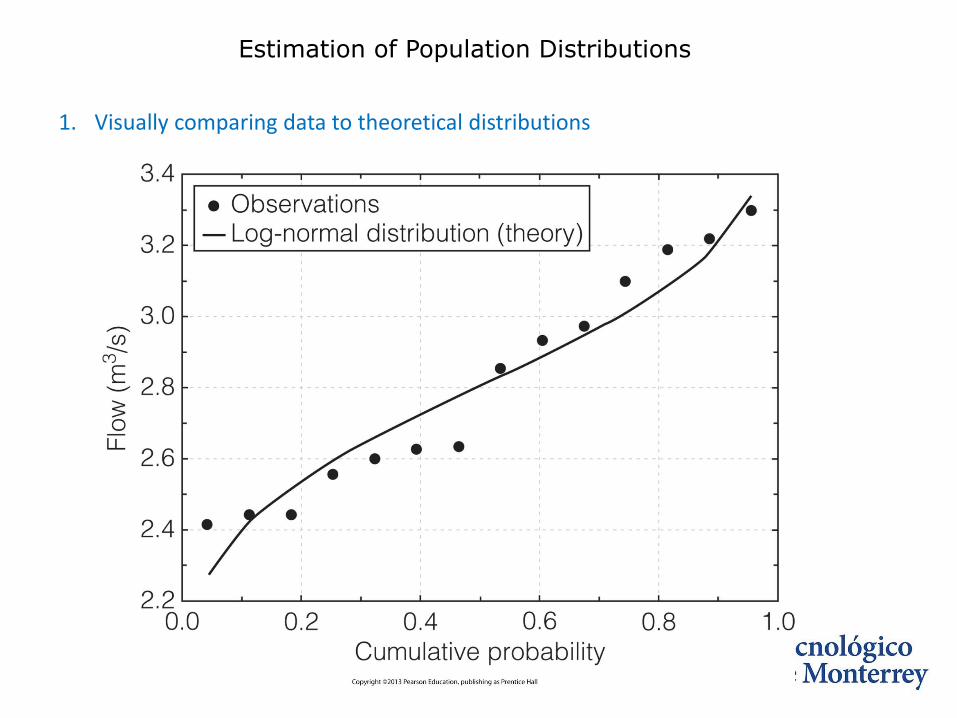
Estimation of Population Distributions
1. Visually comparing data to theoretical distributions
Estimation of Population Distributions
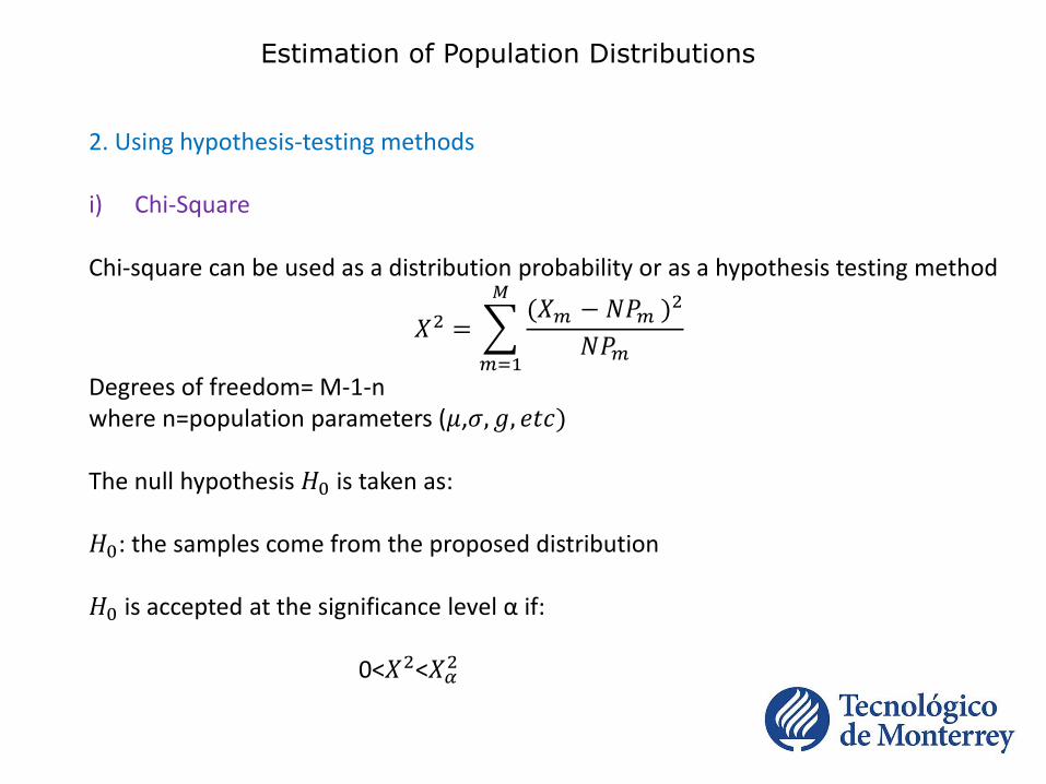
2. Using hypothesis-testing methods
i) Chi-Square
Chi-square can be used as a distribution probability or as a hypothesis testing method
𝑋2 =
𝑚=1
𝑀(𝑋𝑚 − 𝑁𝑃𝑚 )2
𝑁𝑃𝑚
Degrees of freedom= M-1-nwhere n=population parameters (𝜇,𝜎, 𝑔, 𝑒𝑡𝑐)
The null hypothesis 𝐻0 is taken as:
𝐻0: the samples come from the proposed distribution
𝐻0 is accepted at the significance level α if:
0<𝑋2<𝑋𝛼2
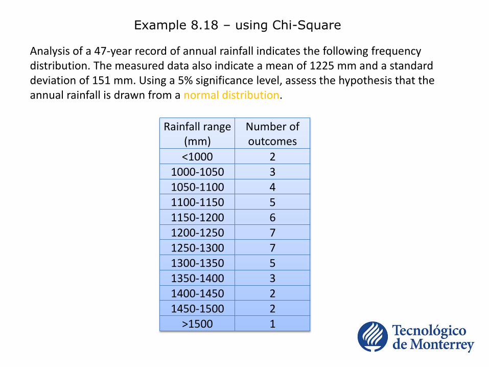
Example 8.18 – using Chi-Square
Analysis of a 47-year record of annual rainfall indicates the following frequency distribution. The measured data also indicate a mean of 1225 mm and a standard deviation of 151 mm. Using a 5% significance level, assess the hypothesis that the annual rainfall is drawn from a normal distribution.
Rainfall range (mm)
Number of outcomes
<1000 21000-1050 31050-1100 41100-1150 51150-1200 61200-1250 71250-1300 71300-1350 51350-1400 31400-1450 21450-1500 2
>1500 1
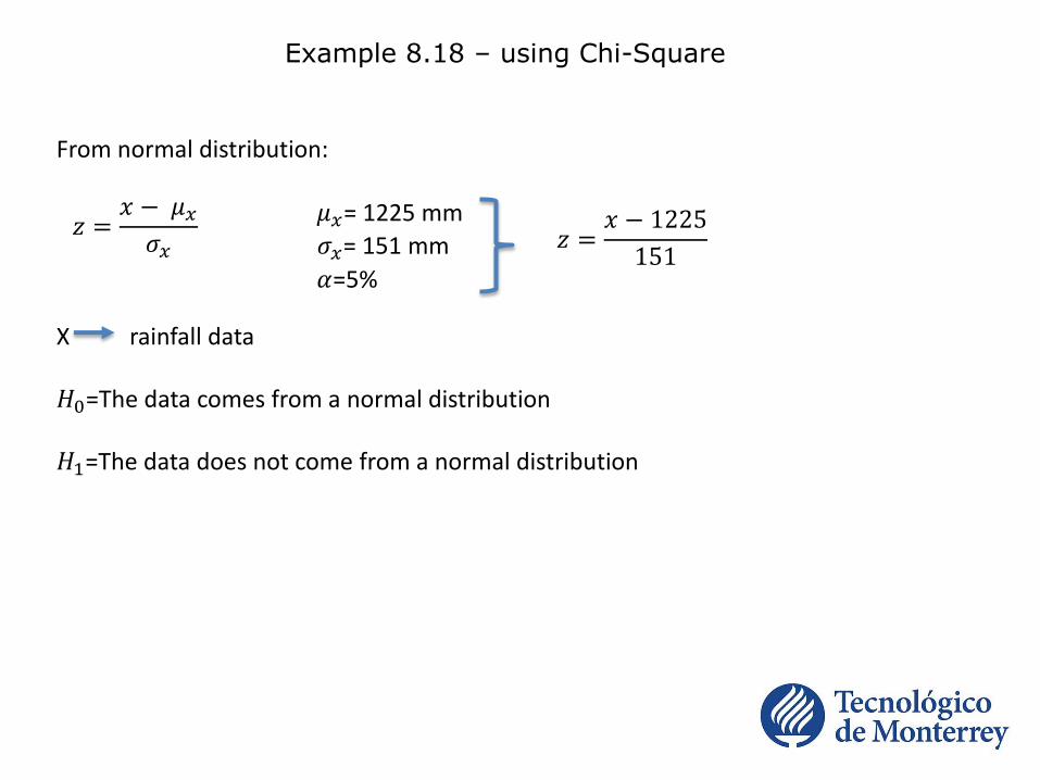
Example 8.18 – using Chi-Square
From normal distribution:
X rainfall data
𝐻0=The data comes from a normal distribution
𝐻1=The data does not come from a normal distribution
𝑧 =𝑥 − 𝜇𝑥
𝜎𝑥
𝜇𝑥= 1225 mm
𝜎𝑥= 151 mm
𝛼=5%
𝑧 =𝑥 − 1225
151
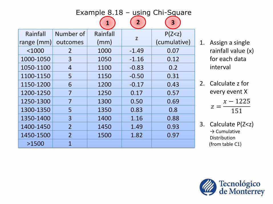
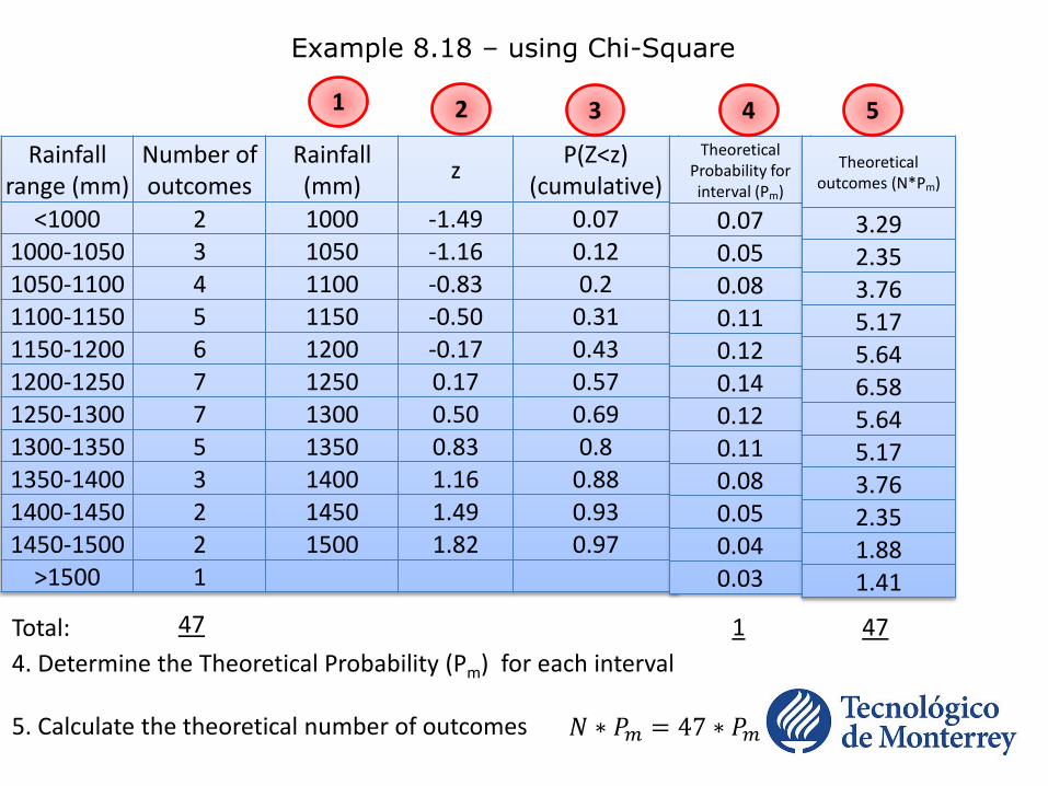
Example 8.18 – using Chi-Square
Rainfallrange (mm)
Number of outcomes
Rainfall (mm)
zP(Z<z)
(cumulative)
<1000 2 1000 -1.49 0.071000-1050 3 1050 -1.16 0.121050-1100 4 1100 -0.83 0.21100-1150 5 1150 -0.50 0.311150-1200 6 1200 -0.17 0.431200-1250 7 1250 0.17 0.571250-1300 7 1300 0.50 0.691300-1350 5 1350 0.83 0.81350-1400 3 1400 1.16 0.881400-1450 2 1450 1.49 0.931450-1500 2 1500 1.82 0.97
>1500 1
2 3
1. Assign a single rainfall value (x) for each data interval
2. Calculate z for every event X
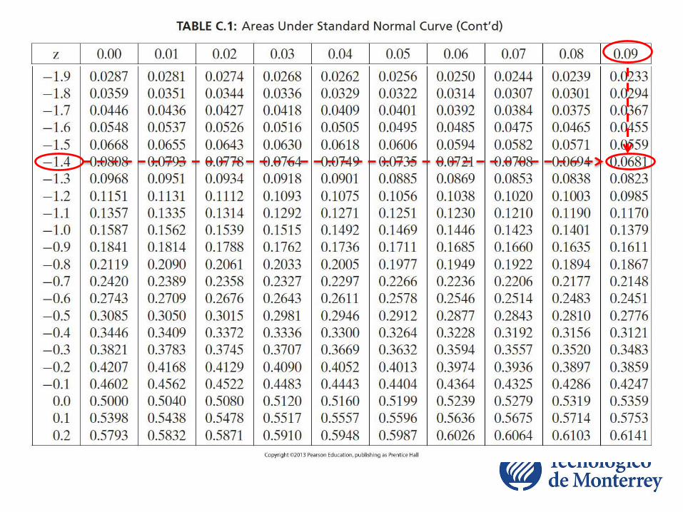
3. Calculate P(Z<z) → Cumulative Distribution(from table C1)
𝑧 =𝑥 − 1225
151
1

Example 8.18 – using Chi-Square
Rainfall range (mm)
Number of outcomes
Rainfall (mm)
zP(Z<z)
(cumulative)
<1000 2 1000 -1.49 0.071000-1050 3 1050 -1.16 0.121050-1100 4 1100 -0.83 0.21100-1150 5 1150 -0.50 0.311150-1200 6 1200 -0.17 0.431200-1250 7 1250 0.17 0.571250-1300 7 1300 0.50 0.691300-1350 5 1350 0.83 0.81350-1400 3 1400 1.16 0.881400-1450 2 1450 1.49 0.931450-1500 2 1500 1.82 0.97
>1500 1
Theoretical Probability for interval (Pm)
0.070.050.080.110.120.140.120.110.080.050.040.03
Theoretical outcomes (N*Pm)
3.292.353.765.175.646.585.645.173.762.351.881.41
2 543
Total: 47 471
1
4. Determine the Theoretical Probability (Pm) for each interval
5. Calculate the theoretical number of outcomes 𝑁 ∗ 𝑃𝑚 = 47 ∗ 𝑃𝑚
Example 8.18 – using Chi-Square
Rainfall range (mm)
Number of outcomes
Rainfall (mm)
zP(Z<z)
(cumulative)
<1000 2 1000 -1.49 0.071000-1050 3 1050 -1.16 0.121050-1100 4 1100 -0.83 0.21100-1150 5 1150 -0.50 0.311150-1200 6 1200 -0.17 0.431200-1250 7 1250 0.17 0.571250-1300 7 1300 0.50 0.691300-1350 5 1350 0.83 0.81350-1400 3 1400 1.16 0.881400-1450 2 1450 1.49 0.931450-1500 2 1500 1.82 0.97
>1500 1
Theoretical Probability for interval (Pm)
0.070.050.080.110.120.140.120.110.080.050.040.03
Theoretical outcomes (N*Pm)
3.292.353.765.175.646.585.645.173.762.351.881.41
2 543
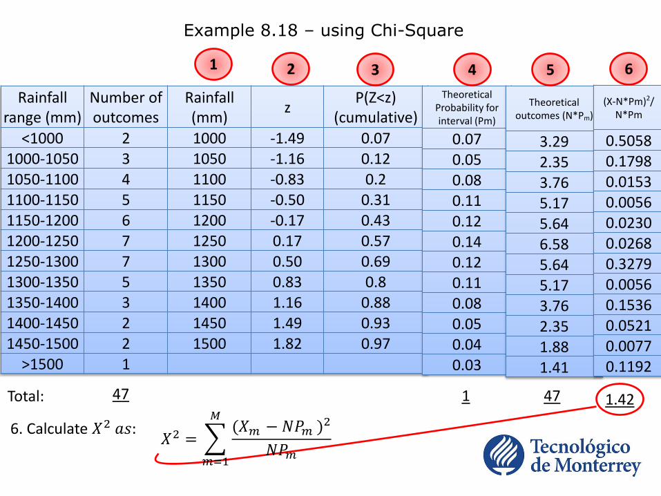
(X-N*Pm)2/N*Pm
0.50580.17980.01530.00560.02300.02680.32790.00560.15360.05210.00770.1192
6
Total: 47 471 1.42
1
6. Calculate 𝑋2 𝑎𝑠:𝑋2 =
𝑚=1
𝑀(𝑋𝑚 − 𝑁𝑃𝑚 )2
𝑁𝑃𝑚
Example 8.18 – using Chi-Square
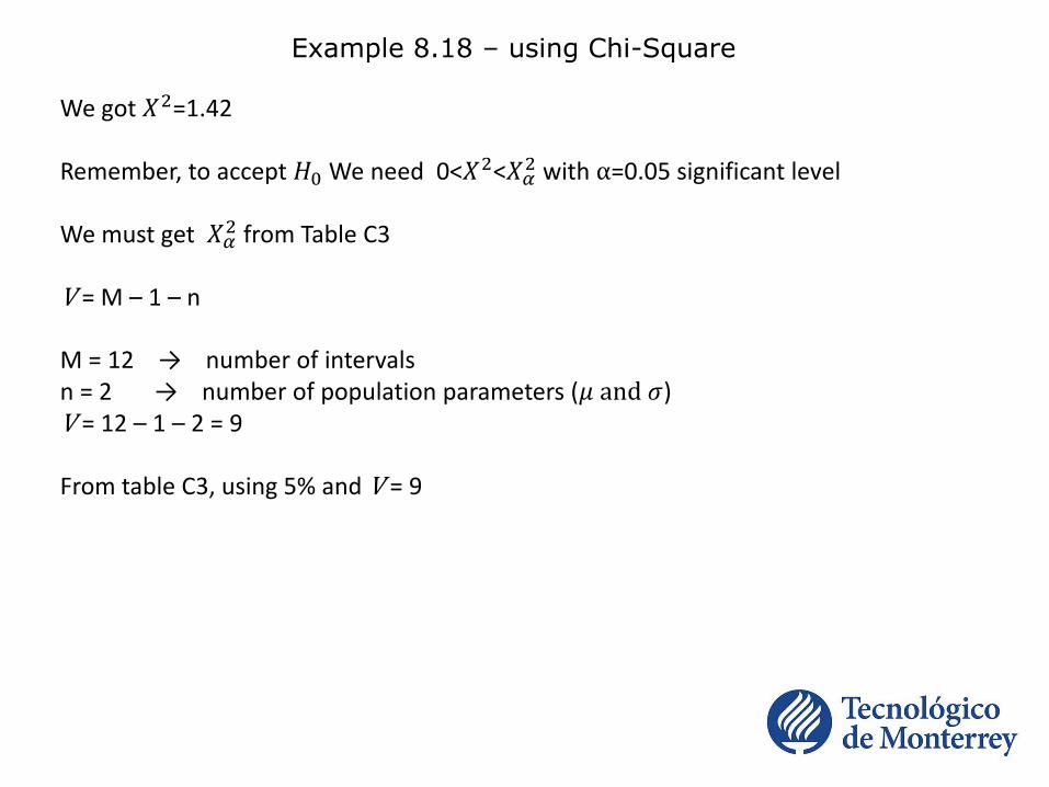
We got 𝑋2=1.42
Remember, to accept 𝐻0 We need 0<𝑋2<𝑋𝛼2 with α=0.05 significant level
We must get 𝑋𝛼2 from Table C3
V = M – 1 – n
M = 12 → number of intervalsn = 2 → number of population parameters (𝜇 and 𝜎)V = 12 – 1 – 2 = 9
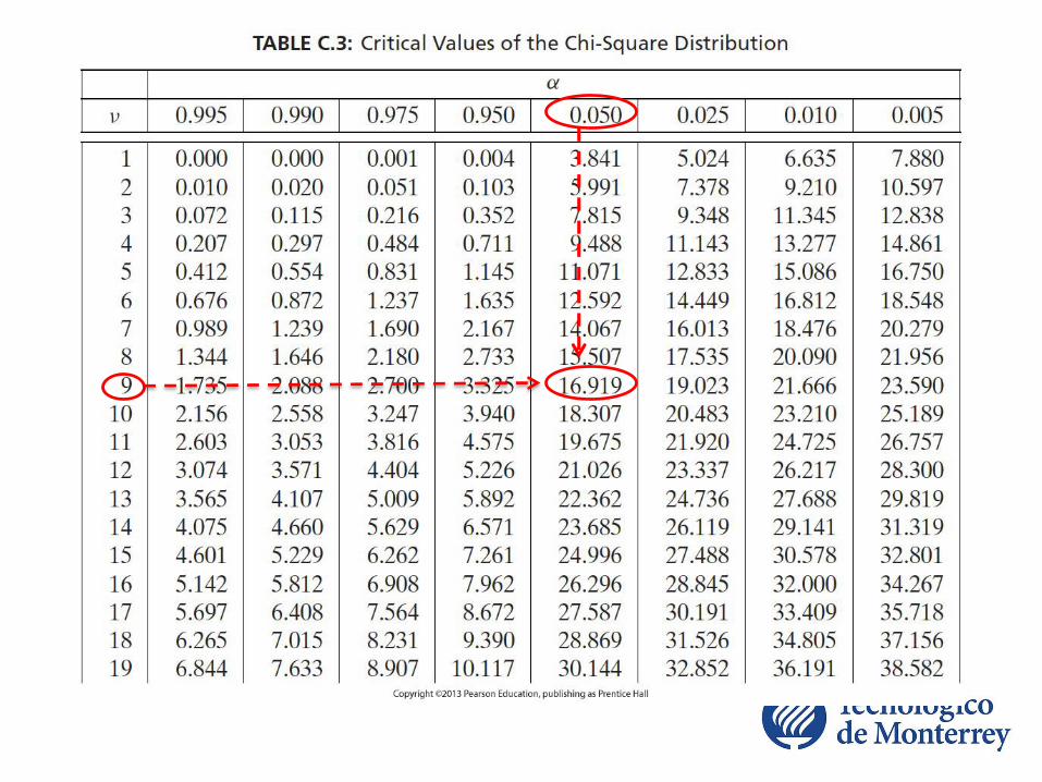
From table C3, using 5% and V = 9
Example 8.18 – using Chi-Square
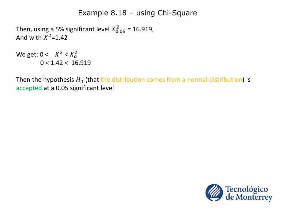
Then, using a 5% significant level 𝑋0.052 = 16.919,
And with 𝑋2=1.42
We get: 0 < 𝑋2 < 𝑋𝛼2
0 < 1.42 < 16.919
Then the hypothesis 𝐻0 (that the distribution comes from a normal distribution) is accepted at a 0.05 significant level

ii) Kolmogorov-Smirnov test
Another hypothesis testing method to determine the distribution
If the calculated D value is less than (<) the critical Ks value, then 𝐻0 is accepted
Example 8.19:
Use the Kolmogorov-Smirnov test at the 10% significance level to assess the hypothesis that the data from example 8.18 are drawn from a normal distribution
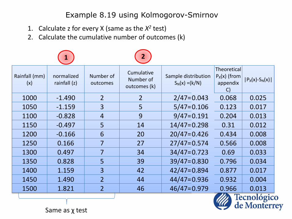
Example 8.19 using Kolmogorov-Smirnov
Rainfall (mm) (x)
normalized rainfall (z)
Number of outcomes
Cumulative Number of
outcomes (k)
Sample distribution SN(x) =(k/N)
TheoreticalPX(x) (from appendix
C)
|PX(x)-SN(x)|
1000 -1.490 2 2 2/47=0.043 0.068 0.0251050 -1.159 3 5 5/47=0.106 0.123 0.0171100 -0.828 4 9 9/47=0.191 0.204 0.0131150 -0.497 5 14 14/47=0.298 0.31 0.0121200 -0.166 6 20 20/47=0.426 0.434 0.0081250 0.166 7 27 27/47=0.574 0.566 0.0081300 0.497 7 34 34/47=0.723 0.69 0.0331350 0.828 5 39 39/47=0.830 0.796 0.0341400 1.159 3 42 42/47=0.894 0.877 0.0171450 1.490 2 44 44/47=0.936 0.932 0.0041500 1.821 2 46 46/47=0.979 0.966 0.013
Same as χ test
1 2
1. Calculate z for every X (same as the X2 test)2. Calculate the cumulative number of outcomes (k)

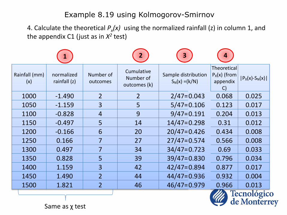
Example 8.19 using Kolmogorov-Smirnov
Rainfall (mm) (x)
normalized rainfall (z)
Number of outcomes
Cumulative Number of
outcomes (k)
Sample distribution SN(x) =(k/N)
TheoreticalPX(x) (from appendix
C)
|PX(x)-SN(x)|
1000 -1.490 2 2 2/47=0.043 0.068 0.0251050 -1.159 3 5 5/47=0.106 0.123 0.0171100 -0.828 4 9 9/47=0.191 0.204 0.0131150 -0.497 5 14 14/47=0.298 0.31 0.0121200 -0.166 6 20 20/47=0.426 0.434 0.0081250 0.166 7 27 27/47=0.574 0.566 0.0081300 0.497 7 34 34/47=0.723 0.69 0.0331350 0.828 5 39 39/47=0.830 0.796 0.0341400 1.159 3 42 42/47=0.894 0.877 0.0171450 1.490 2 44 44/47=0.936 0.932 0.0041500 1.821 2 46 46/47=0.979 0.966 0.013
Same as χ test
1 2 3
3. Calculate the simple distribution Sn(x) = k/𝑁N = number of years of data = 47
Example 8.19 using Kolmogorov-Smirnov
Rainfall (mm) (x)
normalized rainfall (z)
Number of outcomes
Cumulative Number of
outcomes (k)
Sample distribution SN(x) =(k/N)
TheoreticalPX(x) (from appendix
C)
|PX(x)-SN(x)|
1000 -1.490 2 2 2/47=0.043 0.068 0.0251050 -1.159 3 5 5/47=0.106 0.123 0.0171100 -0.828 4 9 9/47=0.191 0.204 0.0131150 -0.497 5 14 14/47=0.298 0.31 0.0121200 -0.166 6 20 20/47=0.426 0.434 0.0081250 0.166 7 27 27/47=0.574 0.566 0.0081300 0.497 7 34 34/47=0.723 0.69 0.0331350 0.828 5 39 39/47=0.830 0.796 0.0341400 1.159 3 42 42/47=0.894 0.877 0.0171450 1.490 2 44 44/47=0.936 0.932 0.0041500 1.821 2 46 46/47=0.979 0.966 0.013
Same as χ test
1 2 3 4
4. Calculate the theoretical Px(x) using the normalized rainfall (z) in column 1, and the appendix C1 (just as in X2 test)

Example 8.18 – using Kolmogorov-Smirnov
Rainfall (mm) (x)
normalized rainfall (z)
Number of outcomes
Cumulative Number of
outcomes (k)
Sample distribution SN(x) =(k/N)
TheoreticalPX(x) (from appendix
C)
|PX(x)-SN(x)|
1000 -1.490 2 2 2/47=0.043 0.068 0.0251050 -1.159 3 5 5/47=0.106 0.123 0.0171100 -0.828 4 9 9/47=0.191 0.204 0.0131150 -0.497 5 14 14/47=0.298 0.31 0.0121200 -0.166 6 20 20/47=0.426 0.434 0.0081250 0.166 7 27 27/47=0.574 0.566 0.0081300 0.497 7 34 34/47=0.723 0.69 0.0331350 0.828 5 39 39/47=0.830 0.796 0.0341400 1.159 3 42 42/47=0.894 0.877 0.0171450 1.490 2 44 44/47=0.936 0.932 0.0041500 1.821 2 46 46/47=0.979 0.966 0.013
1 2 3 4 5
6
5. Calculate |𝑃𝑥 𝑥 − 𝑆𝑁(𝑋)| = |𝑐𝑜𝑙𝑢𝑚𝑛4 − 𝑐𝑜𝑙𝑢𝑚𝑛3|
6. Determine D, which is the maximum difference between theoretical and the maximum distribution (largest value in column 5)
Example 8.18 – using Kolmogorov-Smirnov
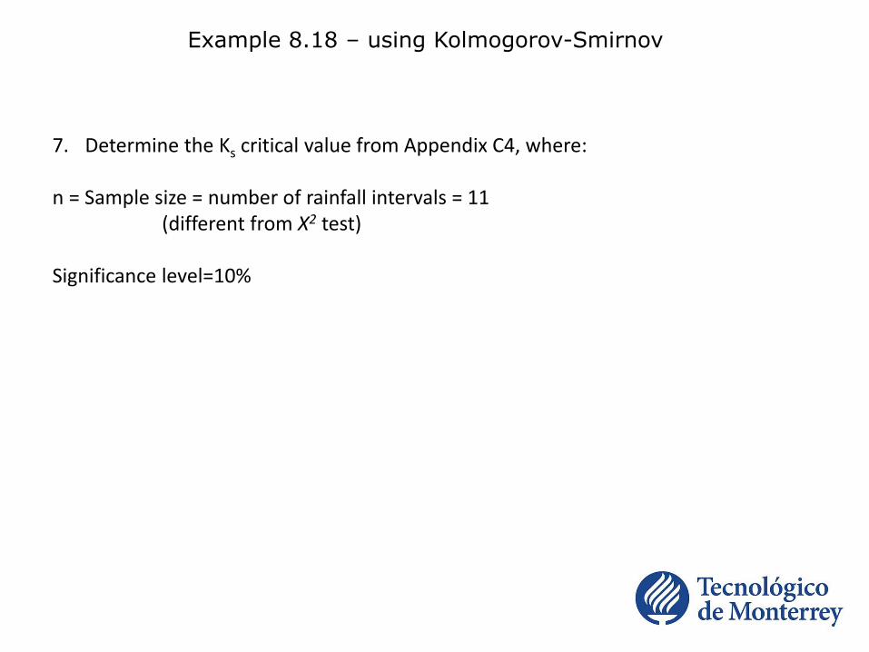
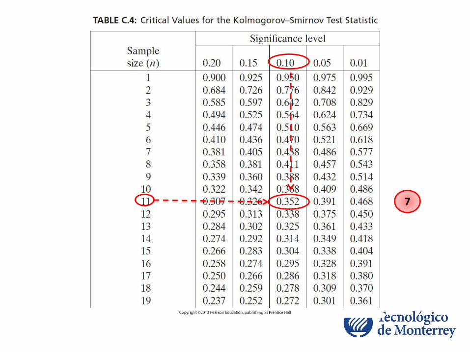
7. Determine the Ks critical value from Appendix C4, where:
n = Sample size = number of rainfall intervals = 11(different from X2 test)
Significance level=10%
7
Example 8.18 – using Kolmogorov-Smirnov
8. Determine if 𝐻0 is accepted
𝐻0 is accepted only if:
D < Ks
Since
D = 0.034 and Ks =0.352, then
𝐻0 is accepted and the data comes from normal distribution a 10% significant level
1) Do: “Flood Frequency Analysis"
MetEd Online - 3