Chapter 13 Analysis of Variance and Experimental...
35
13 - 1 Chapter 13 Analysis of Variance and Experimental Design Learning Objectives 1. Understand how the analysis of variance procedure can be used to determine if the means of more than two populations are equal. 2. Know the assumptions necessary to use the analysis of variance procedure. 3. Understand the use of the F distribution in performing the analysis of variance procedure. 4. Know how to set up an ANOVA table and interpret the entries in the table. 5. Be able to use output from computer software packages to solve analysis of variance problems. 6. Know how to use Fisher’s least significant difference (LSD) procedure and Fisher’s LSD with the Bonferroni adjustment to conduct statistical comparisons between pairs of populations means. 7. Understand the difference between a completely randomized design, a randomized block design, and factorial experiments. 8. Know the definition of the following terms: comparisonwise Type I error rate partitioning experimentwise Type I error rate blocking factor main effect level interaction treatment replication
-
Upload
nguyentram -
Category
Documents
-
view
218 -
download
0
Transcript of Chapter 13 Analysis of Variance and Experimental...

13 - 1
Chapter 13 Analysis of Variance and Experimental Design Learning Objectives 1. Understand how the analysis of variance procedure can be used to determine if the means of more
than two populations are equal. 2. Know the assumptions necessary to use the analysis of variance procedure. 3. Understand the use of the F distribution in performing the analysis of variance procedure. 4. Know how to set up an ANOVA table and interpret the entries in the table. 5. Be able to use output from computer software packages to solve analysis of variance problems. 6. Know how to use Fisher’s least significant difference (LSD) procedure and Fisher’s LSD with the
Bonferroni adjustment to conduct statistical comparisons between pairs of populations means. 7. Understand the difference between a completely randomized design, a randomized block design, and
factorial experiments. 8. Know the definition of the following terms: comparisonwise Type I error rate partitioning experimentwise Type I error rate blocking factor main effect level interaction treatment replication

Chapter 13
13 - 2
Solutions: 1. a. x = (30 + 45 + 36)/3 = 37
( )2
1
SSTRk
j jj
n x x=
= −∑ = 5(30 - 37)2 + 5(45 - 37)2 + 5(36 - 37)2 = 570
MSTR = SSTR /(k - 1) = 570/2 = 285
b. 2
1
SSE ( 1)k
j jj
n s=
= −∑ = 4(6) + 4(4) + 4(6.5) = 66
MSE = SSE /(nT - k) = 66/(15 - 3) = 5.5 c. F = MSTR /MSE = 285/5.5 = 51.82 F.05
= 3.89 (2 degrees of freedom numerator and 12 denominator) Since F = 51.82 > F.05 = 3.89, we reject the null hypothesis that the means of the three populations are
equal. d.
Source of Variation Sum of Squares Degrees of Freedom Mean Square F Treatments 570 2 285 51.82 Error 66 12 5.5 Total 636 14
2. a. x = (153 + 169 + 158)/3 = 160
( )2
1
SSTRk
j jj
n x x=
= −∑ = 4(153 - 160)2 + 4(169 - 160) 2 + 4(158 - 160) 2 = 536
MSTR = SSTR /(k - 1) = 536/2 = 268
b. 2
1
SSE ( 1)k
j jj
n s=
= −∑ = 3(96.67) + 3(97.33) +3(82.00) = 828.00
MSE = SSE /(nT - k) = 828.00 /(12 - 3) = 92.00 c. F = MSTR /MSE = 268/92 = 2.91 F.05
= 4.26 (2 degrees of freedom numerator and 9 denominator) Since F = 2.91 < F.05
= 4.26, we cannot reject the null hypothesis. d.
Source of Variation Sum of Squares Degrees of Freedom Mean Square F Treatments 536 2 268 2.91 Error 828 9 92 Total 1364 11

Analysis of Variance and Experimental Design
13 - 3
3. a. 4(100) 6(85) 5(79) 87
15x + += =
( )2
1
SSTRk
j jj
n x x=
= −∑ = 4(100 - 87) 2 + 6(85 - 87) 2 + 5(79 - 87) 2 = 1,020
MSTR = SSB /(k - 1) = 1,020/2 = 510
b. 2
1
SSE ( 1)k
j jj
n s=
= −∑ = 3(35.33) + 5(35.60) + 4(43.50) = 458
MSE = SSE /(nT - k) = 458/(15 - 3) = 38.17 c. F = MSTR /MSE = 510/38.17 = 13.36 F.05
= 3.89 (2 degrees of freedom numerator and 12 denominator) Since F = 13.36 > F.05
= 3.89 we reject the null hypothesis that the means of the three populations are equal.
d.
Source of Variation Sum of Squares Degrees of Freedom Mean Square F Treatments 1020 2 510 13.36 Error 458 12 38.17 Total 1478 14
4. a.
Source of Variation Sum of Squares Degrees of Freedom Mean Square F Treatments 1200 3 400 80 Error 300 60 5 Total 1500 63
b. F.05
= 2.76 (3 degrees of freedom numerator and 60 denominator) Since F = 80 > F.05
= 2.76 we reject the null hypothesis that the means of the 4 populations are equal. 5. a.
Source of Variation Sum of Squares Degrees of Freedom Mean Square F Treatments 120 2 60 20 Error 216 72 3 Total 336 74
b. F.05
= 3.15 (2 numerator degrees of freedom and 60 denominator) F.05
= 3.07 (2 numerator degrees of freedom and 120 denominator) The critical value is between 3.07 and 3.15
Since F = 20 must exceed the critical value, no matter what its actual value, we reject the null hypothesis that the 3 population means are equal.

Chapter 13
13 - 4
6. Manufacturer 1 Manufacturer 2 Manufacturer 3 Sample Mean 23 28 21 Sample Variance 6.67 4.67 3.33
x = (23 + 28 + 21)/3 = 24
( )2
1
SSTRk
j jj
n x x=
= −∑ = 4(23 - 24) 2 + 4(28 - 24) 2 + 4(21 - 24) 2 = 104
MSTR = SSTR /(k - 1) = 104/2 = 52
2
1
SSE ( 1)k
j jj
n s=
= −∑ = 3(6.67) + 3(4.67) + 3(3.33) = 44.01
MSE = SSE /(nT - k) = 44.01/(12 - 3) = 4.89 F = MSTR /MSE = 52/4.89 = 10.63 F.05
= 4.26 (2 degrees of freedom numerator and 9 denominator) Since F = 10.63 > F.05
= 4.26 we reject the null hypothesis that the mean time needed to mix a batch of material is the same for each manufacturer.
7.
Superior Peer Subordinate Sample Mean 5.75 5.5 5.25 Sample Variance 1.64 2.00 1.93
x = (5.75 + 5.5 + 5.25)/3 = 5.5
( )2
1
SSTRk
j jj
n x x=
= −∑ = 8(5.75 - 5.5) 2 + 8(5.5 - 5.5) 2 + 8(5.25 - 5.5) 2 = 1
MSTR = SSTR /(k - 1) = 1/2 = .5
2
1
SSE ( 1)k
j jj
n s=
= −∑ = 7(1.64) + 7(2.00) + 7(1.93) = 38.99
MSE = SSE /(nT - k) = 38.99/21 = 1.86 F = MSTR /MSE = 0.5/1.86 = 0.27 F.05
= 3.47 (2 degrees of freedom numerator and 21 denominator) Since F = 0.27 < F.05
= 3.47, we cannot reject the null hypothesis that the means of the three populations are equal; thus, the source of information does not significantly affect the dissemination of the information.
Analysis of Variance and Experimental Design
13 - 5
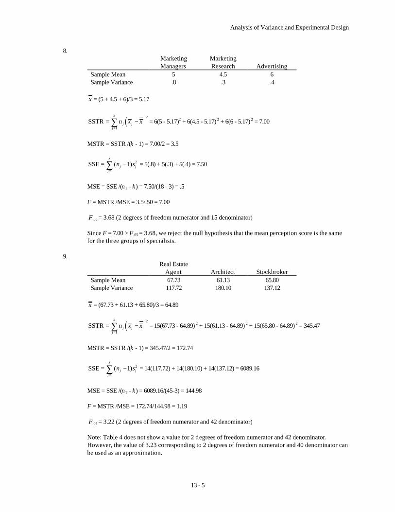
8. Marketing
Managers Marketing Research
Advertising
Sample Mean 5 4.5 6 Sample Variance .8 .3 .4
x = (5 + 4.5 + 6)/3 = 5.17
( )2
1
SSTRk
j jj
n x x=
= −∑ = 6(5 - 5.17)2 + 6(4.5 - 5.17) 2 + 6(6 - 5.17) 2 = 7.00
MSTR = SSTR /(k - 1) = 7.00/2 = 3.5
2
1
SSE ( 1)k
j jj
n s=
= −∑ = 5(.8) + 5(.3) + 5(.4) = 7.50
MSE = SSE /(nT - k) = 7.50/(18 - 3) = .5 F = MSTR /MSE = 3.5/.50 = 7.00 F.05
= 3.68 (2 degrees of freedom numerator and 15 denominator) Since F = 7.00 > F.05
= 3.68, we reject the null hypothesis that the mean perception score is the same for the three groups of specialists.
9.
Real Estate Agent
Architect
Stockbroker
Sample Mean 67.73 61.13 65.80 Sample Variance 117.72 180.10 137.12
x = (67.73 + 61.13 + 65.80)/3 = 64.89
( )2
1
SSTRk
j jj
n x x=
= −∑ = 15(67.73 - 64.89) 2 + 15(61.13 - 64.89) 2 + 15(65.80 - 64.89) 2 = 345.47
MSTR = SSTR /(k - 1) = 345.47/2 = 172.74
2
1
SSE ( 1)k
j jj
n s=
= −∑ = 14(117.72) + 14(180.10) + 14(137.12) = 6089.16
MSE = SSE /(nT - k) = 6089.16/(45-3) = 144.98 F = MSTR /MSE = 172.74/144.98 = 1.19 F.05
= 3.22 (2 degrees of freedom numerator and 42 denominator) Note: Table 4 does not show a value for 2 degrees of freedom numerator and 42 denominator.
However, the value of 3.23 corresponding to 2 degrees of freedom numerator and 40 denominator can be used as an approximation.

Chapter 13
13 - 6
Since F = 1.19 < F.05 = 3.23, we cannot reject the null hypothesis that the job stress ratings are the
same for the three occupations. 10. The Mintab output is shown below: ANALYSIS OF VARIANCE ON P/E SOURCE DF SS MS F p Industry 2 40.8 20.4 0.94 0.403 ERROR 26 563.8 21.7 TOTAL 28 604.6 INDIVIDUAL 95 PCT CI'S FOR MEAN BASED ON POOLED STDEV LEVEL N MEAN STDEV ---------+---------+---------+------- 1 12 15.250 5.463 (--------*--------) 2 7 18.286 4.071 (-----------*-----------) 3 10 16.300 3.889 (---------*---------) ---------+---------+---------+------- POOLED STDEV = 4.657 15.0 18.0 21.0 Since the p-value = 0.403 > α = 0.05, we cannot reject the null hypothesis that that the mean
price/earnings ratio is the same for these three groups of firms.
11. a / 2 .025
1 1 1 1LSD MSE 5.5 2.179 2.2 3.23
5 5i j
t tn nα
= + = + = =
1 2 30 45 15x x− = − = > LSD; significant difference
1 3 30 36 6x x− = − = > LSD; significant difference
2 3 45 36 9x x− = − = > LSD; significant difference
b. 1 2 / 21 2
1 1MSEx x tn nα
− ± +
1 2
1 1(30 45) 2.179 5.5n n
− ± +
-15 ± 3.23 = -18.23 to -11.77 12. a.
Sample 1 Sample 2 Sample 3 Sample Mean 51 77 58 Sample Variance 96.67 97.34 81.99
x = (51 + 77 + 58)/3 = 62
( )2
1
SSTRk
j jj
n x x=
= −∑ = 4(51 - 62) 2 +4(77 - 62) 2 + 4(58 - 62) 2 = 1,448

Analysis of Variance and Experimental Design
13 - 7
MSTR = SSTR /(k - 1) = 1,448/2 = 724
2
1
SSE ( 1)k
j jj
n s=
= −∑ = 3(96.67) + 3(97.34) + 3(81.99) = 828
MSE = SSE /(nT - k) = 828/(12 - 3) = 92 F = MSTR /MSE = 724/92 = 7.87 F.05
= 4.26 (2 degrees of freedom numerator and 9 denominator) Since F = 7.87 > F.05
= 4.26, we reject the null hypothesis that the means of the three populations are equal.
b. / 2 .025
1 1 1 1LSD MSE 92 2.262 46 15.34
4 4i j
t tn nα
= + = + = =
1 2 51 77 26x x− = − = > LSD; significant difference
1 3 51 58 7x x− = − = < LSD; no significant difference
2 3 77 58 19x x− = − = > LSD; significant difference
13. / 2 .0251 3
1 1 1 1LSD MSE 4.89 2.262 2.45 3.544 4
t tn nα
= + = + = =
Since 1 3 23 21 2 3.54,x x− = − = < there does not appear to be any significant difference between
the means of population 1 and population 3. 14. 1 2 LSDx x− ±
23 - 28 ± 3.54 -5 ± 3.54 = -8.54 to -1.46 15. Since there are only 3 possible pairwise comparisons we will use the Bonferroni adjustment. α = .05/3 = .017 t.017/2 = t.0085 which is approximately t.01 = 2.602
1 1 1 1
BSD 2.602 MSE 2.602 .5 1.066 6i jn n
= + = + =
1 2 5 4.5 .5x x− = − = < 1.06; no significant difference
1 3 5 6 1x x− = − = < 1.06; no significant difference

Chapter 13
13 - 8
2 3 4.5 6 1.5x x− = − = > 1.06; significant difference
16. a.
Machine 1 Machine 2 Machine 3 Machine 4 Sample Mean 7.1 9.1 9.9 11.4 Sample Variance 1.21 .93 .70 1.02
x = (7.1 + 9.1 + 9.9 + 11.4)/4 = 9.38
( )2
1
SSTRk
j jj
n x x=
= −∑ = 6(7.1 - 9.38) 2 + 6(9.1 - 9.38) 2 + 6(9.9 - 9.38) 2 + 6(11.4 - 9.38) 2 = 57.77
MSTR = SSTR /(k - 1) = 57.77/3 = 19.26
2
1
SSE ( 1)k
j jj
n s=
= −∑ = 5(1.21) + 5(.93) + 5(.70) + 5(1.02) = 19.30
MSE = SSE /(nT - k) = 19.30/(24 - 4) = .97 F = MSTR /MSE = 19.26/.97 = 19.86 F.05
= 3.10 (3 degrees of freedom numerator and 20 denominator) Since F = 19.86 > F.05
= 3.10, we reject the null hypothesis that the mean time between breakdowns is the same for the four machines.
b. Note: tα/2 is based upon 20 degrees of freedom
/ 2 .025
1 1 1 1LSD MSE 0.97 2.086 .3233 1.19
6 6i j
t tn nα
= + = + = =
2 4 9.1 11.4 2.3x x− = − = > LSD; significant difference
17. C = 6 [(1,2), (1,3), (1,4), (2,3), (2,4), (3,4)] α = .05/6 = .008 and α /2 = .004 Since the smallest value for α /2 in the t table is .005, we will use t.005 = 2.845 as an approximation for
t.004 (20 degrees of freedom)
1 1
BSD 2.845 0.97 1.626 6
= + =
Thus, if the absolute value of the difference between any two sample means exceeds 1.62, there is
sufficient evidence to reject the hypothesis that the corresponding population means are equal.
Means (1,2) (1,3) (1,4) (2,3) (2,4) (3,4) | Difference | 2 2.8 4.3 0.8 2.3 1.5 Significant ? Yes Yes Yes No Yes No

Analysis of Variance and Experimental Design
13 - 9
18. n1 = 12 n2 = 8 n3 = 10 tα/2 is based upon 27 degrees of freedom Comparing 1 and 2
.025
1 1LSD 13 2.052 2.7083 3.38
12 8t = + = =
9.95 14.75 4.8− = > LSD; significant difference
Comparing 1 and 3
1 1
LSD 2.052 13 2.052 2.3833 3.1712 10
= + = =
|9.95 - 13.5| = 3.55 > LSD; significant difference Comparing 2 and 3
1 1
LSD 2.052 13 2.052 2.9250 3.518 10
= + = =
|14.75 - 13.5| = 1.25 < LSD; no significant difference Using the Bonferroni adjustment with C = 3 α = .05 /3 = .0167 α /2 = .0083 or approximately .01 t.01= 2.473
Means (1,2) (1,3) (2,3) BSD 4.07 3.82 4.23 |Difference| 4.8 3.55 3.51 Significant ? Yes No No
Thus, using the Bonferroni adjustment, the difference between the mean price/earnings ratios of
banking firms and financial services firms is significant. 19. a. x = (156 + 142 + 134)/3 = 144
( )2
1
SSTRk
j jj
n x x=
= −∑ = 6(156 - 144) 2 + 6(142 - 144) 2 + 6(134 - 144) 2 = 1,488
b. MSTR = SSTR /(k - 1) = 1488/2 = 744 c. 2
1s = 164.4 22s = 131.2 2
3s = 110.4

Chapter 13
13 - 10
2
1
SSE ( 1)k
j jj
n s=
= −∑ = 5(164.4) + 5(131.2) +5(110.4) = 2030
d. MSE = SSE /(nT - k) = 2030/(12 - 3) = 135.3 e. F = MSTR /MSE = 744/135.3 = 5.50 F.05
= 3.68 (2 degrees of freedom numerator and 15 denominator) Since F = 5.50 > F.05
= 3.68, we reject the hypothesis that the means for the three treatments are equal. 20. a.
Source of Variation Sum of Squares Degrees of Freedom Mean Square F Treatments 1488 2 744 5.50 Error 2030 15 135.3 Total 3518 17
b. / 2
1 1 1 1LSD MSE 2.131 135.3 14.31
6 6i j
tn nα
= + = + =
|156-142| = 14 < 14.31; no significant difference |156-134| = 22 > 14.31; significant difference |142-134| = 8 < 14.31; no significant difference 21.
Source of Variation Sum of Squares Degrees of Freedom Mean Square F Treatments 300 4 75 14.07 Error 160 30 5.33 Total 460 34
22. a. H0: u1 = u2 = u3 = u4 = u5 Ha: Not all the population means are equal b. F.05
= 2.69 (4 degrees of freedom numerator and 30 denominator) Since F = 14.07 > 2.69 we reject H0
23.
Source of Variation Sum of Squares Degrees of Freedom Mean Square F Treatments 150 2 75 4.80 Error 250 16 15.63 Total 400 18
F.05
= 3.63 (2 degrees of freedom numerator and 16 denominator) Since F = 4.80 > F.05 = 3.63, we reject
the null hypothesis that the means of the three treatments are equal. 24.

Analysis of Variance and Experimental Design
13 - 11
Source of Variation Sum of Squares Degrees of Freedom Mean Square F Treatments 1200 2 600 43.99 Error 600 44 13.64 Total 1800 46
F.05
= 3.23 (2 degrees of freedom numerator and 40 denominator) F.05
= 3.15 (2 degrees of freedom numerator and 60 denominator) The critical F value is between 3.15 and 3.23. Since F = 43.99 exceeds the critical value, we reject the hypothesis that the treatment means are equal. 25.
A B C Sample Mean 119 107 100 Sample Variance 146.89 96.43 173.78
8(119) 10(107) 10(100) 107.93
28x + += =
( )2
1
SSTRk
j jj
n x x=
= −∑ = 8(119 - 107.93) 2 + 10(107 - 107.93) 2 + 10(100 - 107.93) 2 = 1617.9
MSTR = SSTR /(k - 1) = 1617.9 /2 = 809.95
2
1
SSE ( 1)k
j jj
n s=
= −∑ = 7(146.86) + 9(96.44) + 9(173.78) = 3,460
MSE = SSE /(nT - k) = 3,460 /(28 - 3) = 138.4 F = MSTR /MSE = 809.95 /138.4 = 5.85 F.05
= 3.39 (2 degrees of freedom numerator and 25 denominator) Since F = 5.85 > F.05
= 3.39, we reject the null hypothesis that the means of the three treatments are equal.
26. a.
Source of Variation Sum of Squares Degrees of Freedom Mean Square F Treatments 4560 2 2280 9.87 Error 6240 27 231.11 Total 10800 29
b. F.05
= 3.35 (2 degrees of freedom numerator and 27 denominator) Since F = 9.87 > F.05
= 3.35, we reject the null hypothesis that the means of the three assembly methods are equal.
27.
Source of Variation Sum of Squares Degrees of Freedom Mean Square F

Chapter 13
13 - 12
Between 61.64 3 20.55 17.56 Error 23.41 20 1.17 Total 85.05 23
F.05
= 3.10 (3 degrees of freedom numerator and 20 denominator) Since F = 17.56 > F.05
= 3.10, we reject the null hypothesis that the mean breaking strength of the four cables is the same.
28.
50° 60° 70° Sample Mean 33 29 28 Sample Variance 32 17.5 9.5
x = (33 + 29 + 28)/3 = 30
( )2
1
SSTRk
j jj
n x x=
= −∑ = 5(33 - 30) 2 + 5(29 - 30) 2 + 5(28 - 30) 2 = 70
MSTR = SSTR /(k - 1) = 70 /2 = 35
2
1
SSE ( 1)k
j jj
n s=
= −∑ = 4(32) + 4(17.5) + 4(9.5) = 236
MSE = SSE /(nT - k) = 236 /(15 - 3) = 19.67 F = MSTR /MSE = 35 /19.67 = 1.78 F.05
= 3.89 (2 degrees of freedom numerator and 12 denominator) Since F = 1.78 < F.05
= 3.89, we cannot reject the null hypothesis that the mean yields for the three temperatures are equal.
29.
Direct Experience
Indirect Experience
Combination
Sample Mean 17.0 20.4 25.0 Sample Variance 5.01 6.26 4.01
x = (17 + 20.4 + 25)/3 = 20.8
( )2
1
SSTRk
j jj
n x x=
= −∑ = 7(17 - 20.8) 2 + 7(20.4 - 20.8) 2 + 7(25 - 20.8) 2 = 225.68
MSTR = SSTR /(k - 1) = 225.68 /2 = 112.84
2
1
SSE ( 1)k
j jj
n s=
= −∑ = 6(5.01) + 6(6.26) + 6(4.01) = 91.68

Analysis of Variance and Experimental Design
13 - 13
MSE = SSE /(nT - k) = 91.68 /(21 - 3) = 5.09 F = MSTR /MSE = 112.84 /5.09 = 22.17 F.05
= 3.55 (2 degrees of freedom numerator and 18 denominator) Since F = 22.17 > F.05
= 3.55, we reject the null hypothesis that the means for the three groups are equal.
30.
Paint 1 Paint 2 Paint 3 Paint 4 Sample Mean 13.3 139 136 144 Sample Variance 47.5 .50 21 54.5
x = (133 + 139 + 136 + 144)/3 = 138
( )2
1
SSTRk
j jj
n x x=
= −∑ = 5(133 - 138) 2 + 5(139 - 138) 2 + 5(136 - 138) 2 + 5(144 - 138) 2 = 330
MSTR = SSTR /(k - 1) = 330 /3 = 110
2
1
SSE ( 1)k
j jj
n s=
= −∑ = 4(47.5) + 4(50) + 4(21) + 4(54.5) = 692
MSE = SSE /(nT - k) = 692 /(20 - 4) = 43.25 F = MSTR /MSE = 110 /43.25 = 2.54 F.05
= 3.24 (3 degrees of freedom numerator and 16 denominator) Since F = 2.54 < F.05
= 3.24, we cannot reject the null hypothesis that the mean drying times for the four paints are equal.
31.
A B C Sample Mean 20 21 25 Sample Variance 1 25 2.5
x = (20 + 21 + 25)/3 = 22
( )2
1
SSTRk
j jj
n x x=
= −∑ = 5(20 - 22) 2 + 5(21 - 22) 2 + 5(25 - 22) 2 = 70
MSTR = SSTR /(k - 1) = 70 /2 = 35
2
1
SSE ( 1)k
j jj
n s=
= −∑ = 4(1) + 4(2.5) + 4(2.5) = 24
MSE = SSE /(nT - k) = 24 /(15 - 3) = 2

Chapter 13
13 - 14
F = MSTR /MSE = 35 /2 = 17.5 F.05
= 3.89 (2 degrees of freedom numerator and 12 denominator) Since F = 17.5 > F.05
= 3.89, we reject the null hypothesis that the mean miles per gallon ratings are the same for the three automobiles.
32. Note: degrees of freedom for tα/2 are 18
/ 2 .025
1 1 1 1LSD MSE 5.09 2.101 1.4543 2.53
7 7i j
t tn nα
= + = + = =
1 2 17.0 20.4 3.4x x− = − = > 2.53; significant difference
1 3 17.0 25.0 8x x− = − = > 2.53; significant difference
2 3 20.4 25 4.6x x− = − = >2.53; significant difference
33. Note: degrees of freedom for tα/2 are 12
/ 2 .025
1 1 1 1LSD MSE 2 2.179 .8 1.95
5 5i j
t tn nα
= + = + = =
1 2 20 21 1x x− = − = < 1.95; no significant difference
1 3 20 25 5x x− = − = > 1.95; significant difference
2 3 21 25 4x x− = − = > 1.95; significant difference
34. Treatment Means: 1xg = 13.6 2xg = 11.0 3xg = 10.6
Block Means: 1x g= 9 2x g = 7.67 3x g = 15.67 4x g = 18.67 5x g = 7.67
Overall Mean: x = 176/15 = 11.73
Step 1
( )2SST ij
i j
x x= −∑∑ = (10 - 11.73) 2 + (9 - 11.73) 2 + · · · + (8 - 11.73) 2 = 354.93

Analysis of Variance and Experimental Design
13 - 15
Step 2
( )2SSTR j
j
b x x= −∑ g = 5 [ (13.6 - 11.73) 2 + (11.0 - 11.73) 2 + (10.6 - 11.73) 2 ] = 26.53
Step 3
( )2SSBL i
i
k x x= −∑ g = 3 [ (9 - 11.73) 2 + (7.67 - 11.73) 2 + (15.67 - 11.73) 2 +
(18.67 - 11.73) 2 + (7.67 - 11.73) 2 ] = 312.32 Step 4 SSE = SST - SSTR - SSBL = 354.93 - 26.53 - 312.32 = 16.08
Source of Variation Sum of Squares Degrees of Freedom Mean Square F Treatments 26.53 2 13.27 6.60 Blocks 312.32 4 78.08 Error 16.08 8 2.01 Total 354.93 14
F.05
= 4.46 (2 degrees of freedom numerator and 8 denominator) Since F = 6.60 > F.05
= 4.46, we reject the null hypothesis that the means of the three treatments are equal.
35.
Source of Variation Sum of Squares Degrees of Freedom Mean Square F Treatments 310 4 77.5 17.69 Blocks 85 2 42.5 Error 35 8 4.38 Total 430 14
F.05
= 3.84 (4 degrees of freedom numerator and 8 denominator) Since F = 17.69 > F.05
= 3.84, we reject the null hypothesis that the means of the treatments are equal. 36.
Source of Variation Sum of Squares Degrees of Freedom Mean Square F Treatments 900 3 300 12.60 Blocks 400 7 57.14 Error 500 21 23.81 Total 1800 31
F.05
= 3.07 (3 degrees of freedom numerator and 21 denominator) Since F = 12.60 > F.05
= 3.07, we reject the null hypothesis that the means of the treatments are equal. 37. Treatment Means: 1xg = 56 2xg = 44

Chapter 13
13 - 16
Block Means: 1x g= 46 2x g = 49.5 3x g = 54.5
Overall Mean: x = 300/6 = 50 Step 1
( )2SST ij
i j
x x= −∑∑ = (50 - 50) 2 + (42 - 50) 2 + · · · + (46 - 50) 2 = 310
Step 2
( )2SSTR j
j
b x x= −∑ g = 3 [ (56 - 50) 2 + (44 - 50) 2 ] = 216
Step 3
( )2SSBL i
i
k x x= −∑ g = 2 [ (46 - 50) 2 + (49.5 - 50) 2 + (54.5 - 50) 2 ] = 73
Step 4 SSE = SST - SSTR - SSBL = 310 - 216 - 73 = 21
Source of Variation Sum of Squares Degrees of Freedom Mean Square F Treatments 216 1 216 20.57 Blocks 73 2 36.5 Error 21 2 10.5 Total 310 5
F.05
= 18.51 (1 degree of freedom numerator and 2 denominator) Since F = 20.57 > F.05
= 18.51, we reject the null hypothesis that the mean tuneup times are the same for both analyzers.
38.
Source of Variation Sum of Squares Degrees of Freedom Mean Square F Treatments 45 4 11.25 7.12 Blocks 36 3 12 Error 19 12 1.58 Total 100 19
F.05 = 3.26 (4 degrees of freedom numerator and 12 denominator)
Since F = 7.12 > F.05
= 3.26, we reject the null hypothesis that the mean total audit times for the five auditing procedures are equal.
39. Treatment Means:

Analysis of Variance and Experimental Design
13 - 17
1xg = 16 2xg = 15 3xg = 21
Block Means: 1x g= 18.67 2x g = 19.33 3x g = 15.33 4x g = 14.33 5x g = 19
Overall Mean: x = 260/15 = 17.33 Step 1
( )2SST ij
i j
x x= −∑∑ = (16 - 17.33) 2 + (16 - 17.33) 2 + · · · + (22 - 17.33) 2 = 175.33
Step 2
( )2SSTR j
j
b x x= −∑ g = 5 [ (16 - 17.33) 2 + (15 - 17.33) 2 + (21 - 17.33) 2 ] = 103.33
Step 3
( )2SSBL i
i
k x x= −∑ g = 3 [ (18.67 - 17.33) 2 + (19.33 - 17.33) 2 + · · · + (19 - 17.33) 2 ] = 64.75
Step 4 SSE = SST - SSTR - SSBL = 175.33 - 103.33 - 64.75 = 7.25
Source of Variation Sum of Squares Degrees of Freedom Mean Square F Treatments 100.33 2 51.67 56.78 Blocks 64.75 4 16.19 Error 7.25 8 .91 Total 175.33 14
F.05
= 4.46 (2 degrees of freedom numerator and 8 denominator) Since F = 56.78 > F.05
= 4.46, we reject the null hypothesis that the mean times for the three systems are equal.
40. The Minitab output for these data is shown below: ANALYSIS OF VARIANCE BPM SOURCE DF SS MS Block 9 2796 311 Treat 3 19805 6602

Chapter 13
13 - 18
ERROR 27 7949 294 TOTAL 39 30550 Individual 95% CI Treat Mean ----+---------+---------+---------+------- 1 178.0 (-----*-----) 2 171.0 (-----*----) 3 175.0 (-----*----) 4 123.6 (-----*----) ----+---------+---------+---------+------- 120.0 140.0 160.0 180.0 F.05
= 2.96 (3 degrees of freedom numerator and 27 denominator) Since F = 6602 /294 = 22.46 > 2.96, we reject the null hypotheses that the mean heart rate for the four
methods are equal. 41.
Factor A
Level 2
Factor B Means
11x = 150
Level 1 Level 2 Level 3 Means
Factor B Factor A
Level 1 12x = 78 13x = 84 1x g = 104
21x = 110
1xg = 130
22x = 116
2xg = 97
23x = 128
3xg = 106
2x g = 118
x = 111
Step 1
( )2SST ijk
i j k
x x= −∑∑∑ = (135 - 111) 2 + (165 - 111) 2 + · · · + (136 - 111) 2 = 9,028
Step 2
( )2SSA j
i
br x x= −∑ g = 3 (2) [ (104 - 111) 2 + (118 - 111) 2 ] = 588
Step 3
( )2SSB j
j
ar x x= −∑ g = 2 (2) [ (130 - 111) 2 + (97 - 111) 2 + (106 - 111) 2 ] = 2,328
Step 4
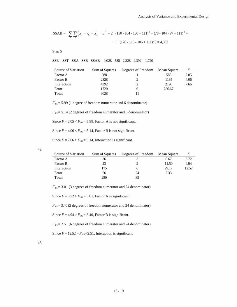
Analysis of Variance and Experimental Design
13 - 19
( )2SSAB i j i j
i j
r x x x x= − − +∑∑ g g = 2 [ (150 - 104 - 130 + 111) 2 + (78 - 104 - 97 + 111) 2 +
· · · + (128 - 118 - 106 + 111) 2 ] = 4,392 Step 5 SSE = SST - SSA - SSB - SSAB = 9,028 - 588 - 2,328 - 4,392 = 1,720
Source of Variation Sum of Squares Degrees of Freedom Mean Square F Factor A 588 1 588 2.05 Factor B 2328 2 1164 4.06 Interaction 4392 2 2196 7.66 Error 1720 6 286.67 Total 9028 11
F.05
= 5.99 (1 degree of freedom numerator and 6 denominator) F.05
= 5.14 (2 degrees of freedom numerator and 6 denominator) Since F = 2.05 < F.05
= 5.99, Factor A is not significant. Since F = 4.06 < F.05
= 5.14, Factor B is not significant. Since F = 7.66 > F.05
= 5.14, Interaction is significant. 42.
Source of Variation Sum of Squares Degrees of Freedom Mean Square F Factor A 26 3 8.67 3.72 Factor B 23 2 11.50 4.94 Interaction 175 6 29.17 12.52 Error 56 24 2.33 Total 280 35
F.05
= 3.01 (3 degrees of freedom numerator and 24 denominator) Since F = 3.72 > F.05
= 3.01, Factor A is significant. F.05
= 3.40 (2 degrees of freedom numerator and 24 denominator) Since F = 4.94 > F.05
= 3.40, Factor B is significant. F.05
= 2.51 (6 degrees of freedom numerator and 24 denominator) Since F = 12.52 > F.05
=2.51, Interaction is significant 43.

Chapter 13
13 - 20
Factor A B
Factor B Means
11x = 10
Small Large Means
Factor B Factor B
12x = 10 1x g = 10
21x = 18
1xg = 14
22x = 28
2xg = 18
2x g = 23
x = 16
A
C31x = 14 32x = 16 3x g = 15
Step 1
( )2SST ijk
i j k
x x= −∑∑∑ = (8 - 16) 2 + (12 - 16) 2 + (12 - 16) 2 + · · · + (14 - 16) 2 = 544
Step 2
( )2SSA i
i
br x x= −∑ g = 2 (2) [ (10- 16) 2 + (23 - 16) 2 + (15 - 16) 2 ] = 344
Step 3
( )2SSB j
j
ar x x= −∑ g = 3 (2) [ (14 - 16) 2 + (18 - 16) 2 ] = 48
Step 4
( )2SSAB i j i j
i j
r x x x x= − − +∑∑ g g = 2 [ (10 - 10 - 14 + 16) 2 + · · · + (16 - 15 - 18 +16) 2 ] = 56
Step 5 SSE = SST - SSA - SSB - SSAB = 544 - 344 - 48 - 56 = 96
Source of Variation Sum of Squares Degrees of Freedom Mean Square F Factor A 344 2 172 172/16 = 10.75 Factor B 48 1 48 48/16 = 3.00 Interaction 56 2 28 28/16 = 1.75 Error 96 6 16 Total 544 11
F.05
= 5.14 (2 degrees of freedom numerator and 6 denominator) Since F = 10.75 > F.05
= 5.14, Factor A is significant, there is a difference due to the type of advertisement design.

Analysis of Variance and Experimental Design
13 - 21
F.05
= 5.99 (1 degree of freedom numerator and 6 denominator) Since F = 3 < F.05
= 5.99, Factor B is not significant; there is not a significant difference due to size of advertisement.
Since F = 1.75 < F.05
= 5.14, Interaction is not significant. 44.
Factor A
Method 2
Factor B Means
11x = 42
RollerCoaster
ScreamingDemon
LogFlume Means
Factor B Factor A
Method 112x = 48 13x = 48 1x g = 46
21x = 50
1xg = 46
22x = 48
2xg = 48
23x = 46
3xg = 47
2x g = 48
x = 47
Step 1
( )2SST ijk
i j k
x x= −∑∑∑ = (41 - 47) 2 + (43 - 47) 2 + · · · + (44 - 47) 2 = 136
Step 2
( )2SSA i
i
br x x= −∑ g = 3 (2) [ (46 - 47) 2 + (48 - 47) 2 ] = 12
Step 3
( )2SSB j
j
ar x x= −∑ g = 2 (2) [ (46 - 47) 2 + (48 - 47) 2 + (47 - 47) 2 ] = 8
Step 4
( )2SSAB i j i j
i j
r x x x x= − − +∑∑ g g = 2 [ (41 - 46 - 46 + 47) 2 + · · · + (44 - 48 - 47 + 47) 2 ] = 56
Step 5 SSE = SST - SSA - SSB - SSAB = 136 - 12 - 8 - 56 = 60
Source of Variation Sum of Squares Degrees of Freedom Mean Square F
Chapter 13
13 - 22
Factor A 12 1 12 12/10 = 1.2 Factor B 8 2 4 4/10 = .4 Interaction 56 2 28 28/10 = 2.8 Error 60 6 10 Total 136 11
F.05
= 5.99 (1 numerator degree of freedom and 6 denominator) F.05
= 5.14 (2 numerator degrees of freedom and 6 denominator) Since none of the F values exceed the corresponding critical values, there is no significant effect due
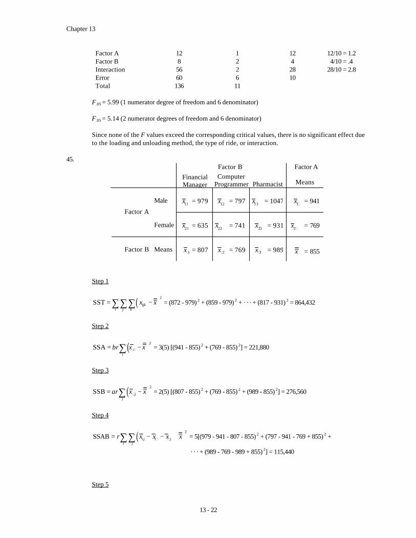
to the loading and unloading method, the type of ride, or interaction. 45.
Factor A
Female
Factor B Means
11x = 979
FinancialManager
ComputerProgrammer Pharmacist Means
Factor B Factor A
Male12x = 797 13x = 1047 1x g = 941
21x = 635
1xg = 807
22x = 741
2xg = 769
23x = 931
3xg = 989
2x g = 769
x = 855
Step 1
( )2SST ijk
i j k
x x= −∑∑∑ = (872 - 979) 2 + (859 - 979) 2 + · · · + (817 - 931) 2 = 864,432
Step 2
( )2SSA i
i
br x x= −∑ g = 3(5) [(941 - 855) 2 + (769 - 855) 2] = 221,880
Step 3
( )2SSB j
j
ar x x= −∑ g = 2(5) [(807 - 855) 2 + (769 - 855) 2 + (989 - 855) 2] = 276,560
Step 4
( )2SSAB i j i j
i j
r x x x x= − − +∑∑ g g = 5[(979 - 941 - 807 - 855) 2 + (797 - 941 - 769 + 855) 2 +
· · · + (989 - 769 - 989 + 855) 2] = 115,440 Step 5

Analysis of Variance and Experimental Design
13 - 23
SSE = SST - SSA - SSB - SSAB = 864,432 - 221,880 - 276,560 - 115,440 = 250,552
Source of Variation Sum of Squares Degrees of Freedom Mean Square F Factor A 221,880 1 221,880 21.25 Factor B 276,560 2 138,280 13.25 Interaction 115,440 2 57,720 5.53 Error 250,552 24 10,440 Total 864,432 29
F.05
= 4.26 (1 degree of freedom numerator and 24 denominator) F.05
= 3.40 (2 degrees of freedom numerator and 24 denominator) Since F = 21.25 > F.05
= 4.26, Factor A (gender) is not significant. Since F = 13.25 > F.05
= 3.40, Factor B (occupation) is significant. Since F = 5.53 > F.05
= 3.40, Interaction is significant. 46. 1x g= (1.13 + 1.56 + 2.00)/3 = 1.563
2x g = (0.48 + 1.68 + 2.86)/3 = 1.673
1xg = (1.13 + 0.48)/2 = 0.805
2xg = (1.56 + 1.68)/2 = 1.620
3xg = (2.00 + 2.86)/2 = 2.43
x = (1.13 + 1.56 + 2.00 + 0.48 + 1.68 + 2.86)/6 = 1.618 Step 1 SST = 327.50 (given in problem statement) Step 2
( )2SSA i
i
br x x= −∑ g = 3(25)[(1.563 - 1.618)2 + (1.673 - 1.618)2] = 0.4538
Step 3
( )2SSB j
j
ar x x= −∑ g = 2(25)[(0.805 - 1.618)2 + (1.62 - 1.618) 2 + (2.43 - 1.618) 2] = 66.0159
Step 4

Chapter 13
13 - 24
( )2SSAB i j i j
i j
r x x x x= − − +∑∑ g g = 25[(1.13 - 1.563 - 0.805 + 1.618) 2 + (1.56 - 1.563 - 1.62
+ 1.618) 2 + · · · + (2.86 - 1.673 - 2.43 + 1.618) 2] = 14.2525 Step 5 SSE = SST - SSA - SSB - SSAB = 327.50 - 0.4538 - 66.0159 - 14.2525
Source of Variation Sum of Squares Degrees of Freedom Mean Square F Factor A 0.4538 1 0.4538 0.2648 Factor B 66.1059 2 33.0080 19.2608 Interaction 14.2525 2 7.1263 4.1583 Error 246.7778 144 1.7137 Total 327.5000 149
F.05
for 1 degree of freedom numerator and 144 degrees of freedom denominator is between 3.92 and 3.84.
F.05
for 2 degrees of freedom numerator and 144 denominator is between 3.07 and 3.00. Since 0.2648 < F.05
= 3.84, Factor A is not significant Since 19.2608 > F.05
= 3.07, Factor B is significant Since 4.1583 > F.05
= 3.07, Interaction is significant 47. a.
Area 1 Area 2 Sample Mean 96 94 Sample Variance 50 40
pooled estimate =2 2
1 2 50 4045
2 2s s+ +
= =
estimate of standard deviation of 1 2
1 145 4.74
4 4x x − = + =
1 2 96 94 .424.74 4.74
x xt − −= = =
t.025 = 2.447 (6 degrees of freedom) Since t = .42 < t.025 = 2.477, the means are not significantly different. b. x = (96 + 94)/2 = 95
( )2
1
SSTRk
j jj
n x x=
= −∑ = 4(96 - 95) 2 + 4(94 - 95) 2 = 8
MSTR = SSTR /(k - 1) = 8 /1 = 8

Analysis of Variance and Experimental Design
13 - 25
2
1
SSE ( 1)k
j jj
n s=
= −∑ = 3(50) + 3(40) = 270
MSE = SSE /(nT - k) = 270 /(8 - 2) = 45 F = MSTR /MSE = 8 /45 = .18 F.05
= 5.99 (1 degree of freedom numerator and 6 denominator) Since F = .18 < F.05
= 5.99 the means are not significantly different. c.
Area 1 Area 2 Area 3 Sample Mean 96 94 83 Sample Variance 50 40 42
x = (96 + 94 + 83)/3 = 91
( )2
1
SSTRk
j jj
n x x=
= −∑ = 4(96 - 91) 2 + 4(94 - 91) 2 + 4(83 - 91) 2 = 392
MSTR = SSTR /(k - 1) = 392 /2 = 196
2
1
SSE ( 1)k
j jj
n s=
= −∑ = 3(50) + 3(40) + 3(42) = 396
MSTR = SSE /(nT - k) = 396 /(12 - 3) = 44 F = MSTR /MSE = 196 /44 = 4.45 F.05
= 4.26 (2 degrees of freedom numerator and 6 denominator) Since F = 4.45 > F.05
= 4.26 we reject the null hypothesis that the mean asking prices for all three areas are equal.
48. The Minitab output for these data is shown below: Analysis of Variance Source DF SS MS F P Factor 2 753.3 376.6 18.59 0.000 Error 27 546.9 20.3 Total 29 1300.2 Individual 95% CIs For Mean Based on Pooled StDev Level N Mean StDev ---------+---------+---------+------- SUV 10 58.600 4.575 (-----*-----) Small 10 48.800 4.211 (-----*----) FullSize 10 60.100 4.701 (-----*-----) ---------+---------+---------+------- Pooled StDev = 4.501 50.0 55.0 60.0

Chapter 13
13 - 26
Because the p-value = .000 < α = .05, we can reject the null hypothesis that the mean resale value is the same. It appears that the mean resale value for small pickup trucks is much smaller than the mean resale value for sport utility vehicles or full-size pickup trucks.
49.
Food Personal Care Retail Sample Mean 52.25 62.25 55.75 Sample Variance 22.25 15.58 4.92
x = (52.25 + 62.25 + 55.75)/3 = 56.75
( )2
1
SSTRk
j jj
n x x=
= −∑ = 4(52.25 - 56.75) 2 + 4(62.25 - 56.75) 2 + 4(55.75 - 56.75) 2 = 206
MSTR = SSTR /(k - 1) = 206 /2 = 103
2
1
SSE ( 1)k
j jj
n s=
= −∑ = 3(22.25) + 3(15.58) + 3(4.92) = 128.25
MSE = SSE /(nT - k) = 128.25 /(12 - 3) = 14.25 F = MSTR /MSE = 103 /14.25 = 7.23 F.05
= 4.26 (2 degrees of freedom numerator and 9 denominator) Since F = 7.23 exceeds the critical F value, we reject the null hypothesis that the mean age of
executives is the same in the three categories of companies. 50.
Lawyer
Physical Therapist
Cabinet Maker
Systems Analyst
Sample Mean 50.0 63.7 69.1 61.2 Sample Variance 124.22 164.68 105.88 136.62
50.0 63.7 69.1 61.2
614
x+ + +
= =
( )2
1
SSTRk
j jj
n x x=
= −∑ = 10(50.0 - 61) 2 + 10(63.7 - 61) 2 + 10(69.1 - 61) 2 + 10(61.2 - 61) 2 = 1939.4
MSTR = SSTR /(k - 1) = 1939.4 /3 = 646.47
2
1
SSE ( 1)k
j jj
n s=
= −∑ = 9(124.22) + 9(164.68) + 9(105.88) + 9(136.62) = 4,782.60
MSE = SSE /(nT - k) = 4782.6 /(40 - 4) = 132.85 F = MSTR /MSE = 646.47 /132.85 = 4.87 F.05
= 2.84 (3 degrees of numerator and 40 denominator)

Analysis of Variance and Experimental Design
13 - 27
F.05 = 2.76 (3 degrees of freedom numerator and 60 denominator)
Thus, the critical F value is between 2.76 and 2.84. Since F = 4.87 exceeds the critical F value, we reject the null hypothesis that the mean job satisfaction
rating is the same for the four professions. 51. The Minitab output for these data is shown below: Analysis of Variance Source DF SS MS F P Factor 2 4339 2169 3.66 0.039 Error 27 15991 592 Total 29 20330 Individual 95% CIs For Mean Based on Pooled StDev Level N Mean StDev ---+---------+---------+---------+--- West 10 108.00 23.78 (-------*-------) South 10 91.70 19.62 (-------*-------) NE 10 121.10 28.75 (-------*------) ---+---------+---------+---------+--- Pooled StDev = 24.34 80 100 120 140
Because the p-value = .039 < α = .05, we can reject the null hypothesis that the mean rate for the three
regions is the same. 52. The Mintab output is shown below: ANALYSIS OF VARIANCE SOURCE DF SS MS F p FACTOR 3 1271.0 423.7 8.74 0.000 ERROR 36 1744.2 48.4 TOTAL 39 3015.2 INDIVIDUAL 95 PCT CI'S FOR MEAN BASED ON POOLED STDEV LEVEL N MEAN STDEV --+---------+---------+---------+---- West 10 60.000 7.218 (------*-----) South 10 45.400 7.610 (------*-----) N.Cent 10 47.300 6.778 (------*-----) N.East 10 52.100 6.152 (-----*------) --+---------+---------+---------+---- POOLED STDEV = 6.961 42.0 49.0 56.0 63.0 Since the p-value = 0.000 < α = 0.05, we can reject the null hypothesis that that the mean base salary
for art directors is the same for each of the four regions.

Chapter 13
13 - 28
53. The Minitab output for these data is shown below: Analysis of Variance Source DF SS MS F P Factor 2 12.402 6.201 9.33 0.001 Error 37 24.596 0.665 Total 39 36.998 Individual 95% CIs For Mean Based on Pooled StDev Level N Mean StDev ------+---------+---------+---------+ Receiver 15 7.4133 0.8855 (-------*------) Guard 13 6.1077 0.7399 (-------*------) Tackle 12 7.0583 0.8005 (-------*-------) ------+---------+---------+---------+ Pooled StDev = 0.8153 6.00 6.60 7.20 7.80
Because the p-value = .001 < α = .05, we can reject the null hypothesis that the mean rating for the three positions is the same. It appears that wide receivers and tackles have a higher mean rating than guards.
54.
X Y Z Sample Mean 92 97 84 Sample Variance 30 6 35.33
x = (92 + 97 + 44) /3 = 91
( )2
1
SSTRk
j jj
n x x=
= −∑ = 4(92 - 91) 2 + 4(97 - 91) 2 + 4(84 - 91) 2 = 344
MSTR = SSTR /(k - 1) = 344 /2 = 172
2
1
SSE ( 1)k
j jj
n s=
= −∑ = 3(30) + 3(6) + 3(35.33) = 213.99
MSE = SSE /(nT - k) = 213.99 /(12 - 3) = 23.78 F = MSTR /MSE = 172 /23.78 = 7.23 F.05
= 4.26 (2 degrees of freedom numerator and 9 denominator) Since F = 7.23 > F.05
= 4.26, we reject the null hypothesis that the mean absorbency ratings for the three brands are equal.
55.
First Year Second Year Third Year Fourth Year Sample Mean 1.03 -0.99 15.24 9.81 Sample Variance 416.93 343.04 159.31 55.43
x = (1.03 - .99 + 15.24 + 9.81) /4 = 6.27

Analysis of Variance and Experimental Design
13 - 29
( )2
1
SSTRk
j jj
n x x=
= −∑ = 7(1.03 - 6.27) 2 + 7(-.99 - 6.27) 2 + 7(15.24 - 6.27) 2 + (9.81 - 6.27) 2
= 1,212.10 MSTR = SSTR /(k - 1) = 1,212.10 /3 = 404.03
2
1
SSE ( 1)k
j jj
n s=
= −∑ = 6(416.93) + 6(343.04) + 6(159.31) + 6(55.43) = 5,848.26
MSE = SSE /(nT - k) = 5,848.26 /(28 - 4) = 243.68 F = MSTR /MSE = 404.03 /243.68 = 1.66 F.05
= 3.01 (3 degrees of freedom numerator and 24 denominator) Since F = 1.66 < F.05
= 3.01, we can not reject the null hypothesis that the mean percent changes in each of the four years are equal.
56.
Method A Method B Method C Sample Mean 90 84 81 Sample Variance 98.00 168.44 159.78
x = (90 + 84 + 81) /3 = 85
( )2
1
SSTRk
j jj
n x x=
= −∑ = 10(90 - 85) 2 + 10(84 - 85) 2 + 10(81 - 85) 2 = 420
MSTR = SSTR /(k - 1) = 420 /2 = 210
2
1
SSE ( 1)k
j jj
n s=
= −∑ = 9(98.00) + 9(168.44) + 9(159.78) = 3,836
MSE = SSE /(nT - k) = 3,836 /(30 - 3) = 142.07 F = MSTR /MSE = 210 /142.07 = 1.48 F.05
= 3.35 (2 degrees of freedom numerator and 27 denominator) Since F = 1.48 < F.05
= 3.35, we can not reject the null hypothesis that the means are equal. 57.
Type A Type B Type C Type D Sample Mean 32,000 27,500 34,200 30,300 Sample Variance 2,102,500 2,325,625 2,722,500 1,960,000
x = (32,000 + 27,500 + 34,200 + 30,000) /4 = 31,000

Chapter 13
13 - 30
( )2
1
SSTRk
j jj
n x x=
= −∑ = 30(32,000 - 31,000) 2 + 30(27,500 - 31,000) 2 + 30(34,200 - 31,000) 2 +
30(30,300 - 31,000) 2 = 719,400,000 MSTR = SSTR /(k - 1) = 719,400,000 /3 = 239,800,000
2
1
SSE ( 1)k
j jj
n s=
= −∑ = 29(2,102,500) + 29(2,325,625) + 29(2,722,500) + 29(1,960,000)
= 264,208,125 MSE = SSE /(nT - k) = 264,208,125 /(120 - 4) = 2,277,656.25 F = MSTR /MSE = 239,800,000 /2,277,656.25 = 105.28 F.05
is approximately 2.68, the table value for 3 degrees of freedom numerator and 120 denominator; the value we would look up, if it were available, would correspond to 116 denominator degrees of freedom. Since F = 105.28 exceeds F.05, whatever its value actually is, we reject the null hypothesis that the population means are equal.
58.
Design A Design B Design C Sample Mean 90 107 109 Sample Variance 82.67 68.67 100.67
x = (90 + 107 + 109) /3 = 102
( )2
1
SSTRk
j jj
n x x=
= −∑ = 4(90 - 102) 2 +4(107 - 102) 2 +(109 - 102) 2 = 872
MSTR = SSTR /(k - 1) = 872 /2 = 436
2
1
SSE ( 1)k
j jj
n s=
= −∑ = 3(82.67) + 3(68.67) + 3(100.67) = 756.03
MSE = SSE /(nT - k) = 756.03 /(12 - 3) = 84 F = MSTR /MSE = 436 /84 = 5.19 F.05
= 4.26 (2 degrees of freedom numerator and 9 denominator) Since F = 5.19 > F.05
= 4.26, we reject the null hypothesis that the mean lifetime in hours is the same for the three designs.
59. a.
Nonbrowser Light Browser Heavy Browser Sample Mean 4.25 5.25 5.75 Sample Variance 1.07 1.07 1.36
x = (4.25 + 5.25 + 5.75) /3 = 5.08

Analysis of Variance and Experimental Design
13 - 31
( )2
1
SSTRk
j jj
n x x=
= −∑ = 8(4.25 - 5.08) 2 + 8(5.25 - 5.08) 2 + 8(5.75 - 5.08) 2 = 9.33
MSB = SSB /(k - 1) = 9.33 /2 = 4.67
2
1
SSW ( 1)k
j jj
n s=
= −∑ = 7(1.07) + 7(1.07) + 7(1.36) = 24.5
MSW = SSW /(nT - k) = 24.5 /(24 - 3) = 1.17 F = MSB /MSW = 4.67 /1.17 = 3.99 F.05
= 3.47 (2 degrees of freedom numerator and 21 denominator) Since F = 3.99 > F.05
= 3.47, we reject the null hypothesis that the mean comfort scores are the same for the three groups.
b. / 2
1 1 1 1LSD MSW 2.080 1.17 1.12
8 8i j
tn nα
= + = + =
Since the absolute value of the difference between the sample means for nonbrowsers and light browsers is 4.25 5.25 1− = , we cannot reject the null hypothesis that the two population means are
equal. 60. Treatment Means: 1x⋅ = 22.8 2x⋅ = 24.8 3x⋅ = 25.80
Block Means: 1x ⋅ = 19.67 2x ⋅ = 25.67 3x ⋅ = 31 4x ⋅ = 23.67 5x ⋅ = 22.33
Overall Mean: x = 367 /15 = 24.47 Step 1
( )2SST ij
i j
x x= −∑∑ = (18 - 24.47) 2 + (21 - 24.47) 2 + · · · + (24 - 24.47) 2 = 253.73
Step 2
( )2SSTR j
j
b x x= −∑ g = 5 [ (22.8 - 24.47) 2 + (24.8 - 24.47) 2 + (25.8 - 24.47) 2 ] = 23.33

Chapter 13
13 - 32
Step 3
( )2SSBL i
i
k x x= −∑ g = 3 [ (19.67 - 24.47) 2 + (25.67 - 24.47) 2 + · · · + (22.33 - 24.47) 2 ] = 217.02
Step 4 SSE = SST - SSTR - SSBL = 253.73 - 23.33 - 217.02 = 13.38
Source of Variation Sum of Squares Degrees of Freedom Mean Square F Treatment 23.33 2 11.67 6.99 Blocks 217.02 4 54.26 32.49 Error 13.38 8 1.67 Total 253.73 14
F.05
= 4.46 (2 degrees of freedom numerator and 8 denominator) Since F = 6.99 > F.05
= 4.46 we reject the null hypothesis that the mean miles per gallon ratings for the three brands of gasoline are equal.
61.
I II III Sample Mean 22.8 24.8 25.8 Sample Variance 21.2 9.2 27.2
x = (22.8 + 24.8 + 25.8) /3 = 24.47
( )2
1
SSTRk
j jj
n x x=
= −∑ = 5(22.8 - 24.47) 2 + 5(24.8 - 24.47) 2 + 5(25.8 - 24.47) 2 = 23.33
MSTR = SSTR /(k - 1) = 23.33 /2 = 11.67
2
1
SSE ( 1)k
j jj
n s=
= −∑ = 4(21.2) + 4(9.2) + 4(27.2) = 230.4
MSE = SSE /(nT - k) = 230.4 /(15 - 3) = 19.2 F = MSTR /MSE = 11.67 /19.2 = .61 F.05
= 3.89 (2 degrees of freedom numerator and 12 denominator) Since F = .61 < F.05
= 3.89, we cannot reject the null hypothesis that the mean miles per gallon ratings for the three brands of gasoline are equal.
Thus, we must remove the block effect in order to detect a significant difference due to the brand of
gasoline. The following table illustrates the relationship between the randomized block design and the completely randomized design.

Analysis of Variance and Experimental Design
13 - 33
Sum of Squares
Randomized Block Design
Completely Randomized Design
SST 253.73 253.73 SSTR 23.33 23.33 SSBL 217.02 does not exist SSE 13.38 230.4
Note that SSE for the completely randomized design is the sum of SSBL (217.02) and SSE (13.38) for
the randomized block design. This illustrates that the effect of blocking is to remove the block effect from the error sum of squares; thus, the estimate of σ 2 for the randomized block design is substantially smaller than it is for the completely randomized design.
62. The Minitab output for these data is shown below:
Analysis of Variance Source DF SS MS F P Factor 2 731.75 365.88 93.16 0.000 Error 63 247.42 3.93 Total 65 979.17 Individual 95% CIs For Mean Based on Pooled StDev Level N Mean StDev ---+---------+---------+---------+--- UK 22 12.052 1.393 (--*--) US 22 14.957 1.847 (--*--) Europe 22 20.105 2.536 (--*--) ---+---------+---------+---------+--- Pooled StDev = 1.982 12.0 15.0 18.0 21.0
Because the p-value = .000 < α = .05, we can reject the null hypothesis that the mean download time is the same for web sites located in the three countries. Note that the mean download time for web sites located in the United Kingdom (12.052 seconds) is less than the mean download time for web sites in the United States (14.957) and web sites located in Europe (20.105).
63.
Factor A
System 2
Factor B Means
11x = 10
Spanish French German Means
Factor B Factor A
System 112x = 12 13x = 14 1x g = 12
21x = 8
1xg = 9
22x = 15
2xg = 13.5
23x = 19
3xg = 16.5
2x g = 14
x = 13
Step 1
( )2SST ijk
i j k
x x= −∑∑∑ = (8 - 13) 2 + (12 - 13) 2 + · · · + (22 - 13) 2 = 204

Chapter 13
13 - 34
Step 2
( )2SSA i
i
br x x= −∑ g = 3 (2) [ (12 - 13) 2 + (14 - 13) 2 ] = 12
Step 3
( )2SSB j
j
ar x x= −∑ g = 2 (2) [ (9 - 13) 2 + (13.5 - 13) 2 + (16.5 - 13) 2 ] = 114
Step 4
( )2SSAB i j i j
i j
r x x x x= − − +∑∑ g g = 2 [(8 - 12 - 9 + 13) 2 + · · · + (22 - 14 - 16.5 +13) 2] = 26
Step 5 SSE = SST - SSA - SSB - SSAB = 204 - 12 - 114 - 26 = 52
Source of Variation Sum of Squares Degrees of Freedom Mean Square F Factor A 12 1 12 1.38 Factor B 114 2 57 6.57 Interaction 26 2 12 1.50 Error 52 6 8.67 Total 204 11
F.05
= 5.99 (1 degree of freedom numerator and 6 denominator) F.05
= 5.14 (2 degrees of freedom numerator and 6 denominator) Since F = 6.57 > F.05
= 5.14, Factor B is significant; that is, there is a significant difference due to the language translated.
Type of system and interaction are not significant since both F values are less than the critical value. 64.
Factor A
Machine 2
Factor B Means
11x = 32
Manual Automatic Means
Factor B Factor B
12x = 28 1x g = 36
21x = 21
1xg = 26.5
22x = 26
2xg = 27
2x g = 23.5
x = 26.75
Machine 1

Analysis of Variance and Experimental Design
13 - 35
Step 1
( )2SST ijk
i j k
x x= −∑∑∑ = (30 - 26.75) 2 + (34 - 26.75) 2 + · · · + (28 - 26.75) 2 = 151.5
Step 2
( )2SSA i
i
br x x= −∑ g = 2 (2) [ (30 - 26.75) 2 + (23.5 - 26.75) 2 ] = 84.5
Step 3
( )2SSB j
j
ar x x= −∑ g = 2 (2) [ (26.5 - 26.75) 2 + (27 - 26.75) 2 ] = 0.5
Step 4
( )2SSAB i j i j
i j
r x x x x= − − +∑∑ g g = 2[(30 - 30 - 26.5 + 26.75) 2 + · · · + (28 - 23.5 - 27 + 26.75) 2]
= 40.5 Step 5 SSE = SST - SSA - SSB - SSAB = 151.5 - 84.5 - 0.5 - 40.5 = 26
Source of Variation Sum of Squares Degrees of Freedom Mean Square F Factor A 84.5 1 84.5 13 Factor B .5 1 .5 .08 Interaction 40.5 1 40.5 6.23 Error 26 4 6.5 Total 151.5 7
F.05
= 7.71 (1 degree of freedom numerator and 4 denominator) Since F = 13 > F.05
= 7.71, Factor A (Type of Machine) is significant. Type of Loading System and Interaction are not significant since both F values are less than the
critical value.