Chapter 12 Time Reversal of Linear and Nonlinear Water Waves · August 1, 2016 15:7 PSP Book - 9in...

August 1, 2016 15:7 PSP Book - 9in x 6in 12-Mohamed-Farhat-c12

Chapter 12

Time Reversal of Linear and NonlinearWater Waves

A. Chabchoub,a,b A. Maurel,c V. Pagneux,d P. Petitjeans,e

A. Przadka,e and M. Finkc

aDepartment of Ocean Technology Policy and Environment, Graduate School ofFrontier Sciences, University of Tokyo, Kashiwa, Chiba 277-8563, JapanbDepartment of Mechanical Engineering, School of Engineering, Aalto University,FI-02150 Espoo, FinlandcInstitut Langevin; ESPCI Paris, PSL Research University; CNRS; UPMC-Paris 6,Sorbone University; Univ. UPD-Paris 7; 1 rue Jussieu, 75005 Paris, FrancedLaboratoire d’Acoustique de l’Universite du Maine, UMR CNRS 6613,Avenue Olivier Messiaen, 72085 Le Mans, FranceePhysique et Mecanique des Milieux Heterogenes; ESPCI Paris, PSL Research University;CNRS; UPMC-Paris 6, Sorbone University; Univ. UPD-Paris 7; 10 rue Vauquelin,75005 Paris, France

12.1 Introduction

Time reversal (TR) of acoustic, elastic, and electromagnetic waveshas been extensively studied in recent years [1, 2]. In a standardTR experiment, waves generated by a source are first measuredby an array of antennas positioned around the source and thentime-reversed and simultaneously rebroadcasted by the same

Transformation Wave Physics: Electromagnetics, Elastodynamics, and ThermodynamicsEdited by Mohamed Farhat, Pai-Yen Chen, Sebastien Guenneau, and Stefan EnochCopyright c⃝ 2016 Pan Stanford Publishing Pte. Ltd.ISBN 978-981-4669-95-5 (Hardcover), 978-981-4669-96-2 (eBook)www.panstanford.com

http://www.panstanford.com


402 Time Reversal of Linear and Nonlinear Water Waves

antenna array. Due to the time invariance of the wave process, thereemitted energy will focus back on the original source, whateverthe complexity of the propagation medium [3, 4]. The presentpaper concentrates on the application of TR to the focusing andmanipulation of water waves both in linear and nonlinear regimes.The problem is not as trivial as that with acoustic waves. Let us citeRichard Feynman [5], “Water waves that are easily seen by everyoneand which are usually used as an example of waves in elementarycourses are the worst possible example, because they are in norespects like sound and light; they have all the complications thatwaves can have.” Water waves are scalar waves; that refers to theevolution of small perturbation of the height of fluid under theaction of gravity and surface tension. They are dispersive by nature,nonlinear when generated with standard wave makers, and theyexperience strong damping at the scale of laboratory experiments.The effect of dispersion on the TR process has already been studiedin TR experiments for guided elastic waves [6, 7]; these waves aredispersionless in free space, and the dispersion is due only to thereflection on the boundaries of the waveguide. In the case of waterwaves, the dispersion is intrinsic but preserves the TR invariance(obviously, not taking the damping into account). The effect ofthe nonlinearities has been experimentally studied in Ref. [8] foracoustic waves where it has been shown that the TR invariance ispreserved as long as nonlinearities do not create dissipation, thatis, as long as the propagation distance is smaller than the shockdistance. In the case of water waves, the effect of nonlinearitieshas to be treated. The evolution dynamics in time and space ofnonlinear wave trains in deep water can be modeled using thefocusing nonlinear Schrodinger equation (NLSE). We will showthe implication of the TR invariance on the NLSE and we willdemonstrate a way to experimentally focus, both in time and space,rogue waves using the principles of TR mirrors.

12.2 Surface Gravity Water Waves

In this chapter the mathematical and physical preliminaries onwater waves are introduced. It relies on the many excellentmonographs that exist on the subject, see for instance [9–14].

Dow

nloa

ded

by [R

yers

on U

nive

rsity

] at 2

1:47

01

Dec

embe

r 201

6


Surface Gravity Water Waves 403

gg1

2

Figure 12.1 Water waves with elevation perturbation η around z = 0 andbottom at z = −h(x , y).

We consider the propagation of water waves with local depthh(x , y) for a fluid at rest (Fig. 12.1). We start with the incompressibleflow assumption. There are two criteria to be satisfied to assumeincompressibility: low Mach number and a timescale associatedto the flow much smaller than the sound timescale. The first isobviously highly justified in the context of water waves, since thevelocity of the fluid is much smaller than the speed of sound inwater csound ≃ 1500 m/s. The timescale associated to water wavepropagation scales as the inverse of the wave speed cw, so that thesecond condition reads cw/csound ≪ 1; as we will see later cw ≤

√gh

with g the gravity constant, which tell us that it is sufficient to haveh < 200 km to assume incompressibility, which is evidently alwaysverified [9].

For incompressible flows, Navier–Stokes equations take the form

⎧⎨

⎩

∂u∂t

+ u∇u = − 1ρ

∇ P + g + ν%u,

∇u = 0,(12.1)

where ν = µ/ρ is the kinematic viscosity. Here, we also assume asmall effect of the viscosity. This means that we neglect the conditionof no slip at the bottom z = −h and that we neglect the shear stressat the free surface z = η. These boundary layer effects would be acorrection responsible of the wave damping [9, 10].

*?,+£*?,-£=0ft + \(ft+ft)+g<n = 0

Z = 7](X,tJ

0--0

\

Fluid

Air

z \

z=0

z=-hBottom

lg

x

Dow

nloa

ded

by [R

yers

on U

nive

rsity

] at 2

1:47

01

Dec

embe

r 201

6



Next, introducing the vorticity ω = ∇ × u, we get the Eulerequation

⎧⎪⎨

⎪⎩

∂u∂t

+ ∇(

u2

2

)− u × ω = − 1

ρ∇ P + g + ν%u,

∇u = 0,(12.2)

If we assume that the flow is initially irrotational ω(t = 0) = 0,Kelvin’s theorem ensures that the flow remains irrotational forsubsequent time. This allows to define a velocity potential φ(x, t)such that

u = ∇φ . (12.3)

Euler equations simplify into⎧⎪⎨

⎪⎩∇

(∂φ

∂t+ u2

2+ P

ρ+ gz

)= 0,

∇u = %φ = 0.

(12.4)

The first equation in Eq. 12.4 leads to the Bernoulli equation

∂φ

∂t+ u2

2+ P

ρ+ gz = F (t) (12.5)

Next, because only the gradient of φ has a physical meaning, it canbe shifted by any function of time. Thus, applying Eq. 12.5 at the freesurface and the shift φ → φ + P0 t/ρ −

∫dt F (t), with P0 the

ambient atmospheric pressure, we get

∂φ

∂t+ u2

2+ gη = 0, at z = η. (12.6)

Two other boundary conditions have to be accounted for. The first isat the free surface z = η and it links the motion of the free surfaceto the velocity of the fluid. To do this, we use the principle that“what happens at the free surface stays at the free surface.” Moreprecisely, the free surface F (x, t) = z − η(x , y, t) = 0 is assumedto be a material surface, yielding (∂t + (u∇)) F = 0. Then, using(∂t + (u∇)) z = vz = ∂zφ, we obtain

∂zφ = ∂tη + ∂xφ ∂xη + ∂yφ ∂yη, at z = η. (12.7)

The boundary condition at the bottom is the most straightforward toobtain. Since we neglect the viscous boundary layer, it simply states

Dow

nloa

ded

by [R

yers

on U

nive

rsity

] at 2

1:47

01

Dec

embe

r 201

6



that there is no normal velocity (nonpenetrable condition)

n × ∇φ = 0, at z = −h, (12.8)

with n the vector normal to the bottom z = −h.Eventually, the problem to be solved is reduced to

⎧⎪⎪⎪⎪⎪⎪⎪⎪⎨

⎪⎪⎪⎪⎪⎪⎪⎪⎩

%φ = 0, in the bulk,

∂tφ + u2

2+ gη = 0, at z = η,

∂zφ = ∂tη + ∂xφ ∂xη + ∂yφ ∂yη, at z = η,

n × ∇φ = 0, at z = −h(x , y).

(12.9)

12.2.1 Linear ApproximationHere, we denote k = 2π/λ with λ the typical wavelength of thewater waves, a the typical wave amplitude and H the typical depthscale. Linear approximation is submitted to the condition of smallgeneralized Ursell number [11]

Ur = katanh(kh)3 ≪ 1. (12.10)

In the shallow water approximation, kh ≪ 1, it becomes the Ursellnumber, and in the deep water approximation, kh ≫ 1, it becomessimply the sea slope or steepness ka. Below, we present the waterwave equations for transient behaviors (time domain) and for forcedbehaviors (harmonic regime in the frequency domain).

12.2.1.1 Equations in the time domain

For transient behaviors we keep the time differentiation. Due tolinear approximation, the system (12.9) is simplified into

⎧⎪⎪⎪⎪⎪⎪⎪⎨

⎪⎪⎪⎪⎪⎪⎪⎩


∂tφ + gη = 0, at z = 0,

∂zφ = ∂tη, at z = 0,

n × ∇φ = 0, at z = −h(x , y),

(12.11)

Dow

nloa

ded

by [R

yers

on U

nive

rsity

] at 2

1:47

01

Dec

embe

r 201

6



where the explicit nonlinear terms have been suppressed and wherethe boundary condition at z = η has been linearized to z = 0. Thissystem can be arranged in terms of φ only

⎧⎪⎪⎪⎨

⎪⎪⎪⎩


∂ttφ + g∂zφ = 0, at z = 0,

n × ∇φ = 0, at z = −h(x , y).

(12.12)

12.2.1.2 Harmonic regime and flat bottom

In the harmonic regime, the time dependence is written exp (− i ωt)and it will be omitted in the following equation. For a flat bottom, thedepth is a constant h(x , y) = h, and the boundary condition at thebottom become ∂zφ = 0, so that the system (12.13) becomes⎧

⎪⎪⎪⎪⎪⎨

⎪⎪⎪⎪⎪⎩


∂zφ = ω2

gφ , at z = 0,

∂zφ = 0, at z = −h.

(12.13)

In this simple case, we can look for a modal solution in the formφ(x , y, z) = exp (i kx) f (z), where x denotes now the horizontalposition vector x = (x , y). In what follows, we consider a 1Dpropagation, and the function f is found to satisfy

f ′′ − k2 f = 0, with f ′(−h) = 0, and f ′(0) = ω2

gf (0). (12.14)

The dispersion relation than comes from this eigenvalue problem is

ω2 = gk tanh kh. (12.15)

The associated eigenfunctions are of the form f (z) = cosh k(z + h).For a given frequency, the dispersion relation has one real solutionassociated to propagating surface waves and an infinity of imaginarysolutions associated to evanescent waves.

Deep-water waves are characterized by having small wave-lengths compared to the water depth, that is, kh ≫ 1. Since forthis case tanh kh ≈ 1, the linear dispersion relation for deep-waterwaves is

ω =√

gk. (12.16)

Dow

nloa

ded

by [R

yers

on U

nive

rsity

] at 2

1:47

01

Dec

embe

r 201

6



Hence, the phase velocity of the waves is

cpd = ω

k=

√gk

, (12.17)

while the regular surface elevation of amplitude a, a wave frequencyof ω, and a wave number of k is determined by

η (x , t) = a cos (kx − ωt) . (12.18)

Moreover, slowly modulated deep-water periodic-wave train en-velopes propagate with the group velocity

cg = d ω

d k= 1

2

√gk

= ω

2k= 1

2cpd. (12.19)

For the deep-water case, it is possible to approximate theevolution of linear wave packets within the framework of envelopeevolution equation. The latter can be derived heuristically byexpanding the dispersion relation (Eq. 12.16) about k = k0 [15, 16]

ω (k) = ω(k0)+(

∂ω

∂k

)(k − k0)+ 1

2(k − k0)2

(∂2ω

∂k2

) ∣∣∣k=k0

. (12.20)

Now, we define the slowly varying wave number and wave frequencyto be K := k − k0 and ) = ω − ω0, respectively. Thus, Eq. 12.20becomes

) −(

∂ω

∂k

)K − 1

2K 2

(∂2ω

∂k2

) ∣∣∣k=k0

= 0. (12.21)

Applying the Fourier transform gives

E (K , )) = F [E (x , t)] =∫ +∞

−∞E [x , t] exp [i ()t − K x)] d x d t,

(12.22)while the inverse Fourier transform provides

E (x , t) = F−1 [E (K , ))]

= 1(2π)2

∫ +∞

−∞E [K , )] exp [− i ()t − K x)] d K d ),

(12.23)

It is straightforward to verify from Eqs. 12.22 and 12.23 that

E x = i KF−1 [E (K , ))] ; Et = − i )F−1 [E (K , ))] ; (12.24)

Dow

nloa

ded

by [R

yers

on U

nive

rsity

] at 2

1:47

01

Dec

embe

r 201

6



Applying the operator (Eq. 12.21) on the envelope function E andusing the derivative expression (Eq. 12.24), we obtain its linearevolution dynamics in space and time

− i(

Et + ω

2kE x

)+ ω

8k2 E xx = 0. (12.25)

Equation 12.25 is also referred to as the linear Schodinger equation.For a given linear solution of Eq. 12.25, the corresponding surfaceelevation to first order of approximation is determined by

η(x , t) = Re (E (x , t) · exp [i (kx − ωt)]) . (12.26)

For shallow-water waves, the wavelength is large compared withthe water depth. Therefore, kh ≪ 1. Hence, tanh kh ≈ kh, whichmeans that the dispersion relation for shallow-water waves is

ω =√

gk2h. (12.27)

Then, the phase velocity is

cps = ω

k=

√gh. (12.28)

Since shallow-water waves are nondispersive, the group velocity isequal to the phase velocity.

Whatever the depth (deep water, shallow water, or intermediatedepth) the phase velocity is

cps = ω

k=

√gh

√tanh kh

kh. (12.29)

Then, since tanh a ≤ a, it shows that the shallow-water expressionof the phase velocity is a maximum, in the sense that we always have

cps ≤√

gh. (12.30)

12.2.1.3 2D equation in the harmonic regime for a flat bottom

The vertical mode that we have defined previously is useful toobtain a 2D equation for water waves, analogous to the Helmholtz2D equation for acoustic waves. We know from (12.13) that theequation for the potential in the bulk is

∂2φ

∂x2 + ∂2φ

∂y2 + ∂2φ

∂z2 = 0. (12.31)

Dow

nloa

ded

by [R

yers

on U

nive

rsity

] at 2

1:47

01

Dec

embe

r 201

6



Thus, for a geometry that is separable in (x , y) and z, it is possible todecompose the potential φ with the vertical mode f (z) by writing

φ(x , y, z) = f (z)*(x , y).Then, from the previous equation, we obtain

∂2*

∂x2 + ∂2*

∂y2 + k2* = 0. (12.32)

This is the 2D Helmholtz equation and it is exact—in the linearregime—for separable geometries, that is, with a flat bottom andlateral vertical walls. The boundary conditions at these vertical wallscorrespond to vanishing normal velocity and thus to

∂n* = 0. (12.33)Besides, the relation between the potential at the surface and theelevation perturbation, ∂zφ(x , y, 0) = − i ωη(x , y), allows us toexpress the 2D problem for η:

∂2η

∂x2 + ∂2η

∂y2 + k2η = 0 (12.34)

with Neumann boundary conditions on the vertical walls∂η

∂n= 0. (12.35)

Eventually, it appears that, in the harmonic regime for separablegeometries, there is a perfect analogy between water waves andacoustic waves (as well as with transverse electromagnetic waves).

12.2.1.4 Time reversal invariance in the linear regime

From the previous considerations that have shown the analogy with2D acoustics we can conclude immediately that water waves possessthe TR invariance when the geometry is separable.

However, there is simpler and more general argument. Weremind the linear equations in the time domain⎧

⎪⎪⎪⎨

⎪⎪⎪⎩


∂ttφ + g∂zφ = 0, at z = 0,

n · ∇φ = 0, at z = −h(x , y).

(12.36)

It is valid in any geometry, with any shape of the bottom, and it isobviously invariant with respect to the symmetry t → −t. It meansthat linear water waves are TR invariant in any geometry (as long asthe damping is neglected).

Dow

nloa

ded

by [R

yers

on U

nive

rsity

] at 2

1:47

01

Dec

embe

r 201

6



12.2.2 Nonlinear RegimeThe propagation of nonlinear waves in one spatial dimension andin deep-water condition can be described within the framework ofweakly nonlinear Stokes waves [17]. These waves have the propertyto have flatter troughs and sharper peaks. Another fundamentalproperty is their instability to side-band perturbation [18]. Thedynamics of these waves in both, stationary and unstable regime canbe accurately described by nonlinear Schrodinger-type evolutionequations [19, 20]. Being an integrable evolution equation, exactenvelope model solutions of the NLSE can be used to model exactlocalized structures on the water surface [21].

12.2.2.1 Stokes waves and modulation instability

Using the perturbation Ansatz in the small steepness parameterε := ka, Stokes found weakly nonlinear periodic solutions, whichsatisfy the nonlinear governing equations of an ideal fluid [17]. Theweakly nonlinear surface elevation to second order in steepness isdetermined by

η (x , t) = a cos (kx − ωt) + 12

ka2 cos [2 (kx − ωt)] + . . . (12.37)

The dispersion relation is then corrected to

ω =√

gk

(1 + a2k2

2

). (12.38)

Considering the corrected dispersion relation (Eq. 12.38), we cannotice the dependency of the wave velocity with respect to theamplitude. This amplitude dependency may engender a nonlinearfocusing of Stokes waves under certain conditions. This instability ofperiodic deep-water wave trains is also referred to as the Benjamin–Feir instability [18], the side-band instability or the Bespalov–Talanov instability [22]. This instability has been discovered at thesame time by various researcher [12]. A geometric condition forthe instability was already provided by Lighthill [9]. Benjamin andFeir [18] investigated the stability of Stokes waves theoretically andexperimentally, while Zakharov [19] derived the same result usinga Hamiltonian approach. In the same work he derived an equation,

Dow

nloa

ded

by [R

yers

on U

nive

rsity

] at 2

1:47

01

Dec

embe

r 201

6



which describes the evolution in time and space of slowly modulatedweakly nonlinear wave trains in deep water, the NLSE, which willbe discussed in the next section. Benjamin and Feir examined thesecond-order Stokes solution to side-band disturbances [18, 23, 28],where the disturbed surface elevation has the form

η(x , t) = η(x , t) + ϵ(x , t), (12.39)

while the side-band disturbance is given by

ϵ(x , t) = ϵ+ exp (γ t) cos [k (1 + κ) x − ω (1 + δ) t] +ϵ− exp (γ t) cos [k (1 − κ) x − ω (1 − δ) t] . (12.40)

Here, ϵ± denote small amplitudes of the perturbation, whereas δ =)/ω and κ = K/k are small perturbations fractions of the wavefrequency and wave number, respectively. After substitution of theperturbed wave equation η (x , t) in the governing equations (11)and performing a linear stability analysis of the obtained dynamicalsystem provides to the instability growth rate

γ = 12

δ√

2k2a2 − δ2ω (12.41)

Therefore, the disturbances grow exponentially with time for realvalues of γ . That is, whenever γ is real, the instability exists in alimited range of modulation frequencies:

0 < δ <√

2ka. (12.42)

Therefore, for a given wave steepness ε of a regular deep-water wavetrain, there exists an unstable frequency range, centered around themain frequency ω, for which the growth rate γ is real and positive. Inthis case, disturbances grow exponentially with time. The side-bandinstability was also experimentally observed in a large wave facilityshortly after its theoretical discovery [24, 25].

12.2.2.2 Nonlinear Schrodinger equation and doubly localizedbreather-type solutions

An alternative to describe the exact dynamics of Stokes wavesis provided by the theory of nonlinear wave packet evolutionequations. The simplest equation for nonlinear wave packets of thistype is known as the NLSE and can be derived heuristically by

Dow

nloa

ded

by [R

yers

on U

nive

rsity

] at 2

1:47

01

Dec

embe

r 201

6



extending the results Taylor expansion, presented for the linear case,by including the dependency of the dispersion relation with respectto the amplitude, as described in Eq. 12.38. That is,

ω (k) = ω(k0) +(

∂ω

∂k

)(k − k0) + 1

2(k − k0)2

(∂2ω

∂k2

) ∣∣∣k=k0

+(

∂ω

∂ |a|2

) ∣∣∣|a|2=0

|a|2 .

(12.43)

Therefore, Eq. 12.25 is corrected to

− i(

Et + ω

2kE x

)+ ω

8k2 E xx + ωk2

2|E |2 E = 0, (12.44)

which the NLSE. Now, weakly nonlinear surface elevation to firstorder of approximation is determined by

η(x , t) = Re (E (x , t) · exp [i (kx − ωt)]) . (12.45)

The latter equation can be derived more rigorously from thegoverning equations, using the multiple scales technique, see [10,26]. The interesting fact about the NLSE, is that its stationary

solution E S (x , t) = a exp(

− ia2k2

2ωt

)describes a second-order

Stokes waves and same instability condition (Eq. 12.42) can bederived, by perturbing the stationary Stokes envelope E S (x , t) bya modulation frequency ) and a modulation wave number K .Therefore, the considered perturbed envelope function becomes

E S (x , t) = E S (x , t)[

1 + ε− exp(− i K

(x − ω

2kt)

− i )t)

+

ε+ exp(

i K(

x − ω

2kt)

+ i )t)]

. (12.46)

The criterion (Eq. 12.42) is then obtained after inserting theperturbed Stokes envelope in the NLSE, linearizing and following themodulation dispersion relation

)2 = ω2

8k2

(K

8k2 − k2a2)

K 2, (12.47)

see [10, 11, 27] for details. An exponential growth takes place, whenthe modulation frequency is imaginary. This is the case, when

0 <Kk

< 2√

2ka. (12.48)

Dow

nloa

ded

by [R

yers

on U

nive

rsity

] at 2

1:47

01

Dec

embe

r 201

6



Since for deep water cg = )

K= ω

2k, thus, δ = )

ω= 1

2Kk

=12

κ , Eq. 12.48 is clearly equivalent to Eq. 12.42. The modulationinstability can be discussed within the framework of exact solutionsof the NLSE. Besides stationary wave envelope soliton solutions,the NLSE admits a family of breather solution on a constant Stokesbackground, known to model strong localizations of Stokes waves[29–33]. For simplicity, we scale the NLSE to a dimensional form[12]

i ψT + ψX X + 2 |ψ |2 ψ = 0. (12.49)

The solution, which describes the modulation instability dynamicsin space and time is the family of space-periodic Akhmedievsolutions [29], expressed as

ψA (X , T ) = cosh ()T − 2 i ϕ) − cos (ϕ) cos ( pX )cosh ()T ) − cos(ϕ) cos ( pX )

exp (2 i T ) ,

(12.50)where ) = 2 sin (2ϕ), p = 2 sin (ϕ) and ϕ ∈ R. In the limitingcase of infinite modulation period, which occurs when the breatherparameter ϕ → 0, is known as the Peregrine solution [33]

ψ1 (X , T ) =(

−1 + 4 + 16 i T1 + 4X 2 + 16T 2

)exp (2 i T ) , (12.51)

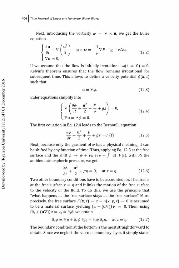
Here, the modulation wavelength K ≈ 0 and the growth ratebecomes algebraic and is not of exponential nature anymore. Thislatter solution is very particular, since it is localized in both spaceand time and it amplifies the amplitude of the carrier theoreticallyby an exact factor of three. A higher-order solution of this kind isreferred to as the Akhmediev–Peregrine solution [29, 34, 35]. Thisdoubly localized solution is characterized by a maximal amplitudeamplification of five (see Fig. 12.2 for an illustration) and is definedby

ψ2 (X , T ) =(

1 + G + i HD

)exp (2 i T ) , (12.52)

Dow

nloa

ded

by [R

yers

on U

nive

rsity

] at 2

1:47

01

Dec

embe

r 201

6



Figure 12.2 (a) First-order doubly localized rational solution (Peregrinebreather), which at X = T = 0 amplifies the amplitude of the carrier by afactor of 3. (b) Second-order doubly localized rational solution (Akhmediev–Peregrine breather), which at X = T = 0 amplifies the amplitude of thecarrier by a factor of 5.

while

G = −(

X 2 + 4T 2 + 34

) (X 2 + 20T 2 + 3

4

)+ 3

4(12.53)

H = 2T(

3X 2 − 4T 2 − 2(

X 2 + 4T 2)2 + 158

)(12.54)

D = 13

(X 2 + 4T 2)3 + 1

4(

X 2 − 12T 2)2

+ 364

(12X 2 + 176T 2 + 1

). (12.55)

All these basic breather solutions, which describe the strongfocusing of a regular background have been only recently observedin Kerr media, water waves and plasma [36–42]. Breathers attractedthe significant scientific interest, since they describe the backbonedynamics of the modulation instability and therefore, of rogue waveas well.

a)

0

3-

.1 -

-5^

X

2

0

-25 T

b)

5

1-5

o'

X

2

0

-25 T

Dow

nloa

ded

by [R

yers

on U

nive

rsity

] at 2

1:47

01

Dec

embe

r 201

6


Experiments of Time Reversal 415

12.2.2.3 Time reversal invariance in the nonlinear regime

The TR invariance of Stokes waves can be discussed withinthe framework of the NLSE. In fact, considering the weaklynonlinear evolution equation (Eq. 12.44), we can notice that thetime-dependent part of the NLSE equation, contains a term ini ∂ E

∂t . Therefore, it is straightforward to see that if E (x , t) is asolution, then its complex conjugate E ∗ (x , −t) is also a solution.Consequently, both surface elevations η (x , t) and η (x , −t) describetwo possible evolutions for the weakly nonlinear water waveproblem. Consequently, a TR mirror can be used to create the time-reversed wave field η (x , −t) in the whole propagating medium. Forthis 1D problem it is sufficient to measure the wave field η (x , t) atone unique point xM and to rebroadcast the time-reversed signalη (xM , −t) from this mirror point in order to observe the solutionη (x , −t) in the whole medium. If this approach is valid for breatherdynamics, it would be a confirmation of the TR invariance of stronglylocalized waves and therefore for nonlinear waves as well.

12.3 Experiments of Time Reversal

In this section we describe recent experiments, confirming the TRinvariance of linear [43] and nonlinear surface gravity waves [44].

12.3.1 Time Reversal of Linear Water WavesIn this section we will start reporting the results of the TR ofwater waves in the linear regime. The experiment is conducted ina water tank cavity to take advantage of multiple reflections onthe boundaries. The influence of the number of channels in the TRmirror is studied and it allows us to show that a small numberof channels is sufficient to obtain the TR refocusing owing to thereverberating effect of the cavity.

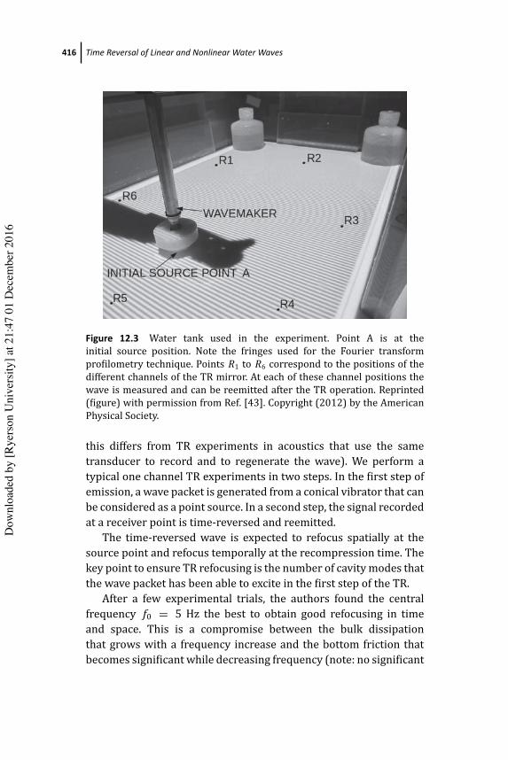
The reverberating tank is filled with water with depth at restH = 10 cm. The dimension of the rectangular tank is 53 × 38 cm2

with obstacles placed in order to break the spatial symmetries(see Fig. 12.3). The waves are generated by using a vertical conicalvibrator and recorded by using an optical method (note that

Dow

nloa

ded

by [R

yers

on U

nive

rsity

] at 2

1:47

01

Dec

embe

r 201

6



Figure 12.3 Water tank used in the experiment. Point A is at theinitial source position. Note the fringes used for the Fourier transformprofilometry technique. Points R1 to R6 correspond to the positions of thedifferent channels of the TR mirror. At each of these channel positions thewave is measured and can be reemitted after the TR operation. Reprinted(figure) with permission from Ref. [43]. Copyright (2012) by the AmericanPhysical Society.

this differs from TR experiments in acoustics that use the sametransducer to record and to regenerate the wave). We perform atypical one channel TR experiments in two steps. In the first step ofemission, a wave packet is generated from a conical vibrator that canbe considered as a point source. In a second step, the signal recordedat a receiver point is time-reversed and reemitted.

The time-reversed wave is expected to refocus spatially at thesource point and refocus temporally at the recompression time. Thekey point to ensure TR refocusing is the number of cavity modes thatthe wave packet has been able to excite in the first step of the TR.

After a few experimental trials, the authors found the centralfrequency f0 = 5 Hz the best to obtain good refocusing in timeand space. This is a compromise between the bulk dissipationthat grows with a frequency increase and the bottom friction thatbecomes significant while decreasing frequency (note: no significant

Rl R2

WAVEMAKERR3

R6

INITIAL SOURCE POINT A

R4.R5

Dow

nloa

ded

by [R

yers

on U

nive

rsity

] at 2

1:47

01

Dec

embe

r 201

6



0 5 10 15 20−10

0

10

t (s)

η (m

m)

a)

0 5 10 150

0.5

1

f (Hz)

η2 (a.

u.)

b)

0 5 10 15 20−10

0

10

t (s)

η (m

m)

c)

0 5 10 150

0.5

1

f (Hz)

η2 (a.

u.)

d)

0 0.2 0.4−10

0

10

t (s)

η (m

m)

0 0.2 0.4−10

0

10

t (s)

η (m

m)

0 5 10 150

0.5

1

f (Hz)

η2 (a.

u.)

0 5 10 150

0.5

1

f (Hz)

η2 (a.

u.)

Figure 12.4 (a) Experimental measurement of the temporal evolutionof the surface elevation, η(r1, t) during the forward propagation afteremission from point A. The inset shows the signal emitted from point A.(b) Corresponding spectrum. The inset shows the spectrum of the signalemitted from point A. (c, d) The same representation from numericalsimulations of the wave equation. Reprinted (figure) with permission fromRef. [43]. Copyright (2012) by the American Physical Society.

peaks in the low-frequency region in Fig. 12.4b). Figure 12.4a showsthe signal recorded at one point (point R1 in Fig. 12.3) when aone-period sinusoidal pulse centered at f0 Hz is generated at theinitial source position. The duration of the signal is typically 20 s,corresponding both to reverberating effects and linear dispersioneffects. This latter is given by the linear dispersion relation for waterwave propagation (taking into account the effects of finite depth Hand surface tension γ ):

ω2 =(

gk + γ

ρk3

)tanh kH , (12.56)

where k denotes the complex wave number, g the gravity accel-eration and ρ the water density. The wavelength at the central

Dow

nloa

ded

by [R

yers

on U

nive

rsity

] at 2

1:47

01

Dec

embe

r 201

6



frequency f0 is λ = 6 cm. The magnitude of nonlinearity ofthe waves based on the maximum measured gradient of surfaceelevation was found to be ϵ = 0.13. The attenuation is such thatthe wave can propagate over roughly 100 wavelengths, that is, about10 to 20 times the length scale of the cavity. This is consistent withthe 20 s duration of the time signal recorded at one point inthe cavity (Fig. 12.4a) since the phase velocity at the centralfrequency is 0.33 m/s corresponding to 12–17 reflections from theboundaries. The spectrum of the signal recorded during the directpropagation is shown in Fig. 12.4b. It presents several peaks (onecan count roughly 20 peaks) corresponding to the eigenmodes ofthe cavity that have been excited. Although the initial pulse covers abroadband frequency range [0 15] Hz, the signal recorded is limitedto frequencies smaller than about 10 Hz. We have checked that this isan effect of the attenuation: direct numerical simulations of the 2Dwave equation in the same geometry but omitting the attenuationgive a spectrum with around 100 cavity modes excited in the wholerange 0 15 Hz (Fig 12.4c,d).

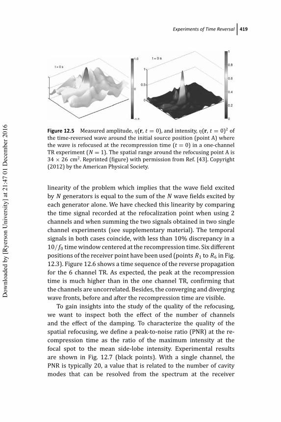
We now investigate the refocusing. The perturbation of thesurface elevation η(r, t) is measured in time and in space duringthe wave propagation using an optical method (FTP for Fouriertransform profilometry) that has been adapted recently to waterwave measurements [45–48]. FTP is used to measure the wholepattern of surface elevation η(r, t) at each time of the reversepropagation. This has been done in one-channel experiments (N =1). Although the spatial refocusing and temporal recompression arevisible (Fig. 12.5), it is not possible to distinguish the convergingwave fronts before the recompression and the diverging wave frontsafter recompression in this one channel experiments (for a movie,see the supplementary material).

To improve the refocusing, it is possible to increase the numberof channels. In a TR experiments with multiple channels, the signalemitted from the source point is recorded at N receiver points. TheTR signal are then reemitted simultaneously from the N receiverpoints. If the N receiver points are uncorrelated, it is meant toimprove the refocusing since the wave experiences many differenttrajectories in the cavity. In our experiment, rather than using Nwave generators to reemit the signal, the N channel TR have beendone with just one wave generator. This is possible by exploiting the

Dow

nloa

ded

by [R

yers

on U

nive

rsity

] at 2

1:47

01

Dec

embe

r 201

6



Figure 12.5 Measured amplitude, η(r, t = 0), and intensity, η(r, t = 0)2 ofthe time-reversed wave around the initial source position (point A) wherethe wave is refocused at the recompression time (t = 0) in a one-channelTR experiment (N = 1). The spatial range around the refocusing point A is34 × 26 cm2. Reprinted (figure) with permission from Ref. [43]. Copyright(2012) by the American Physical Society.

linearity of the problem which implies that the wave field excitedby N generators is equal to the sum of the N wave fields excited byeach generator alone. We have checked this linearity by comparingthe time signal recorded at the refocalization point when using 2channels and when summing the two signals obtained in two singlechannel experiments (see supplementary material). The temporalsignals in both cases coincide, with less than 10% discrepancy in a10/ f0 time window centered at the recompression time. Six differentpositions of the receiver point have been used (points R1 to R6 in Fig.12.3). Figure 12.6 shows a time sequence of the reverse propagationfor the 6 channel TR. As expected, the peak at the recompressiontime is much higher than in the one channel TR, confirming thatthe channels are uncorrelated. Besides, the converging and divergingwave fronts, before and after the recompression time are visible.

To gain insights into the study of the quality of the refocusing,we want to inspect both the effect of the number of channelsand the effect of the damping. To characterize the quality of thespatial refocusing, we define a peak-to-noise ratio (PNR) at the re-compression time as the ratio of the maximum intensity at thefocal spot to the mean side-lobe intensity. Experimental resultsare shown in Fig. 12.7 (black points). With a single channel, thePNR is typically 20, a value that is related to the number of cavitymodes that can be resolved from the spectrum at the receiver

lo.s

0.5

3.4

r'o

T = D SL o

0.5*

oJ

0

„

1 - 0 - z

Dow

nloa

ded

by [R

yers

on U

nive

rsity

] at 2

1:47

01

Dec

embe

r 201

6



Figure 12.6 Space–time-resolved experimental measurements of the sur-face elevation η(r, t) during the refocusing of the time-reversed wave. Inthis case, N = 6 channels (points R1 to R6) reemit the time-reversedsignals. The recompression time is at t = 0 s. Converging and divergingwave fronts appear respectively for negative and positive times. The spatialrange around the refocusing point A is 34 × 26 cm2. Reprinted (figure)with permission from Ref. [43]. Copyright (2012) by the American PhysicalSociety.

point in Fig. 12.4. With several channels, the PNR increases linearlywith the number N of channels [49]. Although this behavior isexpected without damping, it was not obvious to be verified with thetypical range of damping of our experiment. The insets of Fig. 12.7

ro

'-0.3

ro

i.,iO,3

0

'-0.3

t = 0.56 s

t =-0.56st = -1,12sU3

0

0.3

t = -0,4 S t = 0s

"Io-

Jt = 0 ,4s

0 3

0

-0.3

Dow

nloa

ded

by [R

yers

on U

nive

rsity

] at 2

1:47

01

Dec

embe

r 201

6



1 2 3 4 5 6 70

100

200

300

400

500

600

700

Number of reemiters

peak

inte

nsity

/ no

ise

inte

nsity

−2 0 2−10

0

10

t (s)

η (m

m)−2 0 2

−2

0

2

t (s)

η (m

m)

Figure 12.7 Experimentally measured peak-to-noise ratio as a functionof the number N of channels (black points). For comparison, the bluesquares show numerical results with negligible damping. Note the standarddeviation accounting for the sensitivity of the refocusing to the positionof the reemission point. The insets present the experimental temporalrefocalization while using one and six channels. Reprinted (figure) withpermission from Ref. [43]. Copyright (2012) by the American PhysicalSociety.

show the temporal recompression for N = 1 and N = 6 at therefocusing point A. The refocusing is clearly visible in the one-channel TR experiment but with higher temporal side lobes thanwith 6 channels. Note that these temporal signals allow also todefine a PNR and we observed that PNR either defined in spaceor in time have roughly the same values. Varying the damping ismore difficult. To perform experiments where the damping effect isnegligible would necessitate much larger size of the cavity (e.g., thesize of a swimming pool) because the attenuation per wavelengthdecreases with the frequency [9]. Therefore, numerical simulationshave been used to model the case with negligible damping. Theresults are shown in Fig. 12.7 (blue square) where computationshave been done by taking the same protocol as in the experiment.The same trends as in the experiment are observed: i) for N = 1,

Dow

nloa

ded

by [R

yers

on U

nive

rsity

] at 2

1:47

01

Dec

embe

r 201

6



the PNR is equal to 100 and is given by the number of excitedcavity modes that can be resolved in the spectrum in Fig. 12.4, ii)the PNR increases linearly with N . With about 20 excited modes inour laboratory experiments, versus the 100 modes obtained in thenumerics, it appears that the refocusing can be significantly reducedbecause of the attenuation occurring at that laboratory scale.

Our experiments illustrate the feasibility of a few channel TRrefocusing for gravity capillary waves. This has been performedin a well-controlled laboratory context that allows quantitativemeasurements simultaneously in time and space. At this laboratoryscale, with centimetric wavelengths, the quality of the refocusingis limited by the damping due to viscous effects but it is notsuppressed. At larger scales, viscous damping highly decreases andnumerical simulations show that the refocusing is greatly improved.Thus, this paves the way to applications in the context of waterwaves in the sea, with very small damping, where very high qualityof refocusing is expected.

12.3.2 Time Reversal of Nonlinear Water WavesNext, an experimental demonstration of TR of nonlinear waves ispresented. Due to the strong nonlinear focusing of NLSE breathers,the doubly localized Peregrine and the higher-order Akhmediev–Peregrine breathers solutions will be used for the demonstration inone spatial direction of wave propagation. Following the 1D NLSE(Eq. 12.44), the experiments, performed in a unidirectional wavebasin, are first started by generating the maximal amplitude ofhydrodynamic and doubly localized breather by the wave maker,which is considered to be the source of the propagation. Its positionis labeled by xS . The attenuated breather-type wave field is thenmeasured at the mirror position, labeled by xM , after a specificpropagation distance. The collected signal is then reversed in time,providing new initial conditions to a wave generator. As for thelinear experiment, if the TR symmetry is valid, one should expectthe refocusing and the perfect reconstruction of the initial maximalbreather compression, after reemitting the time-reversed signal.Due to the experimental limitations with respect to the generationof the time-reversed signal at the mirror position, we will use

Dow

nloa

ded

by [R

yers

on U

nive

rsity

] at 2

1:47

01

Dec

embe

r 201

6



the spatial reciprocity of the NLSE in order to reemit the time-reversed surface elevation signal of the attenuated breather from thesource and observe the refocusing at the mirror position xM , insteadof rebroadcasting the reversed wave field from xM and expectingrefocusing at the source position xS .

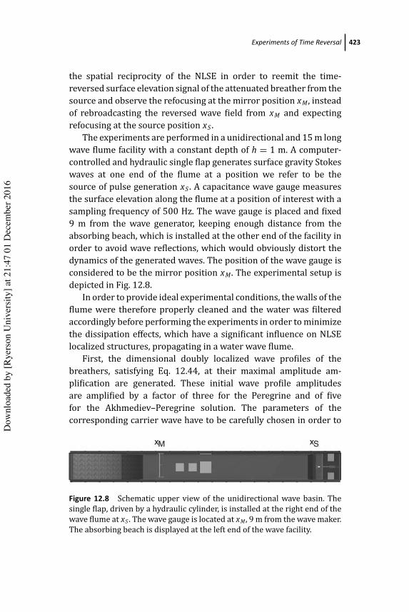
The experiments are performed in a unidirectional and 15 m longwave flume facility with a constant depth of h = 1 m. A computer-controlled and hydraulic single flap generates surface gravity Stokeswaves at one end of the flume at a position we refer to be thesource of pulse generation xS . A capacitance wave gauge measuresthe surface elevation along the flume at a position of interest with asampling frequency of 500 Hz. The wave gauge is placed and fixed9 m from the wave generator, keeping enough distance from theabsorbing beach, which is installed at the other end of the facility inorder to avoid wave reflections, which would obviously distort thedynamics of the generated waves. The position of the wave gauge isconsidered to be the mirror position xM . The experimental setup isdepicted in Fig. 12.8.

In order to provide ideal experimental conditions, the walls of theflume were therefore properly cleaned and the water was filteredaccordingly before performing the experiments in order to minimizethe dissipation effects, which have a significant influence on NLSElocalized structures, propagating in a water wave flume.

First, the dimensional doubly localized wave profiles of thebreathers, satisfying Eq. 12.44, at their maximal amplitude am-plification are generated. These initial wave profile amplitudesare amplified by a factor of three for the Peregrine and of fivefor the Akhmediev–Peregrine solution. The parameters of thecorresponding carrier wave have to be carefully chosen in order to

Figure 12.8 Schematic upper view of the unidirectional wave basin. Thesingle flap, driven by a hydraulic cylinder, is installed at the right end of thewave flume at xS . The wave gauge is located at xM , 9 m from the wave maker.The absorbing beach is displayed at the left end of the wave facility.

xm Xs

Dow

nloa

ded

by [R

yers

on U

nive

rsity

] at 2

1:47

01

Dec

embe

r 201

6



avoid initial wave breaking of obviously strongly nonlinear focusedwaves at xS and in order to reach satisfactory attenuation after9 m of propagation. Consequently, the carrier wave parameters,determined by the steepness ε and the amplitude a, have to bechosen accordingly. Both parameters are set to be ε = 0.09 anda = 3 mm for the Peregrine as well as ε = 0.03 and a = 1 mm for theAkhmediev–Peregrine solution. These chosen steepness values arefar from the experimentally determined wave breaking thresholds[50]. The steepness ε and the amplitude a of the Stokes backgroundare sufficient to determine the carrier parameters. Trivially, thewave number is k = ε

a . The linear dispersion relation of deepwater determine the wave frequency to be ω =

√gk, while denotes

the gravitational acceleration and is g = 9.81 m · s−2. The initialconditions are then trivially determined by

η(x∗, t) = Re (E (x∗, t) · exp [i (kx∗ − ωt)]) , (12.57)

evaluated at x∗ = 0, in order to satisfy the maximal breathercompression. Figure 12.9 shows the initial conditions applied to theflap at the Position xS .

After generating the Peregrine and the Akhmediev–Peregrinebreather at their maximal wave amplitude of 0.9 cm and 0.5 cm,respectively, we collect the wave profiles after having being declinedin amplitude, as expected and predicted by theory, by use of the wavegauge at xM , that is, 9 m from the flap Position xS . Here, we noticealready a deviation from theoretical weakly nonlinear wave profiles,due to the strongly nonlinear nature of the initially generated waveforms. These discrepancies can be explained by higher-order NLSE,known as the modified NLSE [20]. The corresponding data areshown in Fig. 12.10a,b.

In the third step these recorded breather signals are revisedin time. These time-reversed signals provide now new initialconditions to the flap in order to initiate the fourth and penultimatestage of the TR experiment. The latter are depicted in Fig.12.10c,d. If the considered breather dynamics is indeed TR invariant,it is expected to observe the refocusing of the maximal wavecompressions after reemitting the latter time-reversed and slightlymodulated signals to the wave maker. Here, we take advantage ofthe spatial reciprocity of the NLSE equation, thus, we can reemit the

Dow

nloa

ded

by [R

yers

on U

nive

rsity

] at 2

1:47

01

Dec

embe

r 201

6



0 10 20 30 40−9

−3

3

9

t (s)

0 10 20 30 40

−5

−1

1

5

t (s)

η (m

m)

a)

b)

Figure 12.9 Initial conditions provided by theory (Eq. 12.45) at the positionof maximal amplification, that is, at X = 0, applied to the wave flap atPosition xS . (a) The carrier parameters for the Peregrine breather-typewater wave profile are a0 = 0.3 cm and ε = 0.09. (b) The carrier parametersfor the Akhmediev–Peregrine breather-type water wave profile are a0 =0.1 cm and ε = 0.03.

time-reversed signal from the point xS and observe the refocusing atpoint xM , rather than rebroadcasting the reversed wave field from xM

and expecting refocusing at the position xS . At the fifth and last stepof the experiments, we measure the surface elevations related to thetime-reversed initial conditions, again 9 m from the flap at positionxM , that is, keeping the wave gauge at the same position. Theserefocused measurements are compared to the theoretical surfaceelevations. The corresponding wave profiles are shown in Fig. 12.11.

These results are a clear demonstration of the TR invariance ofthe hydrodynamic breathers. Clearly, Fig. 12.11 provides an accuraterefocusing and reconstruction of the breather surface elevationof the corresponding NLSE solution at its maximal compression,as already presented in Fig. 12.9. The results are in a very good

Dow

nloa

ded

by [R

yers

on U

nive

rsity

] at 2

1:47

01

Dec

embe

r 201

6



0 10 20 30 40

−3

3

9

t (s)

0 10 20 30 40

−3

3

9

t (s)

η (m

m) 0 10 20 30 40

−1

1

5

t (s)

0 10 20 30 40

−1

1

5

t (s)

η (m

m)

a) b)

c) d)

Figure 12.10 (a) Surface elevation of water wave profile of the attenuatedPeregrine breather, recorded at xM , located 9 m form the flap. (b) Surfaceelevation of water wave profile of the attenuated Akhmediev–Peregrinebreather, recorded at xM , located 9 m form the flap. (c) Time-reversed signalof the measurements shown in (a), providing new initial conditions to theflap and reemitted at xS . (d) Time-reversed signal of the measurementsshown in (b), providing new initial conditions to the flap and reemitted atxS .

agreement with the theoretical predictions, expected at this positionwithin the framework of NLSE. In fact, the maximal water surfaceamplitude is of 9 mm and of 5 mm for the Peregrine breather andthe Akhmediev–Peregrine breather, respectively, which correspondto theoretical values of amplitude amplifications, related to theseNLSE solutions at the maximal stage of breather compression andas generated in the first step of the experiment. These observationsprove the TR invariance of strongly nonlinear water waves. In ad-dition, these experimental results confirm the accuracy of the NLSEin describing the unidirectional and complex evolution dynamics ofrogue waves, taking into account the complex phase-shift dynamics,

Dow

nloa

ded

by [R

yers

on U

nive

rsity

] at 2

1:47

01

Dec

embe

r 201

6



0 5 10 15 20

39

39

t (s)

0 5 10 15 20 25 30

1

5

1

5

t (s)

η (m

m)

a)

b)

Figure 12.11 (a) Comparison of the Peregrine surface profile measured9 m from the paddle at xM , while starting its propagation from time-reversed initial conditions (blue upper line) with the expected theoreticalNLSE prediction at the same position (red bottom line). (b) Comparison ofthe Akhmediev–Peregrine surface profile measured 9 m from the paddleat Position xM , while starting its propagation from time-reversed initialconditions (blue upper line) with the expected theoretical NLSE predictionat the same position (red bottom line).

related to the modulation instability process. Nevertheless, somediscrepancies between theory and experiment can be also notedin terms of asymmetric wave profile shape of the experimentalobservations, as can be noticed in Fig. 12.11. The latter are dueto higher-order nonlinearities (Stokes drift) and to higher-orderdispersion effects, not taken into account in the NLSE approach,as well as to occurring experimental imperfections, including dis-sipation and wave reflection and most importantly noise, naturallyand always existing while performing experiments in wave basins.Nevertheless, the experimental observations confirm the possibilityto reconstruct strongly localized, thus, strongly nonlinear waves

Dow

nloa

ded

by [R

yers

on U

nive

rsity

] at 2

1:47

01

Dec

embe

r 201

6



through TR. Therefore, we emphasize that this technique may beused in order to construct new TR invariant localized structures,described by nonlinear evolution equations, which considerablyamplify the amplitude of a wave field, thus, again also in the caseof strong nonlinearity.

12.4 Discussion and Outlook

Experiments on water wave pulse field reconstruction in the linearand nonlinear regime using TR, provide not only a confirmationof the TR invariance of the hydrodynamic wave motion, but alsoopen new field of possible applications in several dispersive media.This includes, for example, superfluidity [51, 52] and optical fibers[15, 53]. The experiments, involving the doubly localized breathersolutions of the NLSE show also limitations, which should beaddressed. First, discrepancies with respect to the theoreticalNLSE predictions can be noticed. These can be easily explained inview of the natural limitation of the NLSE. A successive analysiscould be performed in order to verify the TR invariance, alsofor higher-order NLSE-type evolution equation [20, 56] as well aswithin the framework of fully nonlinear equations [55]. This isto accurately characterize possible applications and limitations ofthe TR method for nonlinear, very steep, and nonbreaking waterwaves. Another interesting point, which should be addressed froma chaotic dynamics point view is the influence of random noiseon the TR reconstruction of NLSE breathers. Next, we inspect thenumerical instability of the TR scheme, by perturbing the initialconditions of the same nonlinear experiments within the frameworkof the NLSE. We used the split-step Fourier method [57, 58] toillustrate the influence of the random noise on the decaying andTR reconstruction dynamics of both, Peregrine and Akhmediev–Peregrine dynamics for the same wave parameters as used in thelaboratory experiments. The initial conditions have been multipliedby [1 + N2(t)] [59]. Here, 2 is a normally distributed randomfunction, whereas N denotes the noise level, which is chosen tobe 10−1 and 10−2, respectively. The numerical results involvingthe Peregrine breather for the same laboratory parameters over a

Dow

nloa

ded

by [R

yers

on U

nive

rsity

] at 2

1:47

01

Dec

embe

r 201

6


Discussion and Outlook 429

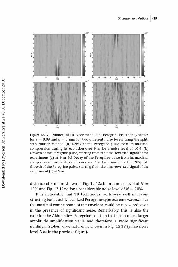
Figure 12.12 Numerical TR experiment of the Peregrine breather dynamicsfor ε = 0.09 and a = 3 mm for two different noise levels using the split-step Fourier method. (a) Decay of the Peregrine pulse from its maximalcompression during its evolution over 9 m for a noise level of 10%. (b)Growth of the Peregrine pulse, starting from the time-reversed signal of theexperiment (a) at 9 m. (c) Decay of the Peregrine pulse from its maximalcompression during its evolution over 9 m for a noise level of 20%. (d)Growth of the Peregrine pulse, starting from the time-reversed signal of theexperiment (c) at 9 m.

distance of 9 m are shown in Fig. 12.12a,b for a noise level of N =10% and Fig. 12.12c,d for a considerable noise level of N = 20%.

It is noticeable that TR techniques work very well in recon-structing both doubly localized Peregrine-type extreme waves, sincethe maximal compression of the envelope could be recovered, evenin the presence of significant noise. Remarkably, this is also thecase for the Akhmediev–Peregrine solution that has a much largeramplitude amplification value and therefore, a more significantnonlinear Stokes wave nature, as shown in Fig. 12.13 (same noiselevel N as in the previous figure).

Dow

nloa

ded

by [R

yers

on U

nive

rsity

] at 2

1:47

01

Dec

embe

r 201

6



Figure 12.13 Numerical TR experiment of the Akhmediev–Peregrinebreather dynamics for ε = 0.03 and a = 1 mm for two different noise levelsusing the split-step Fourier method. (a) Decay of the Akhmediev–Peregrinepulse from its maximal compression during its evolution over 9 m for anoise level of 10%. (b) Growth of the Peregrine pulse, starting from the time-reversed signal of the experiment (a) at 9 m. (c) Decay of the Akhmediev–Peregrine pulse from its maximal compression during its evolution over9 m for a noise level of 20%. (d) Growth of the Akhmediev–Peregrine pulse,starting from the time-reversed signal of the experiment (c) at 9 m.

Another possible application is the validation of TR recon-struction of nonlinear waves, propagating in two spatial directions[60, 61]. Deep-water evolutions equations, such as the Davey–Stewartson equation [62] or the shallow water KP-I [63] could beused for this investigation. Obviously, experiments for such type ofequations are much more difficult to perform. Furthermore, newpossible solutions may be derived numerically in the limit of TRconvergence.

Dow

nloa

ded

by [R

yers

on U

nive

rsity

] at 2

1:47

01

Dec

embe

r 201

6


References 431

12.5 Conclusion

To summarize, we have discussed the TR invariance of surfacegravity water waves in the linear and nonlinear regime. Afterintroducing the governing equations of an ideal fluid and empha-sizing the conditions for the TR invariance, we have presentedrecent experiments, validating the TR approach in reconstructinglinear and 2D water pulses, whereas two examples of nonlinearbreather-type pulses have been refocused in a 1D water wave flume.The experimental results provide a clear confirmation of the TRinvariance of water waves and emphasize novel applications inother dispersive media, such as fiber optics, plasma and Bose–Einstein condensates as well as in remote sensing to name onlyfew. The effect of dynamical noise on the nonlinear breather wavepropagation has been discussed numerically as well. The reportedsimulations, based on the split-step Fourier method are promisingand motivate further analytical, numerical and experimental work inanalyzing the hydrodynamics and complex propagation propertiesof linear and nonlinear waves, using the TR technique.

References

1. Fink, M. (1997). Phys. Today, 3, 34.

2. Lerosey, G., de Rosny, J., Tourin, A., Derode, A., Montaldo, G., and Fink, M.(2004). Phys. Rev. Lett., 92, 193904.

3. Fink, M., Cassereau, D., Derode, A., Prada, C., Roux, P., Tanter, M., Thomas,J.-L., and Wu, F. (2000). Rep. Prog. Phys., 63, 1933.

4. Draeger, C., and Fink, M. (1997). Phys. Rev. Lett., 79, 407.

5. Feynman, R.P., Leighton, R.B., and Sands, M. (1963). The FeynmanLectures on Physics, Vol. I, Chaps. 51–54 (Addison-Wesley, Reading, MA).

6. Roux, P. and Fink, M. (2000). J. Acoust. Soc. Am., 107, 2418–2429.

7. Ing, R.K. and Fink, M. (1998). IEEE Trans. Ultrason. Ferroelectr. Freq.Control, 45, 1032.

8. Tanter, M., Thomas, J.-L., Coulouvrat, F., and Fink, M. (2001). Phys. Rev. E,64, 016602.

9. Lighthill, J. (2001). Waves in Fluids (Cambridge University Press).

Dow

nloa

ded

by [R

yers

on U

nive

rsity

] at 2

1:47

01

Dec

embe

r 201

6



10. Mei, C.C., Stiassnie, M.M., and Yue, D.K.P. (2005). Theory and Applicationsof Ocean Surface Waves, Advanced Series on Ocean Engineering, Vol. 23.

11. Osborne, A. (2010). Nonlinear Ocean Waves & the Inverse ScatteringTransform, Vol. 97 (Academic Press).

12. Kharif, C., Pelinovsky, E., and Slunyaev, A. (2009). Rogue Waves in theOcean (Springer).

13. Dalrymple, R.A., and Dean, R.G. (1991). Water Wave Mechanics forEngineers and Scientists (Prentice Hall).

14. Linton, C.M., and McIver, P. (2001). Handbook of Mathematical Tech-niques for Wave/Structure Interactions (CRC Press).

15. Remoissenet, M. (1999). Waves Called Solitons (Springer).

16. Debnath, L. (1994). Nonlinear Water Waves (Academic Press).

17. Stokes, G.G. (1847). On the theory of oscillatory waves, Trans. Camb.Philos. Soc., 8, 441–455.

18. Benjamin, T.B. and Feir, J.E. (1967)The disintegration of wave trains ondeep water. Part 1. Theory, J. Fluid Mech., 27, 417–430.

19. Zakharov, V.E. (1968). Stability of periodic waves of finite amplitude ona surface of deep fluid, J. Appl. Mech. Tech. Phys., 9, 190–194.

20. Dysthe, K.B. (1979). Note on the modification of the nonlinearSchrodinger equation for application to deep water waves, Proc. R. Soc.A, 369, 105–114.

21. Zakharov, V.E. and Shabat, A.B. (1972). Exact theory of two-dimensionalself-focusing and one-dimensional self-modulation of waves in nonlin-ear media, J. Exp. Theor. Phys., 34, 62–69.

22. Bespalov, V.I., and Talanov, V.I. (1966). Filamentary structure of lightbeams in nonlinear liquids, JETP Lett., 3, 307–310.

23. Lake, B.M., and Yuen, H.C. (1977). Note on some nonlinear water-waveexperiments and the comparison of data with theory, J. Fluid Mech., 83,75–81.

24. Benjamin, T.B. (1967). Instability of periodic wavetrains in nonlineardispersive systems, Proc. R. Soc. A., 299, 59–75.

25. Zakharov, V.E. and Ostrovsky, L.A. (2009). Modulation instability: thebeginning, Physica D, 238, 540–548.

26. Hasimoto, H., and Ono, H. (1972). Nonlinear modulation of gravitywaves, J. Phys. Soc. Jpn., 33, 805–811.

27. Yuen, H.C., and Lake, B.M. (1982). Nonlinear dynamics of deep-watergravity waves, Adv. Appl. Mech., 22, 67–229.

Dow

nloa

ded

by [R

yers

on U

nive

rsity

] at 2

1:47

01

Dec

embe

r 201

6


References 433

28. Tulin, M.P., and Waseda, T. (1999). Laboratory observations of wavegroup evolution, including breaking effects, J. Fluid Mech., 378, 197–232.

29. Akhmediev, N., Eleonskii, V.M., and Kulagin, N. (1985). Generationof periodic sequence of picosecond pulses in an optical fibre: exactsolutions, J. Exp. Theor. Phys., 61, 894–899.

30. Akhmediev, N., and Korneev, V.I. (1986). Modulation instability andperiodic solutions of the nonlinear Schrodinger equation, Theor. Math.Phys., 69, 1089–1093.

31. Kuznetsov, E.A. (1977). Solitons in a parametrically unstable plasma,Sov. Phys. Dokl., 22, 507–508.

32. Ma, Y.C. (1979). The perturbed plane wave solutions of the cubicnonlinear Schrodinger equation, Stud. Appl. Math., 60, 43–58.

33. Peregrine, D.H. (1983). Water waves, nonlinear Schrodinger equationsand their solutions, J. Aust. Math. Soc. Ser. B, 25, 16–43.

34. Akhmediev, N., Ankiewicz, A., and Soto-Crespo, J.M. (2009). Rogue wavesand rational solutions of the nonlinear Schrodinger equation, Phys. Rev.E, 80, 026601.

35. Akhmediev, N., Ankiewicz, A., and Taki, M. (2009). Waves that appearfrom nowhere and disappear without a trace, Phys. Lett. A, 373, 675–678.

36. Dudley, J.M., Genty, G., Dias, F., Kibler, B., and Akhmediev, N. (2009).Modulation instability, Akhmediev breathers and continuous wavesupercontinuum generation, Opt. Express, 17, 21497.

37. Kibler, B., Fatome, J., Finot, C., Millot, G., Dias, F., Genty, G., Akhmediev, N.,and Dudley, J.M. (2010). The Peregrine soliton in nonlinear fibre optics,Nat. Phys., 6, 790–795.

38. Chabchoub, A., Hoffmann, N.P., and Akhmediev, N. (2011). Rogue waveobservation in a water wave tank, Phys. Rev. Lett., 106, 204502.

39. Chabchoub, A., Hoffmann, N., Onorato, M., and Akhmediev, N. (2012).Super rogue waves: observation of a higher-order breather in waterwaves, Phys. Rev. X, 2, 011015.

40. Bailung, H., Sharma, S.K., and Nakamura, Y. (2011). Observation ofPeregrine solitons in a multicomponent plasma with negative ions, Phys.Rev. Lett., 107, 255005.

41. Onorato, M., Proment, D., Clauss, G., and Klein, M. (2013). Rogue waves:from nonlinear Schrodinger breather solutions to sea-keeping test,PLOS ONE, 8, e54629.

Dow

nloa

ded

by [R

yers

on U

nive

rsity

] at 2

1:47

01

Dec

embe

r 201

6



42. Chabchoub, A., Kibler, B., Dudley, J.M., and Akhmediev, N. (2014).Hydrodynamics of periodic breathers, Phil. Trans. R. Soc. A, 372,20140005.

43. Przadka, A., Feat, S., Petitjeans, P., Pagneux, V., Maurel, A., and Fink, M.(2012). TR of water waves, Phys. Rev. Lett., 109, 064501.

44. Chabchoub, A., and Fink, M. (2014). Time-reversal generation of roguewaves, Phys. Rev. Lett., 112, 124101.

45. Maurel, A., Cobelli, P., Pagneux, V., and Petitjeans, P. (2009). J. Appl. Opt.,48, 380; Cobelli, P., Maurel, A., Pagneux, V., and Petitjeans, P. (2009). Exp.Fluids, 46, 1037.

46. Recent improvements of the technique for signal processing and thechoice of painting particles can be found, respectively, in G. Lagubeauet al., in preparation; Przadka, A., Cabane, B., Pagneux, V., Maurel, A., andPetitjeans, P. (2012). Exp. Fluids, 52, 519.

47. Cobelli, P., Petitjeans, P., Maurel, A., Pagneux, V., and Mordant, N. (2009).Phys. Rev. Lett., 103, 204301.

48. Cobelli, P., Pagneux, V., Maurel, A., and Petitjeans, P. (2009). Europhys.Lett., 88, 20006; (2011). J. Fluid Mech., 666, 445–476.

49. Draeger, C., and Fink, M. (1999). J. Acoust. Soc. Am., 105, 611.

50. Chabchoub, A., Hoffmann, N., Onorato, M., Slunyaev, A., Sergeeva, A.,Pelinovsky, E., and Akhmediev, N. (2012). Observation of a hierarchy ofup to fifth-order rogue waves in a water tank, Phys. Rev. E, 86, 056601.

51. Gross, E.P. (1961). Structure of a quantized vortex in boson systems, IlNuovo Cimento, 20, 454–457.

52. Pitaevskii, L.P. (1961). Vortex lines in an imperfect Bose gas, Sov. Phys.JETP, 13, 451–454.

53. Dudley, J.M., Dias, F., Erkintalo, M., and Genty, G. (2014). Instabilities,breathers and rogue waves in optics, Nat. Photon., 8, 755–764.

54. Craig, W., Guyenne, P., and Sulem, C. (2010). Hamiltonian approach tononlinear modulation of surface water waves, Wave Motion, 47, 552–563.

55. (2013). On the highest non-breaking wave in a group: fully nonlinearwater wave breathers versus weakly nonlinear theory, J. Fluid Mech.,735, 203–248.

56. Craig, W., Guyenne, P., and Sulem, C. (2010). Hamiltonian approach tononlinear modulation of surface water waves, Wave Motion, 47, 552–563.

57. Hardin, R.H., and Tappert, F.D. (1973). SIAM Rev. Chronicle, 15, 423.

Dow

nloa

ded

by [R

yers

on U

nive

rsity

] at 2

1:47

01

Dec

embe

r 201

6


References 435

58. Fisher, R.A., and Bischel, W.K. (1975). Appl. Phys. Lett., 23, 661 (1973); J.Appl. Phys., 46, 4921.

59. Chen, S., Soto-Crespo, J.M., and Grelu, P. (2014). Dark three-sister roguewaves in normally dispersive optical fibers with random birefringence,Opt. Express, 22, 27632–27642.

60. Waseda, T., Kinoshita, T., and Tamura, H. (2009). Evolution of a randomdirectional wave and freak wave occurrence, J. Phys. Oceanogr., 38, 621–639.

61. Toffoli, A., Gramstad, O., Trulsen, K., Monbaliu, J., Bitner-Gregersen,E., and Onorato, M. (2010). Evolution of weakly nonlinear randomdirectional waves: laboratory experiments and numerical simulations,J. Fluid. Mech., 313–336.

62. Davey, A., and Stewartson, K. (1974). On three dimensional packets ofsurface waves, Proc. R. Soc. A, 338, 101–110.

63. Kadomtsev, B.B., and Petviashvili, V.I. (1970). On the stability of solitarywaves in weakly dispersive media, Sov. Phys. Dokl., 15, 539–541.

Dow

nloa

ded

by [R

yers

on U

nive

rsity

] at 2

1:47

01

Dec

embe

r 201

6

Dow

nloa

ded

by [R

yers

on U

nive

rsity

] at 2

1:47

01

Dec

embe

r 201

6

http://www.taylorandfrancis.com

Chapter 12 Time Reversal of Linear and Nonlinear Water Waves · August 1, 2016 15:7 PSP Book - 9in...

Documents

Transcript of Chapter 12 Time Reversal of Linear and Nonlinear Water Waves · August 1, 2016 15:7 PSP Book - 9in...