Chapter 10 Estimating the Binomial Tree. Before we describe the models for estimating binomial...
104
Chapter 10 Estimating the Binomial Tree
-
Upload
valentine-carson -
Category
Documents
-
view
223 -
download
6
Transcript of Chapter 10 Estimating the Binomial Tree. Before we describe the models for estimating binomial...

Chapter 10Chapter 10
Estimating the Binomial TreeEstimating the Binomial Tree

Estimating the Binomial TreeEstimating the Binomial Tree
• Before we describe the models for estimating binomial interest rate trees, we first need to look at how we can subdivide the tree so that the assumed binomial process is defined in terms of a realistic length of time, with a sufficient number of possible rates at maturity.
• Before we describe the models for estimating binomial interest rate trees, we first need to look at how we can subdivide the tree so that the assumed binomial process is defined in terms of a realistic length of time, with a sufficient number of possible rates at maturity.

Subdividing the Binomial TreeSubdividing the Binomial Tree
• The binomial model is more realistic when we subdivide the periods to maturity into a number of subperiods.
• As the number of subperiods increases:– The length of each period becomes smaller, making the
assumption that the spot rate will either increase or decrease more plausible.
– The number of possible rates at maturity increases, which again adds realism to the model.

Subdividing the Binomial TreeSubdividing the Binomial Tree
• Suppose the three-period bond in our illustrative example were a three-year bond.
• Instead of using a three-period binomial tree, where the length of each period is a year, suppose we evaluate the bond using a six-period tree with the length of each period being six months.
• If we do this, we need to:
– Divide the one-year spot rates and the annual coupon by two.
– Adjust the u and d parameters to reflect changes over a six-month period instead of one year.
– Define the binomial tree of spot rates for five periods, each with a length of six months.

Subdividing the Binomial TreeSubdividing the Binomial Tree
• In general, let: – h = length of the period in years– n = number of periods of length h defining
the maturity of the bond• where n = (maturity in years)/h
• In general, let: – h = length of the period in years– n = number of periods of length h defining
the maturity of the bond• where n = (maturity in years)/h
Subdividing the Binomial TreeSubdividing the Binomial Tree
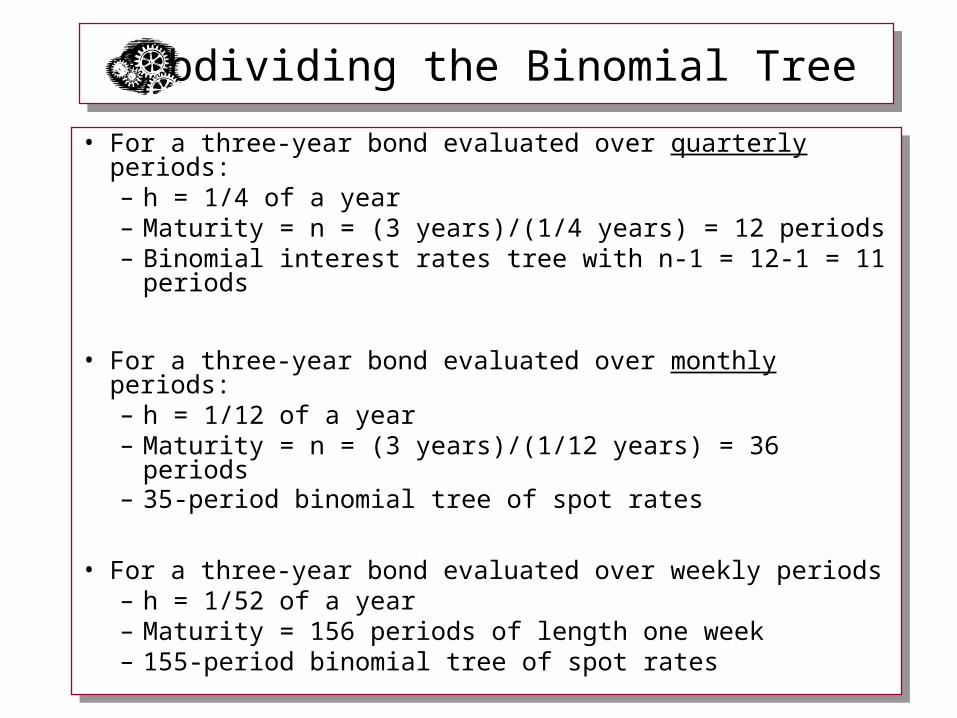
• For a three-year bond evaluated over quarterly periods:– h = 1/4 of a year – Maturity = n = (3 years)/(1/4 years) = 12 periods – Binomial interest rates tree with n-1 = 12-1 = 11 periods
• For a three-year bond evaluated over monthly periods:– h = 1/12 of a year– Maturity = n = (3 years)/(1/12 years) = 36 periods – 35-period binomial tree of spot rates
• For a three-year bond evaluated over weekly periods – h = 1/52 of a year– Maturity = 156 periods of length one week– 155-period binomial tree of spot rates

Subdividing the Binomial TreeSubdividing the Binomial Tree
• Thus, by subdividing we make the length of each period smaller, which makes the assumption of only two possible rates at the end of one period more plausible, and we increase the number of possible rates at maturity.
• Thus, by subdividing we make the length of each period smaller, which makes the assumption of only two possible rates at the end of one period more plausible, and we increase the number of possible rates at maturity.

Estimating the Binomial TreeEstimating the Binomial Tree
• There are two general approaches to estimating binomial interest rate movements. 1. Estimating the u and d Parameters –
Equilibrium Model
2. Calibration Model – Arbitrage-Free Model
• There are two general approaches to estimating binomial interest rate movements. 1. Estimating the u and d Parameters –
Equilibrium Model
2. Calibration Model – Arbitrage-Free Model

Binomial Interest Rate Models
u and d Estimation Approach - Equilibrium Model: – Developed by Rendelman and Bartter and Cox,
Ingersoll, and Ross
– This approach solves for the u and d values
that equate the mean and variance of the distribution of the logarithmic return to their empirical values.

Binomial Interest Rate Models
u and d Estimation Approach - Equilibrium Model: – Bond values obtained using this technique are
then compared to their market prices to determine if mispricing occurs.
– Because the model’s values and market prices are often different, additional assumptions regarding risk premiums must be made to explain market prices.

Binomial Interest Rate Models
Calibration Model - Arbitrage-Free Model: – Developed by Black, Derman, and Toy, Ho and
Lee, and Heath, Jarrow, and Morton.
– The calibration method generates a binomial tree that is consistent with an estimated relationship between the variance of the upper and lower spot rates and yields a bond value that reflects the current term structure.

Binomial Interest Rate Models
Calibration Model - Arbitrage-Free Model: – Since the resulting binomial tree is synchronized
with current spot rates, this model yields values for option-free bonds that are equal to their equilibrium prices. Given this feature, the model can readily be extended to valuing bonds with embedded options.
– A calibration model has the property that if the assumption regarding the evolution of interest rates is correct, then the model’s bond price and embedded option values are supported by arbitrage arguments.
Estimating u and dEstimating u and d
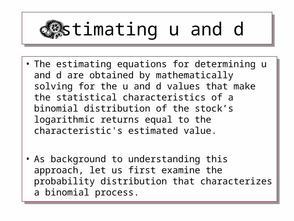
• The estimating equations for determining u and d are obtained by mathematically solving for the u and d values that make the statistical characteristics of a binomial distribution of the stock’s logarithmic returns equal to the characteristic's estimated value.
• As background to understanding this approach, let us first examine the probability distribution that characterizes a binomial process.

Binomial Process• The binomial process that we have described for spot rates
yields after n periods a distribution of n + 1possible spot rates.
• This distribution is not normally distributed because the left-side of the distribution has a limit at zero (i.e. we generally do not have negative spot rates).
• The distribution of spot rate can be converted into a distribution of logarithmic returns, gn:
0
nn S
Slng

Binomial Process
• The distribution of logarithmic returns can take on negative values and can be normally distributed if the probability of the spot rate increasing in one period (q) is .5.
• The next exhibit shows a distribution of spot rates and their corresponding logarithmic returns for the case in which u = 1.1, d = .95, and S0 = 100.

10.S0
0953.)1.1ln(g
5.p,11.S
u
11u
0513.)95ln(.g
5.p,095.S
d
10d
1906.)1.1ln(g
25.p,121.S2
uu
22uu
044.))95)(.1.1ln((g
5.p,1045.S
ud
21ud
1026.)95ln(.g
25.p,09025.S2
dd
20dd
2859.)1.1ln(g
125.p,1331.S3
uuu
33uuu
1393.))95)(.1.1ln((g
375.p,11495.S2
uud
32uud
0073.))95)(.1.1ln((g
375.p,099275.S2
udd
31udd
1539.)95ln(.g
125.p,08574.S3
ddd
30ddd
3812.)1.1ln(g
0625.p,1464.S4
uuuu
44uuuu
2346.))95)(.1.1ln((g
25.p,126445.S3
uuud
43uuud
088034.))95)(.1.1ln((g
375.p,1092025.S22
uudd
42uudd
0585697.))95)(.1.1ln((g
25.p,0943.S3
uddd
41uddd
20517.)95ln(.g
0625.p,08145.S4
dddd
40dddd
5.q,95.d,1.1u
onDistributiBinomial
)g(V
)g(E
n
n
0054.
022.
0108.
044.
0162.
066.0216.
088.

Binomial Process
• Note: When n = 1, there are two possible spot rates and logarithmic returns:
0513.)95ln(.)dln(S
dSln
095.)1.1ln()uln(S
uSln
0
0
0
0

Binomial Process
• When n = 2, there are three possible spot rates and logarithmic returns:
1026..)95ln(.)dln(S
Sdln
044.)]95)(.1.1ln[()udln(S
udSln
1906.)1.1ln()uln(S
Suln
22
0
02
0
0
22
0
02

Binomial ProcessBinomial Process
• n = 1, there are two possible rates and logarithmic returns
• n = 2, there are three possible rate and logarithmic returns
• n = 3, there are four possible rates and logarithmic returns
• n = 1, there are two possible rates and logarithmic returns
• n = 2, there are three possible rate and logarithmic returns
• n = 3, there are four possible rates and logarithmic returns

Binomial ProcessBinomial Process
• The probability of attaining any of these rates is equal to the probability of the spot rate increasing j times in n period: pnj.
• The probability of attaining any of these rates is equal to the probability of the spot rate increasing j times in n period: pnj.
jnjnj )q1(q
!j)!jn(
!np
In a binomial process,
this probability is

Binomial Distribution
• Using the binomial probabilities, the expected value and variance of the logarithmic return after one period are .022 and .0054:
0054.]022.0513.[5.]022.0953[.25.)g(V
022.)0513.(5.)0953(.5.)g(E22
1
1

Binomial Distribution
• The expected value and variance of the logarithmic return after two periods are .044 and .0108:
• The means and variances for the four distributions are shown at the bottom of the exhibit.
0108.]044.1026.[25.]044.044[.5.]044.1906[.25.)g(V
044.)1026.(25.)0440(.5.)1906(.25.)g(E222
n
n

Binomial ProcessBinomial Process
• In examining each distribution’s mean and variance, note that as the number of periods increases, the expected value and variance increase by a multiplicative factor such that:
• The parameter values (expected value and variance) after n periods are equal to the parameter values for one period time the number of periods.
)g(nV)g(V
)g(nE)g(E
1n
1n

Binomial ProcessBinomial Process
• Note: The expected value and the variance are also equal to
• Note: The expected value and the variance are also equal to
2n
n
)]d/u)[ln(q1(nq)g(V
]dln)q1(ulnq[n)g(E

Solving for u and dSolving for u and d
• Given the features of a binomial distribution, the formulas for estimating u and d are found by solving for the u and d values that make the expected value and the variance of the binomial distribution of the logarithmic return of spot rates equal to their respective estimated parameter values under the assumption that q = .5 (or equivalently that the distribution is normal).
• Given the features of a binomial distribution, the formulas for estimating u and d are found by solving for the u and d values that make the expected value and the variance of the binomial distribution of the logarithmic return of spot rates equal to their respective estimated parameter values under the assumption that q = .5 (or equivalently that the distribution is normal).

Solving for u and dSolving for u and d
• If we let e and Ve be the estimated mean and variance of the logarithmic return of spot rates for a period equal in length to n periods, then our objective is to solve for the u and d values that simultaneously satisfy the following equations:
• If we let e and Ve be the estimated mean and variance of the logarithmic return of spot rates for a period equal in length to n periods, then our objective is to solve for the u and d values that simultaneously satisfy the following equations:
e2
1
e1
V)]d/u)[ln(q1(nq)g(nV
]dln)q1(ulnq[n)g(nE

Solving for u and dSolving for u and d
• If q = .5, then the formula values for u and d that satisfy the two equations are
• If q = .5, then the formula values for u and d that satisfy the two equations are
n/en/eV
n/en/eV
ed
eu

u and d: Exampleu and d: Example
• If the estimated expected value and variance of the logarithmic return were e = .044 and Ve = .0108 for a period equal in length to n = 2, then using the above equations, u would be 1.1 and d would be .95:
• If the estimated expected value and variance of the logarithmic return were e = .044 and Ve = .0108 for a period equal in length to n = 2, then using the above equations, u would be 1.1 and d would be .95:
95.ed
1.1eu2/044.2/0108.
2/044.2/0108.

u and d for Large nu and d for Large n
• Note: In the equations for u and d, as n increases the mean term in the exponent goes to zero quicker than the square root term.
• As a result, for large n (e.g., n = 30), the mean term’s impact on u and d is negligible and u and d can be estimated as:
• Note: In the equations for u and d, as n increases the mean term in the exponent goes to zero quicker than the square root term.
• As a result, for large n (e.g., n = 30), the mean term’s impact on u and d is negligible and u and d can be estimated as:
u/1ed
eun/V
n/V
e
e

Annualized Mean and VarianceAnnualized Mean and Variance
e and Ve are the mean and variance for a length of time equal to the bond’s maturity.
• Often the annualized mean and variance are used.
• The annualized mean and variance are obtained by multiplying the estimated mean and variance of a given length (e.g., month) by the number of periods of that length in a year (e.g., 12).

Annualized Mean and VarianceAnnualized Mean and Variance
• When the annualized mean and variance are used, then these parameters must by multiplied by the proportion h, defined earlier as the time of the period being analyzed expressed as a proportion of a year, and n is not needed since h defines the length of tree’s period:
• When the annualized mean and variance are used, then these parameters must by multiplied by the proportion h, defined earlier as the time of the period being analyzed expressed as a proportion of a year, and n is not needed since h defines the length of tree’s period:
Ae
Ae
Ae
Ae
hhV
hhV
ed
eu

Annualized Mean and VarianceAnnualized Mean and Variance
• If the annualized mean and variance of the logarithmic return of one-year spot rates were .044 and .0108, and we wanted to evaluate a three-year bond with six-month periods (h = ½ of a year), then we would use a six-period tree to value the bond (n = (3 years)/(½) = 6 periods) and u and d would be 1.1 and .95:
• If the annualized mean and variance of the logarithmic return of one-year spot rates were .044 and .0108, and we wanted to evaluate a three-year bond with six-month periods (h = ½ of a year), then we would use a six-period tree to value the bond (n = (3 years)/(½) = 6 periods) and u and d would be 1.1 and .95:
95.ed
1.1eu044).2/1(0108).2/1(
044.)2/1(0108).2/1(

Annualized Mean and VarianceAnnualized Mean and Variance
• Note that the annualized standard deviation cannot be obtained simply by multiplying the quarterly standard deviation by four. Rather, one must first multiply the quarterly variance by four and then take the square root of the resulting annualized variance.
• Note that the annualized standard deviation cannot be obtained simply by multiplying the quarterly standard deviation by four. Rather, one must first multiply the quarterly variance by four and then take the square root of the resulting annualized variance.

Estimating e and Ve Estimating e and Ve
• The simplest estimate of e and Ve is the average mean and variance computed from an historical sample of spot rates (such as the rates on T-bills).
• Example: – Historical quarterly one-year spot rates over 13
quarters are shown in the next exhibit.
– The 12 logarithmic returns are calculated by taking the natural log of the ratio of spot rates in one period to the rate in the previous period (St/St-1).

Estimating e and Ve Estimating e and Ve
– From this data, the historical quarterly logarithmic mean return and variance are:
– From this data, the historical quarterly logarithmic mean return and variance are:
004209.11
046297.
11
]g[
V
012
0
12
g
12
1t
2et
e
12
1tt
e

Estimating e and Ve Estimating e and Ve
Quarter Spot Rate, St St/St-1 g t = ln(St/St-1) (gt - e)2
Y1.1
Y1.2
Y1.3
Y1.4
Y2.1
Y2.2
Y2.3
Y2.4
Y3.1
Y3.2
Y3.3
Y3.4
Y4.1
10.6%
10.0%
9.4%
8.8%
9.4%
10.0%
10.6%
10.0%
9.4%
8.8%
9.4%
10.0%
10.6%
–
.9434
.9400
.9362
1.0682
1.0638
1.0600
.9434
.9400
.9362
1.0682
1.0638
1.0600
--
-.0583
-.0619
-.0659
.0660
.0619
.0583
-.0583
-.0619
-.0660
.0660
.0619
.0583
0
e = 0
–
.003395
.003829
.004350
.004350
.003829
.003395
.003395
.003829
.004350
.004350
.003829
.003395
.046297
004209.11
046297.Vq
e

Estimating e and Ve Estimating e and Ve
0
)0(4
4
Ae
Ae
qe
Ae
016836.V
)004209(.4V
V4V
Ae
Ae
qe
Ae
Multiplying the historical quarterly mean and
variance by 4, we obtain an annualized mean
and variance, respectively, of 0 and .016836.
Estimating e and Ve Estimating e and Ve
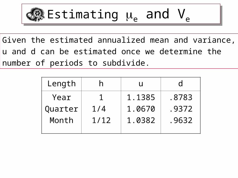
Length h u d
Year
Quarter
Month
1
1/4
1/12
1.1385
1.0670
1.0382
.8783
.9372
.9632
Given the estimated annualized mean and variance,
u and d can be estimated once we determine the
number of periods to subdivide.

FeaturesFeatures
• A binomial interest rates tree generated using the u and d estimation approach is constrained to have an end-of-the-period distribution with a mean and variance that matches the analyst’s estimated mean and variance.
• A binomial interest rates tree generated using the u and d estimation approach is constrained to have an end-of-the-period distribution with a mean and variance that matches the analyst’s estimated mean and variance.

FeaturesFeatures
• The binomial tree generated from u and d estimates is not constrained to yield a bond price that matches its equilibrium price: price obtain by discounting the bond’s cash flows by spot rates.
• As a result, analysts using such models need to make additional assumptions about the risk premium in order to explain the bond’s equilibrium price.
• In contrast, calibration models are constrained to match the current term structure of spot rates and therefore yield bond prices that are equal to their equilibrium values.

Calibration ModelCalibration Model
• The calibration model generates a binomial tree by finding spot rates that satisfy two conditions:
1. A variability condition that governs the relation between the upper and lower spot rates.
2. A price condition in which the bond value obtained from the tree is consistent with the equilibrium bond price given the current spot yield curve.

Variability ConditionVariability Condition
• In our derivation of the formulas for u and d, we assumed that the distribution of the logarithmic return of spot rates was normal.
• This assumption also implies the following relationship between the upper and lower spot rate:
• In our derivation of the formulas for u and d, we assumed that the distribution of the logarithmic return of spot rates was normal.
• This assumption also implies the following relationship between the upper and lower spot rate:
n/V2du
eeSS

Variability ConditionVariability Condition
– Given:
– Therefore:
– Given:
– Therefore:
0d
0u
dSS
uSS
d
uSS
d
SS
u
S
du
d0
u

Variability ConditionVariability Condition
– Substituting the equations for u and d, we obtain:
– Or in terms of the annualized variance:
– Substituting the equations for u and d, we obtain:
– Or in terms of the annualized variance:
n/eV2dn/en/eV
n/en/eV
du eSe
eSS
AehV2
du eSS

Variability ConditionVariability Condition
• Example: Given a lower rate of 9.5% and an annualized variance of .0054, the upper rate for a one-period binomial tree of length one year (h = 1) would be 11%:
• If the current one-year spot rate were 10%, then these upper and lower rates would be consistent with the upward and downward parameters of u = 1.1 and d = .95.
• This variability condition would therefore result in a binomial tree identical to the one shown in the earlier exhibit.
11.e%5.9S 0054.2u

Price ConditionPrice Condition
• A price condition requires that the bond value obtained from the tree is equal to the equilibrium bond price given the current spot yield curve.
• To generate a tree that satisfies the price condition requires solving for a lower spot rate that along with the variability relation yields a bond price that is equal to the equilibrium bond price.

Price ConditionPrice Condition
• Suppose the current yield curve has the following one-, two-, and three-year spot rates (yt):
• Assume the estimated annualized logarithmic mean and variance are:
• Suppose the current yield curve has the following one-, two-, and three-year spot rates (yt):
• Assume the estimated annualized logarithmic mean and variance are:
%24488.10y
%12238.10y
%10y
3
2
1
0054.V
048167.Ae
Ae

Price ConditionPrice Condition
• Using the u and d approach, a one-period tree of length one year would have up and down parameters of u = 1.12936 and d = .975:
• Given the current one-period spot rate of 10%, the tree’s possible spot rate would be Su = 11.2936% and Sd = 9.75%.
• Using the u and d approach, a one-period tree of length one year would have up and down parameters of u = 1.12936 and d = .975:
• Given the current one-period spot rate of 10%, the tree’s possible spot rate would be Su = 11.2936% and Sd = 9.75%.
975.ed
12936.1eu048167.)1(0054).1(
048167.)1(0054).1(

Price ConditionPrice Condition
• These rates, though, are not consistent with the existing term structure.
• If we value a two-year pure discount bond (PDB) with a face value of $1 using this tree, we obtain a value of .82258 that, given the two-year spot rate of 10.12238%, differs from the equilibrium price on the two-year zero discount bond of B0
M = .8246:
8246.)1012238.1(
1
)y1(
1B
82258.10.1
]0975.1/1[5.]112936.1/1[5.
S1
B5.B5.B
222
M0
0
du0

898524.112936.1
1B
112936.e0975.S
u
0054.2u
9111617.0975.1
1B
0975.S
d
d
1Buu
1Bud
1Bdd
82258.B10.1
)9111617(.5.)898524(.5.B
10.S
0
0
0
8246.)1012238.1(
1B
1012238.y
2M0
2

Price ConditionPrice Condition
• Thus, the tree generated from our estimates of u and d is not consistent with the current interest rate structure.
• Thus, the tree generated from our estimates of u and d is not consistent with the current interest rate structure.

Price ConditionPrice Condition
• To make our tree consistent with the term structure, we need to find the Sd value such that when
the value of the two-year bond obtained from the tree is equal to the current equilibrium price of a two-year zero discount bond: B0
M = .8246.
• To make our tree consistent with the term structure, we need to find the Sd value such that when
the value of the two-year bond obtained from the tree is equal to the current equilibrium price of a two-year zero discount bond: B0
M = .8246.
0054.2d
hV2du eSeSS
Ae

Price ConditionPrice Condition
• Mathematically, we need to find Sd where:
• In terms of the example: find Sd where:
• Mathematically, we need to find Sd where:
• In terms of the example: find Sd where:
0
du2
2 S1
)]S1/(1/(1[5.)]S1/(1[5.
)y1(
1
0
dhV2
d2
2 S1
)]S1/(1[5.)]eS1/(1[5.
)y1(
1Ae
0
du2
2 S1
B5.B5.
)y1(
1
10.1
)]S1/(1[5.)]eS1/(1[5.
)1012238.1(
1 d0054.2
d2

Price ConditionPrice Condition
• Solving the above equation for Sd, yields a rate of 9.5%.
• At Sd = 9.5%, we have a binomial tree of one-year spot rates of Su = 11% and Sd = 9.5% that simultaneously satisfies our variability condition and price condition.
• That is, the rate is consistent with the estimated volatility of .0054 and the current yield curve with one-year and two-year spot rates of 10% and 10.12238%

9009.)11.1(
1B
%11e095.S
u
0054.2u
8246.
)10.1(
)913242(.5.)9009(.5.B
%10S
0
0
1Buu
913242.)095.1(
1B
%5.9S
d
d
1Bud
1Bdd 8246.)1012238.1(
1
)y1(
1B
223
M0

Price ConditionPrice Condition
• The lower rate of 9.5% represents a decline from the current rate of 10%, which is what we tend to expect in a binomial process.
• This is because we have calibrated the binomial tree to a relatively flat yield curve.
• The lower rate of 9.5% represents a decline from the current rate of 10%, which is what we tend to expect in a binomial process.
• This is because we have calibrated the binomial tree to a relatively flat yield curve.

Price ConditionPrice Condition
• If we had calibrated the tree to a positively sloped yield curve, then it is possible that both rates next period could be greater than the current rate; although the upper rate will be greater than the lower.
• For example, if the current two-year spot rate were 10.5% instead of 10.12238%, then the equilibrium price of a two-year bond would be .8189 and the Sd and Su values that calibrate the tree to this price and variability of .0054 would be 10.20066% and 11.8156%.

8943.118156.1
1B
118156.e102006.S
u
0054.2u
9074.1020066.1
1B
1020066.S
d
d
1Buu
1Bud
1Bdd
8189.B10.1
)9074(.5.)8943(.5.B
10.S
0
0
0
8189.)105.1(
1B
105.y
2M0
2

Price ConditionPrice Condition
• By contrast, if we had calibrated the tree to a negatively sloped curve, then it is possible that both rates next period could be lower than the current one.
• By contrast, if we had calibrated the tree to a negatively sloped curve, then it is possible that both rates next period could be lower than the current one.

Variability Condition: Period 2Variability Condition: Period 2
• Given our estimated one-year spot rates after one period of 9.5% and 11%, we can now move to the second period and determine the tree’s three possible spot rates using a similar methodology.
• The variability condition follows the same form as the one period; that is:
• Given our estimated one-year spot rates after one period of 9.5% and 11%, we can now move to the second period and determine the tree’s three possible spot rates using a similar methodology.
• The variability condition follows the same form as the one period; that is:
Ae
Ae
Ae
hV4dd
hV2uduu
hV2ddud
eSeSS
eSS

Price Condition: Period 2Price Condition: Period 2
• The price condition requires that the binomial value of a three-year zero coupon bond be equal to the equilibrium price.
• Analogous to the one-period case, this condition is found by solving for the lower rate Sdd that, along with the above variability conditions and the rates for Su and Sd obtained previously, yields a value for a three-year zero-coupon bond that is equal to the price on a three-year zero coupon bond yielding 10.24488%.

Price Condition: Period 2Price Condition: Period 2
• Mathematically find Sdd where: • Mathematically find Sdd where:
0
du3
2 S1
B5.B5.
)y1(
1
0
d
ddud
u
uduu
32 S1
S1
B5.B5.5.
S1
B5.B5.5.
)y1(
1
10.1
095.1
)]S1/(1[5.)]eS1/(1[5.5.
11.1
)]eS1/(1[5.)]eS1/(1[5.5.
)1024488.1(
1dd
0054.2dd
0054.2dd
0054.4dd
3

Price Condition: Period 2Price Condition: Period 2
• Using an iterative (trial and error) approach, we find that a lower rate of Sdd = 9.025% yields a binomial value that is equal to the equilibrium price of the three-year bond of .7463
• Using an iterative (trial and error) approach, we find that a lower rate of Sdd = 9.025% yields a binomial value that is equal to the equilibrium price of the three-year bond of .7463

8920607.121.1
1B
%1.12e%025.9S
uu
0054.4uu
9172208.09025.1
1B
%025.9S
dd
dd
809661.11.1
)9053871(.5.)8920607(.5.B
%11S
u
u
832241.095.1
)9172208(.5.)9053871(.5.B
%5.9S
d
d
7463.10.1
)832241(.5.)809661(.5.B
%10S
0
0
1
1
1
1
9053871.1045.1
1B
%45.10e%025.9S
ud
0054.2ud
7463.)1024488.1(
1
)y1(
1B
333
M0
2-Period Binomial Tree2-Period Binomial Tree
• The two-period binomial tree is obtained by combining the upper and lower rates found for the first period with the three rates found for the second period. This yields a tree that is consistent with the estimated variability condition and with the current term structure of spot rates.
• The two-period binomial tree is obtained by combining the upper and lower rates found for the first period with the three rates found for the second period. This yields a tree that is consistent with the estimated variability condition and with the current term structure of spot rates.

%10.12SuS 02
uu
%45.10udSS 0ud
%025.9SdS 02
dd
%00.11uSS 0u
%5.9dSS 0d
%00.10S0

Growing the Binomial TreeGrowing the Binomial Tree
• To grow the tree, we continue with this same process. For example, to obtain the four rates in Period 3, we solve for the Sddd that along with the spot rates found previously for periods one and two and the variability relations, yields a value for a four-year PDB that is equal to the equilibrium price.
• To grow the tree, we continue with this same process. For example, to obtain the four rates in Period 3, we solve for the Sddd that along with the spot rates found previously for periods one and two and the variability relations, yields a value for a four-year PDB that is equal to the equilibrium price.
Valuation of Coupon BondValuation of Coupon Bond
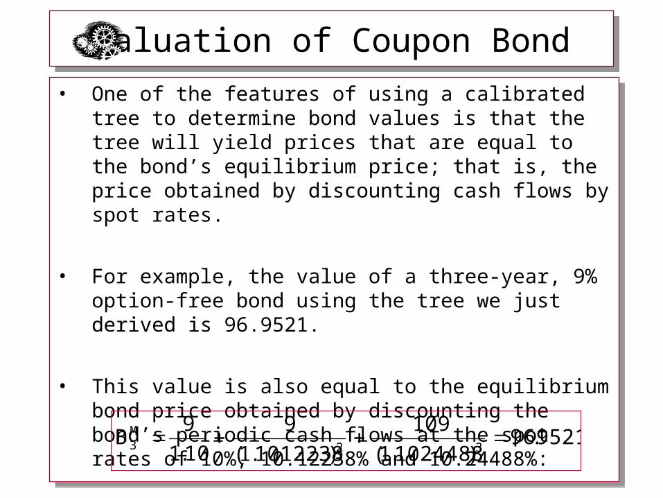
• One of the features of using a calibrated tree to determine bond values is that the tree will yield prices that are equal to the bond’s equilibrium price; that is, the price obtained by discounting cash flows by spot rates.
• For example, the value of a three-year, 9% option-free bond using the tree we just derived is 96.9521.
• This value is also equal to the equilibrium bond price obtained by discounting the bond’s periodic cash flows at the spot rates of 10%, 10.12238% and 10.24488%:
9521.96)1024488.1(
109
)1012238.1(
9
10.1
9B
32M3

2346.97121.1
109B
%1.12SuS
uu
02
uu
9771.9909025.1
109B
%025.9SdS
dd
02
dd
3612.96
)11.1(
)96872.98(5.)92346.97(5.B
%11uSS
u
0u
95.d,1.1u,10.S
100$F,9C
0
9335.98
)095.1(
)99771.99(5.)96872.96(5.B
%5.9dSS
d
0d
9521.96
)10.1(
)99335.98(5.)93612.96(5.B
%10S
0
0
109
109
109
109
6872.981045.1
109B
%45.10udSS
ud
0ud
9521.96)1024488.1(
109
)1012238.1(
9
10.1
9B
32M3

FeatureFeature
• Thus, one of the features of the calibrated tree is that it yields values on option-free bonds that are equal to the bond’s equilibrium price.
• Thus, one of the features of the calibrated tree is that it yields values on option-free bonds that are equal to the bond’s equilibrium price.

Valuation of Callable Coupon BondValuation of Callable Coupon Bond
• The primary purpose of generating the tree, though, is to value bonds with embedded options. In this example, if the three-year bond were callable at 98, then its value would be 96.2584.
• The primary purpose of generating the tree, though, is to value bonds with embedded options. In this example, if the three-year bond were callable at 98, then its value would be 96.2584.

2346.97
]98,2346.97[MinB
]CP,B[MinB
2346.97121.1
109B
%1.12SuS
Cuu
uuCuu
uu
02
uu
98
]98,9771.99[MinB
]CP,B[MinB
9771.9909025.1
109B
%025.9SdS
Cdd
ddCdd
dd
02
dd
0516.96]98,0516.96[MinB
]CP,B[MinB
0516.96
)11.1(
)9.98(5.)92346.97(5.B
%11uSS
Cu
uCu
u
0u
95.d,1.1u,10.S
98CP,100$F,9C
0
7169.97]98,7169.97[MinB
]CP,B[MinB
7169.97
)095.1(
)998(5.)998(5.B
%5.9dSS
Cd
dCd
d
0d
2584.96
)10.1(
)97169.97(5.)90516.96(5.B
%10S
C0
0
109
109
109
109
98
]98,6872.98[MinB
]CP,B[MinB
6872.981045.1
109B
%45.10udSS
Cud
udCud
ud
0ud

Option-Free FeaturesOption-Free Features
• One of the features of the calibration model is that it prices a bond equal to its equilibrium price.
• A bond’s equilibrium price is an arbitrage-free
price. That is, if the market does not price the bond at its equilibrium value, then arbitrageurs would be able to realize a riskless return either by buying the bond, stripping it into a number of zero discount bonds, and selling them, or by buying a portfolio of zero discount bonds, bundling them into a coupon bond, and selling it.

Option-Free FeaturesOption-Free Features
• In general, a security can be valued by arbitrage by pricing it to equal the value of its replicating portfolio: a portfolio constructed so that it has the same cash flows.
• The replicating portfolio of a coupon bond, in turn, is the portfolio of zero discount bonds. Thus, one of the important features of the calibration model is that it yields prices on option-free bonds that are arbitrage free.

Option-Free FeaturesOption-Free Features
• The calibration model also values a bond’s embedded options as arbitrage-free prices.
• Consider the three-year, 9% callable bond priced in terms of the calibrated binomial tree shown in the exhibit:
– The value of the call option in period 1 is .3095 when the rate is at 11%.
– The value of the call option in period 1 is 1.2166 when the rate is at 9.5%.
– The value of the option in the current period is .6937.
• Each of these values was determined by calculating the present value of each option’s expected value.
• These values are also equal to the values of their replicating portfolios.

2346.9702346.97
VBB
0IVV
0]0,982346.97[Max
]0,CPB[MaxIV
2346.97B%,1.12S
Cuu
NCuu
Cuu
Cuu
NCuu
NCuuuu
0516.963095.3612.96VBB
3095.]0,3095[.Max]IV,V[MaxV
0]0,983612.96[Max
]0,CPB[MaxIV
3095.)11.1(
)6872(.5.)0(5.V
3612.96B%,11S
Cu
NCu
Cu
HCu
NCu
H
NCuu
95.d,1.1u,10.S
98CP,100$F,9C
0
2584.96
6937.9521.96
VBB
6937.)10.1(
)2166.1(5.)3095(.5.VV
9521.96B%,10S
C0
NC0
C0
HC0
NC00
986872.6872.98
VBB
6872.IVV
6872.]0,986872.98[Max
]0,CPB[MaxIV
6872.98B%,45.10S
Cud
NCud
Cud
Cud
NCud
NCudud
989771.19771.99
VBB
9771.1IVV
9771.1]0,989771.99[Max
]0,CPB[MaxIV
9771.99B%,025.9S
Cdd
NCdd
Cdd
Cdd
NCdd
NCdddd
7169.972166.19335.98VBB
2166.1]9335.,2166.1[Max]IV,V[MaxV
9335.]0,989335.98[Max
]0,CPB[MaxIV
2166.1)095.1(
)9771.1(5.)6872(.5.V
9335.98B%,5.9S
Cd
NCd
Cd
HCd
NCd
H
NCdd

Option-Free FeaturesOption-Free Features
• The current call price of .6937 is equal to the value of a portfolio consisting of
• Next period the possible cash flows on the two-year bond are
• Next period the cash flow on the one-year bond is 109.
• The current call price of .6937 is equal to the value of a portfolio consisting of
• Next period the possible cash flows on the two-year bond are
• Next period the cash flow on the one-year bond is 109.
A one-year, 9% option-free bond and a two-year, 9% option-free bond constructed so that next year the portfolio is worth .3095 if the spot rate is 11% and 1.2166 if the rate is at 9.5%.
Bu + C = (109/1.11) + 9 = 107.198198
Bd + C = (109/1.095) + 9 = 108.543379

Option-Free FeaturesOption-Free Features
• The replicating portfolio is formed by solving for the number of one-year bonds, n1, and the number of two-year bonds, n2, where:
• Solving for n1 and n2, we obtain:
• The replicating portfolio is formed by solving for the number of one-year bonds, n1, and the number of two-year bonds, n2, where:
• Solving for n1 and n2, we obtain:
674333.0n
66035.0n
2
1
2166.1)543379.108(n)109(n
3095.)198198.107(n)109(n
21
21
Thus, a portfolio formed by buying .674333 issues of a two-year bond and shorting .66035 issues of a one-year bond will yieldpossible cash flows next year of .3095 if the spot rate is at 11%and 1.2166 if the rate is at 9.5%.

Option-Free FeaturesOption-Free Features
• Given the current one-year and two-year bond prices of 99.09091 and 98.06435, the value of this replicating portfolio is .6937:
• Given the current one-year and two-year bond prices of 99.09091 and 98.06435, the value of this replicating portfolio is .6937:
6937.)06435.98)(674333(.)09091.99)(66035.(V
06435.98)1012238.1(
9
10.1
9B
09091.9910.1
109B
RP0
22
1

Option-Free FeaturesOption-Free Features
• Since the replicating portfolio and the call option have the same cash flows, by the law of one price they must be equally priced.
• Thus, in the absence of arbitrage, the price of the call is equal to .6937, which is the same price we obtained by discounting the option’s expected value using the calibrated binomial interest rate tree.

Option-Free FeaturesOption-Free Features
• The two call values in period 1 of .3095 and 1.2166 are likewise equal to the values of their replicating portfolios.
• For example, at the 11% rate a replicating portfolio consisting of .4730827 of the two-year, 9% bond (original three-year) and -.46108027 issues of a one-year, 9% bond (original two-year bond) will yield cash flows in period 2 equal to 0 if the spot rate is 12.1% and .6872 if the rate is 10.45%.
• At that node, the price on the one-year bond is 109/1.11 = 98.198198 and the price of the two-year is 96.3612 (see exhibit).
• At these prices, the value of the replicating portfolio is
.30956 = (-.46108027)(98.198198) + (.4730827)(96.3612)
• This value matches the value of the call.

Option-Free FeaturesOption-Free Features
• At the lower node, the replicating portfolio consists of -.98165 one-year, 9% bonds priced at 99.54338 (= 109/1.095) and 1 two-year, 9% bond priced at 98.9335 (see exhibit ).
• This portfolio’s possible cash flows in period 2 match the possible call values of .6872 and 1.9771 and its period 1 value is equal to the call value of 1.2166.

Arbitrage-Free ModelArbitrage-Free Model
• With the option values equal to their replicating portfolio values, the calibration model has the feature of pricing embedded options equal to their arbitrage-free prices.
• Because of this feature and the feature of pricing option-free bonds equal to their equilibrium prices, the calibration model is referred to as an arbitrage-free model.
• This arbitrage-free feature of the calibration model is one of the main reasons that many practitioners favor this model over the equilibrium model.

Option-Adjusted SpreadOption-Adjusted Spread
• In addition to valuation, the binomial tree also can be used to estimate the option spread.
• The simplest way to estimate the option spread is to estimate the YTM for a bond with an option given the bond’s values as determined by the binomial model, then subtract that rate from the YTM of an otherwise identical option-free bond.

Option-Adjusted SpreadOption-Adjusted Spread
• Example: In the previous example the value of the three-year, 9% callable was 96.2584, while the equilibrium price of the noncallable was 96.9521. Using these prices, the YTM on the callable is 10.51832% and the YTM on the noncallable is 10.2306, yielding an option spread of .28772%:
• Example: In the previous example the value of the three-year, 9% callable was 96.2584, while the equilibrium price of the noncallable was 96.9521. Using these prices, the YTM on the callable is 10.51832% and the YTM on the noncallable is 10.2306, yielding an option spread of .28772%:
%28772.%2306.10%51832.10YTMYTMSpreadOption
%51832.10YTM
)YTM1(
109
)YTM1(
9
YTM1
92584.96:BondCallable
%2306.10YTM
)YTM1(
109
)YTM1(
9
YTM1
99521.96:BondFreeOption
NCC
C
32
NC
32

Option-Adjusted SpreadOption-Adjusted Spread
• The problem with using this approach to estimate the spread is that not all of the possible cash flows of the callable bond are considered.
• In three of the four interest rate scenarios, for example, the bond could be called, changing the cash flow pattern from three periods of 9, 9, and 109 to two periods of 9 and 107.
• An alternative approach that addresses this problem is the option-adjusted spread (OAS) analysis.

Option-Adjusted Spread AnalysisOption-Adjusted Spread Analysis
• The objective of option-adjusted spread analysis is to solve for the option spread, k, that makes the average of the present values of the bond’s cash flows from all of the possible interest rate paths equal to the bond’s market price.
• The objective of option-adjusted spread analysis is to solve for the option spread, k, that makes the average of the present values of the bond’s cash flows from all of the possible interest rate paths equal to the bond’s market price.

Option-Adjusted Spread AnalysisOption-Adjusted Spread Analysis
• The first step is to specify the cash flows and spot rates for each path.
• In the case of the three-year bond valued with a two-period binomial interest rate tree, there are four possible paths.
• The first step is to specify the cash flows and spot rates for each path.
• In the case of the three-year bond valued with a two-period binomial interest rate tree, there are four possible paths.
Path/Time
1S1
1CF
2S1
2CF
3S1
3CF
4S1
4CF
0123
.10.0950
.09025-
-9
107
.10.095
.1045-
-9
107
.10
.11.1045
-
-9
107
.10
.11.121
-
-99
109

Option-Adjusted Spread AnalysisOption-Adjusted Spread Analysis
• The next step is to determine the appropriate two-year spot rates (y2) and three-year rates (y3) to discount the cash flows.
• These rates can be found using the geometric mean and the one-year spot rates from the tree.
• The next step is to determine the appropriate two-year spot rates (y2) and three-year rates (y3) to discount the cash flows.
• These rates can be found using the geometric mean and the one-year spot rates from the tree.
095076.1)]09025.1)(095.1)(10.1[(y
097497.1)]095.1)(10.1[(y
10.y
1Path
3/13
2/12
1
099826.1]1045.1)(095.1)(10.1[(y
097497.1)]095.1)(10.1[(y
10.y
2Path
3/13
2/12
1
104826.1]1045.1)(11.1)(10.1[(y
104989.1)]11.1)(10.1[(y
10.y
3Path
3/13
2/12
1
110300.1]121.1)(11.1)(10.1[(y
104989.1)]11.1)(10.1[(y
10.y
4Path
3/13
2/12
1

Option-Adjusted Spread AnalysisOption-Adjusted Spread Analysis
• The last step is to is to solve for the k that makes the average present values of the paths equal to the callable bond’s market price, BM
0.
• The last step is to is to solve for the k that makes the average present values of the paths equal to the callable bond’s market price, BM
0.
32
22
2
M0
)k110300.1(
109
)k104989.1(
9
)k10.1(
9
)k104989.1(
109
)k10.1(
9
)k097497.1(
109
)k10.1(
9
)k097497.1(
107
)k10.1(
9
)4/1(B

Option-Adjusted Spread AnalysisOption-Adjusted Spread Analysis
• If the market price is equal to the binomial value we obtained using the calibration model, then the option spread, k, is equal to zero.
• This reflects the fact that we have calibrated the tree to the yield curve and have considered all of the possibilities.
• In practice, though, we do not expect the market price to equal the binomial value.

Option-Adjusted Spread AnalysisOption-Adjusted Spread Analysis
• If the market price is below the binomial value, then k will be positive.
• For example, if the market priced the three-period bond at 94.6097, then the OAS (k) would be 2%.
• If the market price is below the binomial value, then k will be positive.
• For example, if the market priced the three-period bond at 94.6097, then the OAS (k) would be 2%.

Option-Adjusted Spread AnalysisOption-Adjusted Spread Analysis
• Many analysts in trying to identify mispriced bonds use the option-adjusted spread approach to estimate k instead of comparing the market price with the binomial value.
• Many analysts in trying to identify mispriced bonds use the option-adjusted spread approach to estimate k instead of comparing the market price with the binomial value.

Duration and ConvexityDuration and Convexity
• Bonds with call options are sometimes said to have negative convexity, meaning that the bond’s duration moves inversely with rate changes.
• When a bond has a call option, a rate decrease can lead to an early call, which shortens the life of the bond and lowers its duration, while an interest rate increase tends to lengthen the expected life of the bond causing its duration to increase.
• Thus, the option features of a bond can have a significant impact on the bond’s duration, as well as its convexity.

Duration and ConvexityDuration and Convexity
• The duration and convexity of bonds with embedded option features can be estimated using a binomial tree and the effective duration and convexity measures defined in chapter 4:
• The duration and convexity of bonds with embedded option features can be estimated using a binomial tree and the effective duration and convexity measures defined in chapter 4:
20
0
0
)y)(B(
B2BBConvexityEffective
)y)(B(2
BBDurationEffective
where: B- = price associated with a small decrease in rates. B+ = price associated with small increase in rates.

Duration and ConvexityDuration and Convexity
The binomial tree calibrated to the yield curve can be used to estimate B0, B- and B+:
1. B0 can be defined by the current yield curve and calibrated tree.
2. B- can be estimated by allowing for a small equal decrease in each of the yield curve rates (e.g. 10 basis points) and then using the tree calibrated to the new rates to find the price.
3. B+ can be estimated in a similar way by allowing for a small equal increase in the yield curve’s rates and then estimating the bond price using the tree calibrated to these higher rates.

Black-Scholes OPMBlack-Scholes OPM
• An approximate value of the embedded option features of a bond can also be estimated using the well-known Black-Scholes Option Pricing Model (B-S OPM)) – a model commonly used in pricing options.
• An approximate value of the embedded option features of a bond can also be estimated using the well-known Black-Scholes Option Pricing Model (B-S OPM)) – a model commonly used in pricing options.

Black-Scholes OPMBlack-Scholes OPM
• The B‑S formula for determining the equilibrium price of an embedded call or put option is:
• The B‑S formula for determining the equilibrium price of an embedded call or put option is:
Tdd
T
T)5.R()X/Bln(d
))d(N1(Be))d(N1(XV
e)d(NX)d(NBV
12
2f0
1
10TR
2P0
TR210
C0
f
f

Black-Scholes OPMBlack-Scholes OPM
where:• X = call price (CP) or put price (PP) 2 = variance of the logarithmic return of bond prices = V(ln(Bn/B0)
• T = time to expiration expressed as a proportion of a year.
• Rf = continuously compounded annual risk-free rate (if simple annual rate is R, the continuously compounded rate is ln(1+R)).
• N(d) = cumulative normal probability; this probability can be looked up in a standard normal probability table or by using the following formula:
N(d) = 1 – n(d), for d < 0
N(d) = n(d), for d > 0,
where:
n(d) = 1 - .5[1 + .196854 (d) + .115194 (d)2
+ .0003444 (d)3 + .019527(d)4 ]-4
d = absolute value of d.

Black-Scholes OPMBlack-Scholes OPM
Example:
• Suppose there is a three‑year, noncallable bond with a 10% annual coupon selling at par (F = 100).
• A callable bond that is identical in all respects except for its call feature.
• Suppose the call feature gives the issuer the right to buy the bond back at any time during the bond's life at an exercise price of 115.
• Assume the risk‑free rate is 6% and a variability of = .10 on the noncallable bond's logarithmic return.

Black-Scholes OPMBlack-Scholes OPM
Example: • The callable bond should sell at 100 minus the call price.
• The call price using the Black‑Scholes model is 8.95:
Example: • The callable bond should sell at 100 minus the call price.
• The call price using the Black‑Scholes model is 8.95:
55772.)14571(.N)d(N
62519.)31892(.N)d(N
14571.310.31892.d
31892.310.
3)10(.5.06(.)115/100ln(d
95.8e)55772(.115)62519(.100V
e)d(NX)d(NBV
2
1
2
2
1
)3)(06(.C0
TR210
C0
f

Black-Scholes OPMBlack-Scholes OPM
• The price of the callable bond is 91.05:• The price of the callable bond is 91.05:
Price of Callable Bond = Price of Noncallable Bond
- Call Premium
Price of Callable Bond = 100 - 8.95 = 91.05

Black-Scholes OPMBlack-Scholes OPM
Note: The B-S OPM assumes interest rates are constant. For most bonds, though, the change in their value is due to interest rate changes. Thus, the use of the B‑S OPM in to value the call option embedded in a bond should be viewed only as an approximation.
Note: The B-S OPM assumes interest rates are constant. For most bonds, though, the change in their value is due to interest rate changes. Thus, the use of the B‑S OPM in to value the call option embedded in a bond should be viewed only as an approximation.

WebsitesWebsites
For more information on option pricing go to www.derivativesmodels.com
www.in-the-money.com
www.optioncentral.com
For more information on option pricing go to www.derivativesmodels.com
www.in-the-money.com
www.optioncentral.com