Chaos Theory and the Tragedy of the Commons

Ralph H. Abraham∗

October 7, 2014

Abstract

Complex dynamical systems models have been used (and misused) in ser-vice of the sustainability (or tragedy) of a commons. Their misuse results fromthe widespread ignorance of chaos theory. Here we consider this problem ingeneral, and study the special case of the tragedy of the oceans in detail. Wego on then to relate the mathematical model for fisheries, due to Beverton andHolt in the 1940s, to the chaos revolution that followed. Finally, a potentialrole of education in commons management is proposed, in which participativesimulation using NetLogo might be an integral part.

CONTENTS

1. Introduction2. Complex dynamical systems3. The environmental movement4. Tragedy of the commons5. Tragedy of the oceans6. Codfish chaos7. The early days of chaos theory8. The shape of the Beverton-Holt function9. Bifurcations of the Beverton and Holt iteration10. Interpretation of the response diagram11. Systems thinking12. ConclusionAppendix: Definition of a CDSReferences

∗Mathematics Department, University of California, Santa Cruz, CA USA-95064. rha@ucsc.edu,and Founding Mentor, Ross School, East Hampton, NY.

1

1. Introduction

Many of the systems within which we live, such as ecosystems, are difficult to com-prehend because their complexity strains our cognitive capacity. Mathematical mod-eling (and computer simulation) of a complex system as a complex dynamical system(CDS) is a powerful strategy to bring understanding of such complex systems withinour grasp.1 But the CDS modeling approach has been sometimes misused for mak-ing predictions, even though chaos theory has shown that CDS models are generallyincapable of making predictions.

A crucial problem in the practical world of environmental management for sustain-ability is the conundrum known as the tragedy of the commons. In this article wewill apply the CDS strategy to this problem, especially in the exemplary case of thetragedy of the oceans: overfishing.

After some math preliminaries we review the prehistory of the modern environmentalmovement, 1957-1962. Along the way we will review the parallel developments of thefisheries model in the domain of applied mathematics (Gerhardsen, 1952; Gordon,1954; Schaefer, 1957, and Beverton and Holt, 1947-53, 1957), and the pure math ofquadratic iterations (Myrberg, 1958-1965). These developments led the way to thechaos revolution (May, 1974), which is crucial to our story of the misuse of mathmodeling in the tragedy of the oceans.

We end with some suggestions for training students for stewardship of common-pool resources, using the participatory simulation feature of the NetLogo softwarepackage. The inclusion of systems theory in a school curriculum may enhance studentunderstanding of the complexity and interconnectedness of the world around us. Thisstrategy fits well into a school curriculum.2

2. Systems

A complex dynamical system is a formidable mathematical object. And yet, a simpleand intuitive approach was provided in its early history.

1We distinguish complex systems, as found in nature, from complex dynamical systems, whichare mathematical models for complex systems. Technical definition are relegated to a appendix.

2This has been abundantly proven at the Ross School of East Hampton, NY.

2

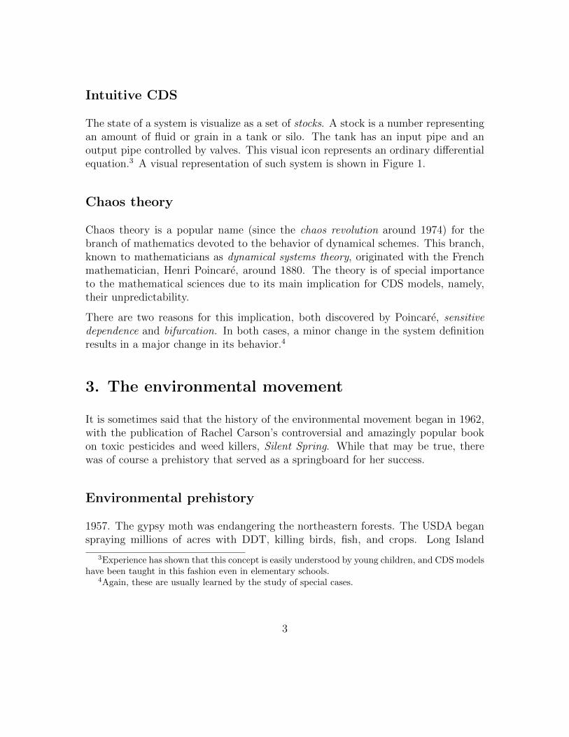
Intuitive CDS

The state of a system is visualize as a set of stocks. A stock is a number representingan amount of fluid or grain in a tank or silo. The tank has an input pipe and anoutput pipe controlled by valves. This visual icon represents an ordinary differentialequation.3 A visual representation of such system is shown in Figure 1.

Chaos theory

Chaos theory is a popular name (since the chaos revolution around 1974) for thebranch of mathematics devoted to the behavior of dynamical schemes. This branch,known to mathematicians as dynamical systems theory, originated with the Frenchmathematician, Henri Poincare, around 1880. The theory is of special importanceto the mathematical sciences due to its main implication for CDS models, namely,their unpredictability.

There are two reasons for this implication, both discovered by Poincare, sensitivedependence and bifurcation. In both cases, a minor change in the system definitionresults in a major change in its behavior.4

3. The environmental movement

It is sometimes said that the history of the environmental movement began in 1962,with the publication of Rachel Carson’s controversial and amazingly popular bookon toxic pesticides and weed killers, Silent Spring. While that may be true, therewas of course a prehistory that served as a springboard for her success.

Environmental prehistory

1957. The gypsy moth was endangering the northeastern forests. The USDA beganspraying millions of acres with DDT, killing birds, fish, and crops. Long Island

3Experience has shown that this concept is easily understood by young children, and CDS modelshave been taught in this fashion even in elementary schools.

4Again, these are usually learned by the study of special cases.

3

residents filed a suit, which was denied.5

1958. Fire ants in the American South were annoying farmers. The USDA beganseeding millions of acres with pesticide pellets more toxic than DDT.

1959. The Secretary of Health, Education and Welfare announced that some LongIsland cranberries were contaminated with aminotriazole, a weed killer thought tocause cancer, and had to be withdrawn from the market.

1961. Thalidomide, a sleeping pill supposed to be safe for pregnant women, waswithdrawn from the market after it was implicated in a rash of birth defects.

Rachel Carson

Rachel Carson (1907-1964) was born in Springdale, PA during the height of theUS movement for women’s’ suffrage. Always interested in writing and nature, sheswitched from writing to biology in college, and earned a masters degree in zoologyin 1932. Her thesis was a study of the larvae of catfish. She worked in the US Bureauof Fisheries from 1935. Her first sea story, Undersea, was published in The AtlanticMonthly of September, 1937.6 There, in a scant eight pages, we are conducted ona guided tour of the whole watery system, including food chains, sensations, andthe interconnection of all living things. The phenomenal literary style and beautyof these pages contributed to the success of the piece. In its final paragraph, sheconcludes:

Thus we see the parts of the plan fall into place: the water receiv-ing from earth and air the simple materials, storing them up until thegathering energy of the spring sun wakens the sleeping plants to a burstof dynamic activity, hungry swarms of planktonic animals growing andmultiplying upon the abundant plants, and themselves falling prey tothe shoals of fish; all, in the end, to be redissolved into their componentsubstances when the inexorable laws of the sea demand it.

This success urged her on to write a trio of books on the sea – Under the Sea Wind;a Naturalist’s Picture of Ocean Life (1941), The Sea Around Us (1951), and TheEdge of the Sea (1955) – which became best-sellers. The success of The Sea Around

5(Gartner, 1983; p. 86)6Reprinted in (Brooks, 1972; ch. 3, pp. 22-29).

4

Us made her a literary celebrity, and she resigned from the Bureau of Fisheries in1952.

In January 1958, at the height of the DDT battle on Long Island, Rachel Carsonheard from her friend Olga Owens Huckins that the birds in her private refuge weredying from the DDT spraying. This set her on a two-year path of research and writingthat culminated in the publication of Silent Spring in 1962, and the consequentexplosion of the environmental movement. Suffering poor health all her life, shelearned in 1960 that she had cancer, and ironically, finished her argument that DDTcontributed to cancer as she was dying of the disease. She lived to see the advanceof anti-pesticide legislation, received many honors, and passed away in 1964 at age56.

Her early love of the birds and the sea lead directly to the regulation of pesticides onland. Like vertebrates, environmental sensitivity evolved from the sea to land, fromfish to birds.

Silent Spring begins with a fable, in which she continues the strongly poetic voice ofher sea trilogy. Some excerpts:

I. A Fable for TomorrowThere once was a town in the heart of America where all life seemed

to live in harmony with its surroundings. The town lay in the midst ofa checkerboard of prosperous farms, with fields of grain and hillsides oforchards where, in spring, white clouds of bloom drifted above the greenfields. In autumn, oak and maple and birch set up a blaze of color thatflamed and flickered across a backdrop of pines. Then foxes barked in thehills and deer silently crossed the fields, half hidden in the mists of thefall mornings.

.....Then a strange blight crept over the area and everything began to

change. Some evil spell had settled on the community: mysterious mal-adies swept the flocks of chickens; the cattle and sheep sickened and died.Everywhere was a shadow of death.

.........In the gutters under the eaves and between the shingles of the roofs,

a white granular powder still showed a few patches; some weeks before ithad fallen like snow upon the roofs and the lawns, the fields and streams.

No witchcraft, no enemy action had silenced the rebirth of new life inthis stricken world. The people had done it themselves.

5

........What has already silenced the voices of spring in countless towns in

America? This book is an attempt to explain.

Following this poetic transition, she immediately changes her tone to a coldly scien-tific report, almost a legal brief, on the pollution of the oceans.

Due to her untimely demise, she missed the rapid evolution of the environmentalmovement around the world, and global condemnation of chemical pesticides, thatshe had spawned. Nevertheless, toxins are still seeping into the hydrosphere, wherethey will remain for centuries.

Toxins in the sea today

In Silent Spring, Rachel Carson argued against chemical pesticides, and promotedintegrated pest management as an alternative. One of her primary concerns wasDDT. Its use on land leads to contamination of the oceans, the entire food chain ofthe sea, and through the fishing industry, to the human population at the top of thechain. Where does this stand today? According to Sea Web,7

It is estimated that over 70,000 chemicals are currently in commonuse as industrial compounds, pesticides, pharmaceuticals, food additives,and other purposes, and that this number is increasing by approximately1,000 each year. Of particular concern to the health of marine mammalpopulations are the halogenated hydrocarbons (HHCs) such as the PCBs,DDT, chlordane, dioxins and furans, and the chlorinated and brominateddiphenyl ethers. Other chemical groups of concern include trace metalssuch as mercury and cadmium, organometals such as tributyltin, poly-cyclic aromatic hydrocarbons (PAHs), and radionuclides. Those coastalpopulations near intensive agriculture operations may be exposed to pe-riodic pulses of carbamate and organophosphate pesticides.

We also have to consider the increasing concentrations of such chemicals as Prozak,Roundup, antibiotics, and CO2, as well as oil, sewage, noise pollution, and plasticdebris. More information may be found online, for example, at Ocean Health Index8

and Blue Voice.9 The latter provides a list of the twelve worst Persistant Organic

7www.seaweb.org/resources/briefings/chempol mammal.php8www.oceanhealthindex.org/9www.bluevoice.org/pdf/POPsFactSheet.pdf

6

Pollutants (POPs), including DDT, PCBs, and Dioxins.

4. Tragedy of the commons

A commons, also known as a common resource or common pool resource (CPR) is aresource shared by a community of people or agencies that exploit it for gain. Thus,a commons is a complex system composing a resource (CPR) and its exploiters.

Examples

Here are some exemplary commons of current interest.

1. Atmosphere (Climate, Energy)

2. Hydrosphere (Oceans, Aquafers, Rivers)

3. Terrasphere (Topsoil, Minerals, Beaches)

4. Biosphere (Forests, Savannas, Flora, Fauna, Fisheries)

5. Infrastructure (Networks, Electromagnetic fields)

Sustainability

A problem of sustainability arises if agents over-exploit the common pool resource,taking more than it can replenish by its natural functions. While this problem hasbeen known since ancient times, it became a topic of academic discourse and researchafter the appearance in 1968 of an article by Garrett Hardin. It’s title, The tragedyof the commons, gave a new name to the problem, as well as a pessimistic theory. Forin Hardin’s view, human greed would always lead to the destruction of the commons,that is the tragedy. From its abstract:

The tragedy of the commons develops in this way. Picture a pastureopen to all. It is to be expected that each herdsman will try to keep asmany cattle as possible on the commons. Such an arrangement may workreasonably satisfactorily for centuries because tribal wars, poaching, anddisease keep the numbers of both man and beast well below the carryingcapacity of the land. Finally, however, comes the day of reckoning, that

7

is, the day when the long-desired goal of social stability becomes a reality.At this point, the inherent logic of the commons remorselessly generatestragedy.

In the ensuing debates, a positive outcome was proposed, called the comedy of thecommons, and thus evolved a whole spectrum of cases, called the drama of the com-mons. And this in fact is the title of an important book of 2002, in which theinterdisciplinary field of commons studies, rapidly expanding since 1968, is summa-rized.10 An introductory section provides an excellent history of commons studies.11

The particular commons most frequently encountered in this literature are forests,agricultural fields, and fisheries. In these contexts, the tragedies are over-cutting,over-grazing, and over-fishing, respectively.

A formal theory of the commons preceded Hardin. An influential model of a fisherydue to H. S. Gordon (1954) and M. B. Schaefer (1957) is summarized in Figure 6.12

By the way, this image is suggestively similar to that of the logistic function, an iconof chaos theory since 1958.13 More about this below.

The drama of the commons owes much to the pioneering work of the late politicaleconomist Elinor Ostrom, winner of a Swedish Bank Prize in Economics in 2009.She had faith in human nature to resolve the problem of sharing a common poolresource by spontaneously evolved agreements, called institutions, for sustainablemanagement. She supported her ideas with extensive field work in actual commonsin Africa and Nepal, and identified eight design principles for commons managementinstitutions.

5. Tragedy of the oceans

We consider now an exemplary case of CPR mismanagement, the tragedy of theoceans. The oceans comprise the largest and most complex CPR on earth, includingits water, living systems such as coral reefs, zooplankton, fishes of all sizes up to tuna,as well as sharks and marine mammals such as whales. Preying upon these systemsare huge fleets of commercial fishing boats, some almost as large as aircraft carriers,

10(Ostrom, 2002)11(Dietz, 2002).12See (Dietz, 2002; p. 9-10). Also, (Gordon, 1954) contains a reference to (Gerhardsen, 1952),

which may be the original source of this model.13See (Myrberg, 1958-1965) and (Mira, 1987; ch. 3).

8

as well as millions of sport fishers world-wide. They remove from the oceans billionsof fish and millions of metric tons of fish (the catch) every year, while egg producingfish try in vain to replenish the loss annually. As the larger fish are decimated, thefishers concentrate on smaller fish.

Fishery defined

Here are some definitions of fishery from the expert literature.14

• A stock or stocks of fish and the enterprises that have the potential of exploitingthem. (Anderson, 1977)

• A socioeconomic technological system in interaction with a marine ecosystem.(Spochr, 1980)

• Activities through which people link themselves with aquatic environments andrenewable resources. (Anderson. 1982)

Thus, a fishery is a complex dynamical system consisting of two things, fish andhumans, as a predator-prey system: fish as prey; humans as predators. Thus humansare at the top of a food chain, which is conventionally divided into discrete links,called trophic levels.

Trophic levels

Fisheries are understood in terms of these levels. The biggest predators on top, withthe small fry on the bottom. These are the levels in the language that fisheriesscientists use for the sea.

• Level 5: including humans, marine mammals

• Level 4: large carnivores, predatory fish

• Level 3: small carnivores, fish

• Level 2: herbivores, jellyfish, herring, smelt, mollusks

• Level 1: plants, zooplankton

The large predators include:

14See (McGoodwin, 1990; p. 65).

9

• Sharks

• Tuna, billfish (swordfish, marlin, sailfish)

• Cod, halibut, groupers, sea bass

• Salmon

The large predators are prized for sport fishing as well as commercial (food) fishing.Overfishing leads to declining populations of these levels.

The declining catch

For a given fish, the catch refers to that total mass – usually measured in thousandsor millions of tonnes (metric tons) – of fish caught and taken ashore, to home orto market. The by-catch is the mass of fish killed in the fishing process and thrownoverboard. Fishing effort refers to the magnitude of the collective fishing process,measured by the total number of hours of fishing, including all fishing vessels, nor-malized to a standard size and type of gear.15 According to fishery scientists, oceanstocks of large fish are declining, and some species are in danger of collapse, that is,extinction or near-extinction. Catch sizes are declining despite ever-increasing effort.In Figure 2 we see a graph of declining catch versus time for large North Atlanticpredators from 1950 to 2000.16 This also shows the rising rate of fish mortality (catchplus by-catch) as a percentage of total fish stocks per year.

In Figure 3 we see the catch for some individual species, increasing in parallel from1950 to about,1977, then declining. Note the especially precipitous decline of theNorth Atlantic cod fishery. It collapsed actually, in 1992.17 The politics of thiscollapse will be discussed in the next section.

The declining trophic level

As the larger fish are generally more valuable, their numbers and weight declineearlier, and the fishery becomes concentrated on a lower trophic level. This progres-

15(Beverton and Holt, 2004; pp. 29-33).16See the graph in (Pauly and Maclean, 2003; fig. 10). A similar plot in (Palumbi and Sotka,

2011; p. 90) shows the earlier collapse of the sardine industry in Monterey Bay, California, in 1946.At the time, this was the largest commercial fishery in the world.

17(Pauly and Maclean, 2003; fig. 6)

10

sion, known as fishing down, is shown graphically in Figure 4. Here, fishing down isdepicted on both sides of the North Atlantic, from 1950 to 1998.18

6. Codfish chaos

The collapse of the North Atlantic cod fishery in 1992 provided a significant shockto fishery management agencies worldwide. Its analysis reveals major problems inmanagement politics, which are important to other fisheries, especially those of tunaand salmon.19

One of these major problems involves the misuse of mathematical models to intim-idate and obfuscate those who are uninformed regarding the implications of chaostheory. We begin our fishy tale with the politics, following (Pilkey and Pilkey-Jarvis,2007). Then we will examine the mathematical model of (Beverton and Holt, 1957),in relation to its contemporary chaos theory in some detail.

The politics of decline

Orrin H. Pilkey (b. 1934) was Professor of Earth and Ocean Sciences at Duke Uni-versity, and Founding Director of the Program for the Study of Developed Shorelines(PSDS). He was a master of the dynamics of shoreline movements due to coastalprocesses. He pioneered the understanding of the weaknesses of the mathematicalmodels used in coastal geology.

The book, Useless Arithmetic: Why Environmental Scientists Can’t Predict the Fu-ture. written by Pilkey and his daughter Linda Pilkey-Jarvis, a geologist in the Stateof Washington’s Department of Ecology, is devoted to a number of cases in whichmathematical models are abused by politicians to mislead the public and legislators,including the collapse of the cod fishery, the safety of nuclear material stored in YuccaMountain, the rising sea level, toxicity from abandoned mines, and plant invasions.The cod collapse of 1992 is described in detail in the first chapter. Regarding thisthey have said:

One example from our book is the ”fig leaf” coverage provided byquantitative modeling in the Grand Banks fishery. The Canadian Grand

18(Pauly and Maclean, 2003; fig. 15)19See (Safina, 1998) and (Clover, 2004/2006) for these.

11

Banks fishery has been described as the greatest in the world. It providedcod to the Western world for 500 years. In our lifetime, we watched thewild and senseless overfishing lead to the demise of an industry thatemployed as many as 40,000 people. The models, which many realizedwere questionable, provided a fig leaf behind which politicians could hideto avoid making the unthinkable decision to halt fishing.20

We move on now to an oft-misused model for a fishery, and its evolution in par-allel with that of chaos theory. This fishery model, originally due to Bevertonand Holt in the interval, 1947-1953, was reported in the book (Beverton and Holt,1957/1993/2004), still in print and much used by fishery scientists. Its cover, shownin Figure 5, features the graph of their key equation, to which we now turn.

Definition of the fishery model

The dynamic model of Beverton and Holt consists of the iteration of a one-dimensionalfunction. Its graph is highly reminiscent of the logistic function much studied in chaostheory since 1954. They give some credit to Michael Graham, director of the Fish-eries Research laboratory at Lowestoft, 1945-1958.21 Figure 6 shows a prequel of thekey graph, from (Gordon, 1954) and (Schaefer, 1957). This graph shows the catch(here called landings, L) and the cost (C) as functions of effort (E), all supposed tobe totals for a given fishing fleet for an entire season.

We must pause here to give definitions of the basic variables, according to Bevertonand Holt. The fleet may consist of vessels of different size, speed, fuel usage, gear,and so on. The catch of a vessel or fleet is the total weight of fish caught and takenashore. This is sometimes indicated by YW , the yield by weight, in contrast to YN ,the yield by number.

Each vessel is to be assigned a factor called its fishing power, PF , the catch per unitfishing time, relative to a standard vessel. The fishing effort of a fleet, F , is thetotal hours of fishing time for the whole fleet, measured in standard vessels, for ayear.

The basic equation and key graph of Beverton and Holt, the foundation of theirdiscrete dynamical model, is shown in Figure 7. Here three cases are shown. In each

20Found online at https://cup.columbia.edu/static/Interview-pilkey-orrin, September 2014).21See (Graham, 1952). The papers (Gerhardsen, 1952) and (Gordon, 1954) also belong to the

early literature of this model.

12

case, the upper part shows the graph of the basic function, and below, a time seriesof values obtained by iteration, as we shall explain.

The basic function here shows recruitment, R, as a function of egg production, E.Both R and E are measured in numbers of individual fish and eggs, respectively.

The reproductive cycle of a fish begins with egg production (spawning) by a maturefish. The eggs settle to the bottom, produce larvae, which feed on zooplankton, andhang out in a nursery area. This is called the pre-recruitment phase. At a certainage (or time) t, all surviving members of this brood or year-class enter the region inwhich capture may take place. This is called recruitment, and the number enteringthis post-recruitment phase is denoted, R. Somewhat later, at time t′, a marginallyreduced number, R′, become eligible for capture. This is the exploited phase. Anatural mortality is assumed with exponential rate of decline, M .

The recruitment, as determined by egg-production and growth in the function R(E),is depicted in Figure 7. The nonlinearity of this function, shown by its single-humpedgraph, is due to the inclusion of a nonlinear density-dependent growth function dueto von Bertalanffy, The basic equation, ascribed to (Becking, 1946), is the compoundexponential 22

R(E) = αEe−βE

where α and β are positive constants. This is very similar to the iteration studied in(May and Oster, 1976).23

Iteration of the fishery model

The iteration of this discrete dynamical system is obtained by assuming a constantegg production from each individual in the post-recruitment phase. This constant isshown as the diagonal line labelled γ in the upper graphs. This is the line throughthe origin, (0, 0), with slope 1/γ.

Each year sees recruitment, eggs, and growth. Next year, new recruitment, new eggs.new growth, and so on. The three graphs differ only in the slope of the γ line, whichvaries among the three cases, decreasing from left to right.

22See (Beverton and Holt, 2004; eqn. 6.16, p. 56).23See Fig. 4 on P. 578.

13

The iteration of the discrete dynamical system goes like this.24 Our explanationrefers to the enlargement of the graph in the upper left corner of Figure 7, which isshown in Figure 8.

The red point labeled fp, at the intersection of the humped curve and the diagonalline, is a fixed point of the process. Its coordinates are (E0, R0).

Now choose a starting value for egg production, E1, at time, t0. This would havebeen the egg production of an initial recruitment, R1. This event is represented inour figure by the blue point labelled a, with coordinates (E1, R1), which is on thediagonal line directly above the value E1 on the horizontal (E) coordinate axis.

After an epoch (∆, the duration of the growth phase from eggs into recruits) weobtain a new recruitment, R2 = R(E1), at time, t1 = t0 + ∆. This is representedin Figure 8 by the blue point labelled b, with coordinates (E1, R2), which is onthe humped curve directly above the point, a. At this time, there is a new eggproduction, E2 = γR2. This is presented in Figure 8 by the blue point labelled c,with coordinates (E2, R2), which is again on the diagonal line.

We may think of our dynamic operating in two steps, in which the point a on thediagonal moves to the point c also on the diagonal. The two steps are: vertical tothe humped graph at b, then horizontal to the diagonal.

After another epoch, a recruitment R3 = R(E2) is produced at time t2 = t0 + 2∆,and so on. Thus:

• The point a = (E1R1) is on the diagonal, the graph of the linear function,E → E/γ.

• The point b = (E1, R2) is on the humped curve, the graph of the function,E → R(E).

• The point c = (E2, R2) is on the diagonal line.

• The sequence of points, a, b, c, . . ., define the cobweb of horizontal and verticalline segments in the upper three plots of Figure 7.

• The sequence of points (R1, t0), (R2, t1), . . ., define the solid lines in the lowerplots of Figure 7.

• The sequence of points (E1, t0), (E2, t1), . . ., define the dashed lines in the lowerplots of Figure 7.

24(Beverton and Holt, 2004; p. 52)

14

Beneath the key graph in each case, the time series showing R and E as functions oftime exhibits, respectively, static, periodic, and chaotic behavior. In the first case,the fixed point, fp, is an attractor, the cobweb converges to it.

Bifurcations of the Berverton and Holt model

Note that the decline of the egg-production rate per fish, γ, is the bifurcation param-eter, creating the changes in behavior from fixed, to periodic, to chaotic behavior.This parameter, for fish in the ocean, is highly sensitive to environmental factorsthat are unpredictable. Hence, the predictions of the model are highly unreliable,according to chaos theory.

Note that if the egg-production, γ, decreases, the diagonal line, having slope 1/γ,becomes steeper, and the attractive fixed point moves to the left. At a certain criticalvalue of egg-production, this fixed point arrives at the origin. This represents thedeath of the fishery. It occurs when γ = 1/α, the reciprocal of the lead coefficient ofthe compound exponential Becking equation above. This parameter represents thesurvival rate of larvae into recruits.

On the other hand, as γ increases, the diagonal line drops, and the fixed point movesto the right. Eventually, we will find the period doubling sequence leading to chaoticbehavior. This is characteristic of a healthy fishery.

This is the basic setup of chaos theory, as it developed for the iteration of one-dimensional functions, from 1954 in the work of Myrberg.25 Understandably, thiswork would not be known to Beverton and Holt during their evolution of the fisherymodel. But a generation later, we have experienced the chaos revolution following thepublications of (May, 1974) and (Li and Yorke, 1975). May, a theoretical ecologist,mentions population models even in the title of his 1974 paper. And this becomeseven more explicit in the joint paper (May and Oster, 1976). The graph of thefunction studied therein is shown in Figure 9. Note the similarity to Beverton andHolt, shown in Figure 5.

But in the work of May and Oster, the full paraphernalia of chaos theory is appliedto the model. So it seems that fisheries scientists should be well aware of the chaoticbehavior of their fundamental model well before the demise of the North Atlanticcod fishery in 1992.

25See the wonderful exposition of this work in (Mira, 1987; Ch. 3.).

15

7. The early days of chaos theory, 1959-1974

In The Chaos Avant-Garde a scheme for the history of chaos theory was proposed,based on the idea that chaos theory began with a revolution, the ”chaos revolution”,in which the word ”chaos” was attached to the branch of mathematics known as dy-namical systems theory, as a popular name. All the prior background, from Poincareup to this historical bifurcation, is regarded there as the prehistory of chaos theory,also known as ”the early days of chaos theory.” The book comprises the memoriesof the pioneers of the early days, beginning with Steve Smale in 1959.26 One of theearly threads of chaos theory concerns the iteration of a one-dimensional function,as above.27

The chaos revolution

This bifurcation moment is placed in early 1974 by Li and Yorke:

Each academic year, the Math Department of the University of Mary-land routinely organized a special year program. The topic of the programfor the academic year of 1973-74 was mathematical biology. Robert May,who was trained as a physicist but had become a professor of biology atPrinceton University, was one of the distinguished invited speakers of theprogram. During his visit in the first week of May, 1974, Professor Maydelivered five lectures, one per day. The subject of his fifth talk was theLogistic Model,

Ta(x) = ax(1− x), x ∈ [0, 1], a ∈ [0, 4]

He described his discovery, the now well-known doubling period bifurca-tions as a varies. He did not know what happened in the chaotic region,the region beyond the main cascade of period doubling! . . .

In the summer of 1974, Professor R. May was invited to give talksby many institutions in different countries of Europe. He adopted ouruse of ”chaos” as a mathematical term, and Period three implies chaostherefore began to attract considerable worldwide attention by his strongadvocacy in talks and papers.28

26See the preface in (Abraham and Ueda, 2000).27The several texts of Robert Devaney provide elementary explanations.28See (Li and Yorke, 2000; pp. 204-205).

16

The work of Myrberg

At that time, in 1974, these pioneers did not know of the earlier work of P. J. Myrbergof Helsinki, who published much of what is known today of the logistic map familyin a series of six papers in German and French, in the interval 1958 to 1963.29 By1976, May was crediting the priority of Myrberg’s papers of 1958 and 1963.30

The results of Myrberg concern the periodic attractors of the logistic family ofquadratic real mappings, and their convergent cascade to a limit point in the pa-rameter interval (see a in the equation above), beyond which the chaotic behavior ofthe model was discovered later, perhaps by Metropolsky, Stein and Stein in 1973. Inany case, the bifurcation cascade was known to May, and independently to Li andYorke, in early 1974. And the chaotic behavior was known to Li and Yorke, andcommunicated by them to May, in 1974.

8. The shape of the Beverton-Holt function

The function,

f(x) = αxe−βx

where α and β are positive constants, and x represents the current fecundity of thefish (average annual egg production per fish).31

So given a time t0, an increment ∆t (e.g., equal to one year), and the time sequence,{t0, t1 = t0+∆t, t2 = t0+2∆t, , . . .}, we have a corresponding sequence of egg counts,{E0, E1, . . .}, with E1 = f(E0), and so on. This is the basic iteration of Bevertonand Holt, which we now wish to study.

First, we consider the graph of this function, restricted to the unit interval, [0, 1].From the first derivative,

f ′(x) = α(1− βx)e−βx

29The results of Myrberg are covered in detail in (Mira, 1987; Ch. 3), including the rediscoveryin part by Metropolsky, Stein and Stein in 1973, and by Milnor and Thurston, 1977, and others.

30(May, 1976)31(Beverton and Holt, 1957; p. 56)

17

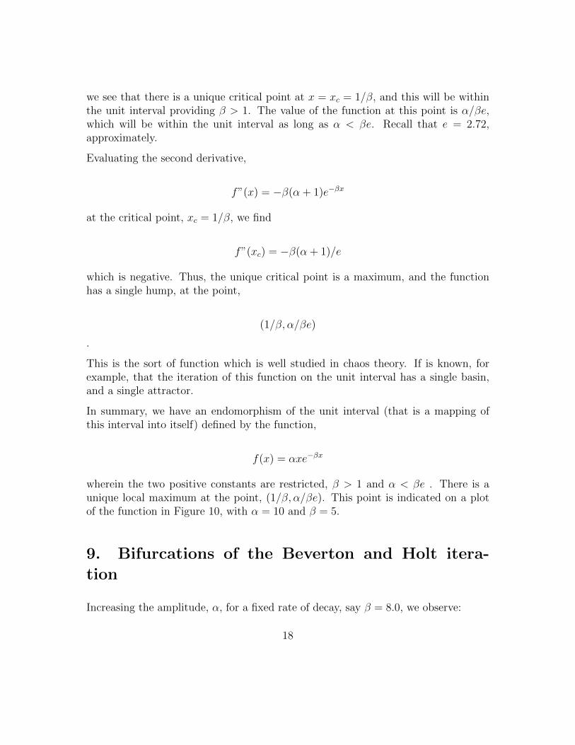
we see that there is a unique critical point at x = xc = 1/β, and this will be withinthe unit interval providing β > 1. The value of the function at this point is α/βe,which will be within the unit interval as long as α < βe. Recall that e = 2.72,approximately.

Evaluating the second derivative,

f”(x) = −β(α + 1)e−βx

at the critical point, xc = 1/β, we find

f”(xc) = −β(α + 1)/e

which is negative. Thus, the unique critical point is a maximum, and the functionhas a single hump, at the point,

(1/β, α/βe)

.

This is the sort of function which is well studied in chaos theory. If is known, forexample, that the iteration of this function on the unit interval has a single basin,and a single attractor.

In summary, we have an endomorphism of the unit interval (that is a mapping ofthis interval into itself) defined by the function,

f(x) = αxe−βx

wherein the two positive constants are restricted, β > 1 and α < βe . There is aunique local maximum at the point, (1/β, α/βe). This point is indicated on a plotof the function in Figure 10, with α = 10 and β = 5.

9. Bifurcations of the Beverton and Holt itera-

tion

Increasing the amplitude, α, for a fixed rate of decay, say β = 8.0, we observe:

18

• first a fixed point attractor, with α = 6.0, shown in Figure 11,

• then a two-periodic attractor, with α = 9.0, Figure 12,

• and a period doubling sequence leading to chaos, with α = 15.0, Figure 13,

all shown for β = 5. A full sequence is shown in the response diagram, Figure 14, asα is increased from 0 to 20 and β = 8.0.32

Here the periodic doubling sequence, familiar from the much studied logistic system,leads to chaos around α = 14. Note the prominent five-periodic window aroundα = 18.5.

10. Interpretation of the response diagram

Regarding the relation between the model data and real fish data, compare therecruitment of North Sea haddock (the main focus of Berton and Hold in the 1950s)show in Figure 15 (dashed line) with the model data of Beverton and Holt (lowerright of Fig. 7, solid line). The similarity is striking. Note that the variation defieslinear thinking, in that prior to the overfishing of the 1990s, recruitment jumps fromone extreme to the other are typical.

Our amplitude coefficient, α, is a combination of the two factors, α′ and γ, in theoriginal equation of Beverton and Holt, where α′ is a fixed constant, and γ is therelative fecundity, or average egg production of a single fish in some units. That is,α = α′γ. Thus if we follow the behavior of the unique attractor as γ decreases froma healthy value of γ = 20 down to γ = 0, we observe the behavior declining fromchaotic behavior over a full range of total egg populations, to a fixed-point attractordeclining to zero (collapse of the fishery).

Further, as γ declines, the complexity declines as well. First healthy chaos, thenworrisome periodicity, and finally stasis, declining to zero. This is evident in theBerverton-Holt model, Figure 7, in real data, Figure 15.

According to Carl Safina (1998; p. 355),

Overfishing not only directly depletes fish, it can rob other fish offood, lowering overall abundance across many species. Fishing can leadto shifts in the community, rearranging the neighborhood by pulling out

32This may be regarded as an extension of Fig. 8 in (May and Oster, 1976).

19

key species, causing cascading effects as the rest of the species adjust.This is called ”ecosystem overfishing.”

This is supported by the ”fishing down” data, showing declining trophic levels ofthe annual catch, Figure 4. Complexity, and thus sustainabiity, of the entire oceanecosystem at large, is on the way down.

We have seen that the earliest application of chaos theory, in the case of one-dimensional iterations, began in the interval 1947-1953, in the fishery model of theapplied mathematicians Beverton and Holt, working at the Fisheries Research Lab-oratory in Lowestoft, on the North Sea coast, north-east of London. Meanwhile, thepure mathematics of this field was undergoing independent development by Myrbergin Helsinki, about 1000 miles away.

Beverton and Holt were aware of the bifurcations of the model from point attractor,to periodic attractor, and ultimately to chaotic attractor. Yet it was up to Myrbergto map out the full bifurcation sequence of the model for the first time, includingthe cascade of period doubling bifurcations in the runup to chaos.

It is understandable that the full implications of chaos theory were unknown to theearly workers in fisheries science. But by the time of (May, 1974) and (May andOster, 1976), there was really no excuse. So the use of this model for setting thetotal allowable catch (TAC) for fisheries at risk of collapse, which was (and continuesto be) the case for the cod and tuna fisheries in the North Atlantic, must be due toinexcusable ignorance (or duplicity) on the part of the scientists and/or the politiciansinvolved.

11. Systems thinking

Part of the problem here is the widespread ignorance – on the part of all the actorsin the drama of the commons – of the basic concepts of complex dynamical systemstheory. This might be remedied by changes in our school curriculum. adding anextensive thread on systems thinking.

Another part of the dilemma concerns the state of morals in our global culture. Agiant bluefin tuna, its catch forbidden by law, might be worth $180,000 in Tokyo.33

What to do? This is a strong case of markets versus morals. Mathematical economistDaniel Friedman, in his excellent book, Morals and Markets, devotes a chapter to

33See (Safina, 1998; p. 114).

20

”Environmental markets and morals,” in which the North Atlantic cod collapse of1992 is carefully analyzed. While we might hope for morals to be improved in oureducational system, Friedman concludes:

The point should now be clear. Environmentalists were naive to be-lieve that a moral crusade will, by itself, secure a sound and durableenvironmental policy. Laws may be passed and bureaucracies built, butinevitably, they will be eroded when they conflict with market impera-tives.34

A system dynamics model for the tragedy of the commons is included in the NetLogoModel Library that is freely distributed along with the NetLogo computer languagesystem. This model runs in participatory simulation mode (using a NetLogo featurecalled HubNet) in which students with laptops may participate in a simulation of themanagement of a commons. A screen shot of this model is shown in Figure 16.

A more realistic and informative model might be built upon the NetLogo model,be enclosing it within a larger system, combining the commons with political andenvironmental-activist nodes. Such a scheme is indicated in Figure 17.

12. Conclusion

The plight of the ocean ecosystem is a classic example of the tragedy of the commons.The best hope for recovery seems to be conservation institutions made by localinterest groups. The development of those agreements require new levels of morality,which are difficult to create, and/or new levels of understanding of ecosystems ascomplex systems, which may be addressed through education. In this direction, wehave proposed an educational thread on systems thinking for K-12 schools usingcomplex dynamical systems and chaos theory.35

34See (Friedman, 2008; p. 164).35This thread has been implemented successfully at the Ross School, of East Hampton, New

York.

21

Appendix: CDS Definitions

We begin with some necessary background definitions from mathematics. These neednot be understood in detail, but must at least be recognized.

Simple dynamical systems occur in three flavors: flows, cascades, and iterations.

A flow is a continuous-time dynamical system defined by a vectorfield, that is, asystem of ordinary differential equations on a space, the state space, state space.

A cascade is a discrete-time system defined by the iteration of an invertible function(a diffeomorphism) from a space onto itself.

An iteration is a discrete-time system defined by the iteration of a noninvertiblefunction, (an endomorphism) from a space into itself.

A dynamical scheme is a family of simple dynamical systems depending on parame-ters, that is, control variables.

A complex dynamical system comprises a number of simple dynamical systems (it-erations or flows) linked by functions from the state space of one to the controlparameters of another.36 The dynamical behavior of a CDS may be studied in termsof its attractors and their basins. A bifurcation of a CDS occurs when a small changein a control parameter results in a significant change in its configuration of attractorsand basins.37

References

Articles

Abraham, Ralph H. (2008). The misuse of math. For Proceedings, Math-Know08, Springer Verlag.

Abraham, Ralph H., John Corliss, and John Dorband (1991). Order and chaosin the toral logistic lattice. Int. J. Bifurcation and Chaos, 1(1), pp. 227-234.

36A synonym for CDS is system dynamics, introduced by Jay W. Forrester around 1968.37All these may be learned from a textbook, such as (Abraham and Shaw, 1992). They are

usually learned by the study of special cases.

22

Becking, Baas L. G. M. (1946). Notes on the determined and the undeterminedin biology. On the analysis of sigmoid curves. Acta Biotheor., 8A, (1-2); pp.18-41. Leiden.

Dietz, Thomas, Nives Dolsak, Elinor Ostrom, and Paul C. Stern (2002). Thedrama of the commons. In: (Ostrom, 2002; pp. 3-35).

Fogarty, Michael J., Ranson A. Myers, and Keith G. Brown (2001). Recruit-ment of cod and haddock for the North Atlantic: a comparative analysis. ICESJournal of Marine Science, 58; pp. 952-961.

Gerhardsen, G. M. (1952). Production economics in fisheries. Revista de econo-mia (Lisbon), March, 1952.

Gordon, H. Scott (1954). The economic theory of a common-property resource:the fishery. J. Political Econ., vol, 62, no. 2 (April, 1954); pp. 124-142.

Graham, M. (1952). Overfishing and optimum fishing. Cons. Int. Explor.Mer, Rapp. et Proc.-Verb., 132; pp. 72-78.

Hardin, Garrett (1968). The tragedy of the commons. Science, Vol. 162 no.3859; pp. 1243-1248.

Li, T. Y., and James A. Yorke (2000). Exploring chaos on an interval. In(Abraham and Ueda, 2000; p. 201-209).

May, Robert M. (1974). Biological populations with nonoverlapping genera-tions: stable points, stable cycles, and chaos. Science., New Series, vol. 186,no. 4164 (Nov. 15, 1974); pp. 645-647.

May, Robert M. (1976). Simple mathematical models with very complicateddynamics. Nature, vol. 261; pp. 459-467.

May, R. M. and G. F. Oster (1976). Bifurcations and dynamic complexity insimple ecological models. American Naturalist, 110; pp. 573-599.

Myrberg, P. J, (1958a). Iteration von quadratwurzeloperationen. Ann. Acad.Sci. Fenn. ser. A, vol. 259; pp. 1-10.

Myrberg, P. J, (1958b). Iteration der reellen polynome zweiten grades, I. Ann.Acad. Sci. Fenn. ser. A, vol. 256; pp. 1-10.

Myrberg, P. J, (1959). Iteration der reellen polynome zweiten grades, II. Ann.Acad. Sci. Fenn. ser. A, vol. 268; pp. 1-10.

23

Myrberg, P. J, (1962). Sur l’iteration des polynomes reeles quadratiques. J/Math. Pures Appl. (9) vol. 41; pp. 339-351.

Myrberg, P. J, (1964). Iteration der reellen polynome zweiten grades, III. Ann.Acad. Sci. Fenn. ser. A, vol. 336; pp. 1-10.

Myrberg, P. J, (1965). Iteration der polynome mit reelen koeffizienten. Ann.Acad. Sci. Fenn. ser. A, vol. 374; 16 pp.

Schaefer, Milner B. (1957). Some consideration of population dynamics andeconomics in relation to the management of the commercial marine fisheries.Journal, Fisheries Research Board of Canada, 1957, Vol. 14, No. 5; pp. 669-681.

Schaffer, W. M. (1985). Order and chaos in ecological systems. Ecology, 66:93-106.

Wilson, James (2002). Scientific uncertainty, complex systems, and the designof common-pool institutions. Ch. 10, in (Ostrom, 2002).

Books

Abraham, Ralph H., and Christopher D. Shaw (1992). Dynamics, The Geom-etry of Behavior, Santa Cruz, CA: Aerial Press.

Abraham, Ralph H., and Yoshisuke Ueda (2000). The Chaos Avant-Garde:Memoires of the Early Days of Chaos Theory. Singapore: World Scientific.

Beverton, Raymond J.H., and Sydney J. Holt (1957/1993/2004). On the Dy-namics of Exploited Fish Populations. Caldwell, NJ: Blackburn Press.

Brooks, Paul (1972). The House of Life: Rachel Carson at Work. Boston,MA: Houghton Mifflin.

Carson, Rachel (1941). Under the Sea Wind; a Naturalist’s Picture of OceanLife. New York, NY: Oxford University Press.

Carson, Rachel (1951). The Sea Around Us. New York, NY: Oxford UniversityPress.

Carson, Rachel (1955) The Edge of the Sea. Boston, MA: Houghton Mifflin.

Carson, Rachel (1962). Silent Spring. Boston, MA: Houghton Mifflin.

24

Carson, Rachel (1965). The Sense of Wonder. New York, NY: Harper & Row.

Clover, Charles (2004/2006). The End of the Line: How Overfishing is Chang-ing the World and What We Eat. New York, NY: The New Press.

Edwards, Elizabeth F., and Bernard A. Megrey, eds. (1989). Mathematicalanalysis of fish stock dynamics. Bethesda MD: American Fisheries society.

Ellis, Richard (2003). The Empty Ocean: Plundering the World’s Marine Life.Washington,DC: Island Press.

Freeman, Martha, ed. (1994). Always, Rachel: The Letters of Rachel Carsonand Dorothy Freeman, 1952-1964. Boston, MA: Beacon Press.

Friedman, Daniel (2008). Morals and Markets: An Evolutionary Account ofthe Modern World. New York, NY: Palgrave Macmillan.

Gartner, Carol B. (1983). Rachel Carson. New York, NY: Frederick Ungar.

Graham, Michael (1949). The Fish Gate. London: Faber and Faber.

Kurlansky, Mark (1997). Cod: A Biography of the Fish that Changed theWorld. New York, NY: Walker.

Lear, Linda, ed. (1998). Lost Woods: The Discovered Writing of Rachel Car-son. Boston, MA: Beacon Press.

Marco, Gino J, Robert M. Hollingworth, and William Durham, eds. (1987).Silent Spring Revisited. Washington, DC: American Chemical Society.

McGoodwin, James R. (1990). Crisis in the World’s Fisheries. Stanford, CA:Stanford University Press.

Mira, Christian (1987). Chaotic Dynamics. Singapore: World Scientific.

Mowat, Farley (1996). Sea of Slaughter. Shelburne, VT: Chapters.

Ostrom, Elinor, Thomas Dietz, Nives Dolsak, Paul C. Stern, Susan Stonechat,and Else U. Weber, eds. (2002). The Drama of the Commons, Washington,DC: National Academy Press.

Palumbi, Stephen R., and Carolyn Sotka (2011) The Death & life of MontereyBay: A Story of Revival. Washington, DC: Island Press.

Pauly, Daniel (2010). Five Easy Pieces: The Impact of Fisheries on MarineEcosystems. Washington, DC: Island Press.

25

Pauly, Daniel, and Jay Maclean (2003). In a Perfect Ocean: The State ofFisheries and Ecosystems in the North Atlantic Ocean. Washington, DC: IslandPress.

Pilkey, Orrin H., and Linda Pilkey-Jarvis (2007). Useless Arithmetic: WhyEnvironmental Scientists Can’t Predict the Future. New York, NY: ColumbiaUniversity Press.

Safina, Carl (1998). Song for the Blue Ocean: Encounters Along the World’sCoasts and Beneath the Seas. New York, NY: Henry Holt.

Wigan, Michael (1998). The Last of the Hunter Gatherers: Fisheries Crisis atSea. Shrewsbury, UK: Swan Hill Press.

26

Figure 1: A one-dimensional flow in the NetLogo Systems Dynamics Modeler

27

Figure 2: Fish decline, from Pauly and Maclean, 2003, Fig. 10, p. 36.

28

Figure 3: Fish decline by species, from Pauly and Maclean, 2003, Fig. 6, p. 30.

29

Figure 4: Fish decline by trophic level, from Pauly and Maclean, 2003, Fig. 15, p.xx.

30

Figure 5: Beverton and Holt, 1957; Cover.

31

Figure 6: Summary of Gordon and Schaefer, from (Dietz, 2002; p. 10).

32

Figure 7: Beverton and Holt, 1957; p. 57

33

Figure 8: Beverton and Holt, 1957; p. 57, Fig. 6.6.1, upper, enlarged

34

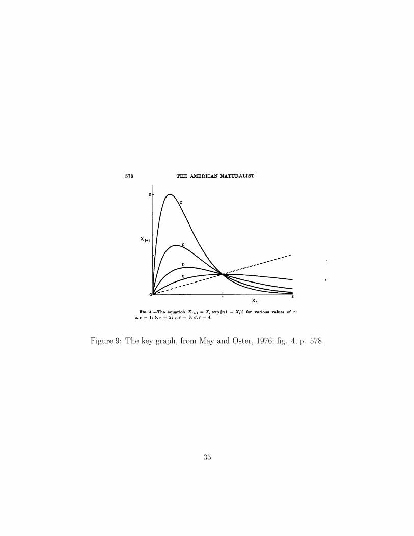
Figure 9: The key graph, from May and Oster, 1976; fig. 4, p. 578.

35

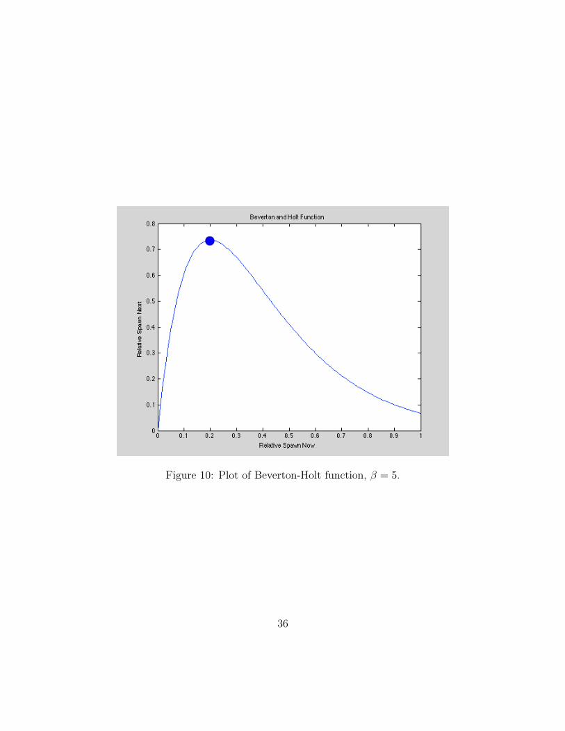
Figure 10: Plot of Beverton-Holt function, β = 5.

36

Figure 11: Beverton-Holt iteration, β = 5, α = 6.0. Compare (Beverton and Holt,1957; Fig 6.6.1, p. 57).

37

Figure 12: Beverton-Holt iteration, β = 5, α = 9.0. Compare (Beverton and Holt,1957; Fig 6.6.2, p. 57).

38

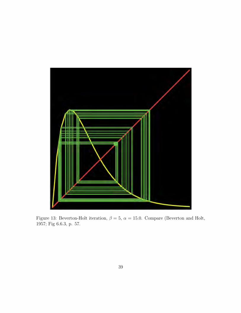
Figure 13: Beverton-Holt iteration, β = 5, α = 15.0. Compare (Beverton and Holt,1957; Fig 6.6.3, p. 57.

39

Figure 14: Beverton-Holt iteration, β = 8. Here, R = α (on the horizontal axis)increases from 4 to 20, while the domain, the unit interval [0.1], is shown as thevertical axis. For each value of R, the corresponding attractor is shown in reddirectly above.

40

Figure 15: Recruitment variability of North Sea cod (solid) and haddock (dashed).Annual recruitment (one-year old fish) in millions of tonnes from 1950 to 1995. From(Fogarty, 2001; Fig. 1).

41

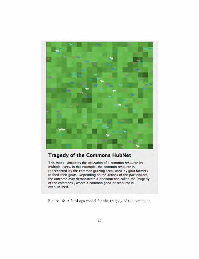
Figure 16: A NetLogo model for the tragedy of the commons.

42

Figure 17: A scheme for an all-encompassing model.

43

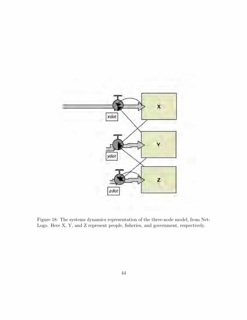
Figure 18: The systems dynamics representation of the three-node model, from Net-Logo. Here X, Y, and Z represent people, fisheries, and government, respectively.

44