Ch02 2 - Western Michigan University
49
© 2010 The McGraw-Hill Companies Communication Systems, 5e Chapter 2: Signals and Spectra A. Bruce Carlson Paul B. Crilly
Transcript of Ch02 2 - Western Michigan University
© 2010 The McGraw-Hill Companies
Communication Systems, 5e
Chapter 2: Signals and Spectra
A. Bruce Carlson
Paul B. Crilly

© 2010 The McGraw-Hill Companies
Chapter 2: Signals and Spectra
• Line spectra and fourier series
• Fourier transforms
• Time and frequency relations
• Convolution
• Impulses and transforms in the limit
• Discrete Fourier Transform (new in 5th ed.)

3
Fourier Transform
• Time to frequency domain
• Frequency to time domain
• Condition …
dttf2jexptvfV
dftf2jexpfVtv
dttvE02
Table T.1 on pages 780-780

Table T.1: Fourier Transform Pairs
RC Filter
5
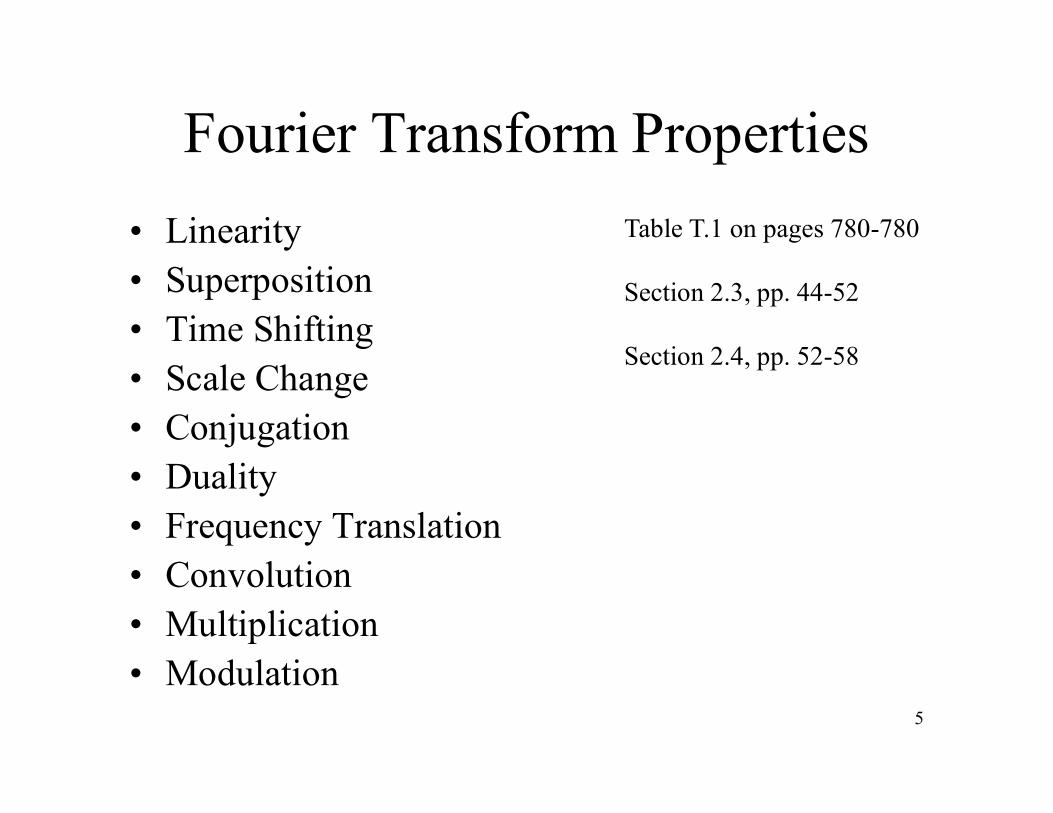
Fourier Transform Properties
• Linearity• Superposition• Time Shifting• Scale Change• Conjugation• Duality• Frequency Translation• Convolution• Multiplication• Modulation
Table T.1 on pages 780-780
Section 2.3, pp. 44-52
Section 2.4, pp. 52-58

Fourier Transform Properties
6

Note on Fourier Transforms
• Find a table
• Learn to use the table
• Yes, calculators can do it too …but after a while you should “Know” the easy or continually repeated transformations– RectSync
– Sin/Cosdelta functions at +/- f
– Exp(i*2*pi*f*t)single delta function at f
– Time delaylinear phase
– Convolution Multiplication
7

Why Know Properties• Properties may allow mathematical short cuts!
– Pre-derived simplification.
• When properties exist, the solution must obey the properties– Only incorrect solutions do not have the properties (e.g.
purely real or imaginary, symmetry, etc.)
– Check your result to see if it makes sense!
8

Two Most Important Properties
• Convolution
• Mixing
9
fWfVtwtv
fWfVtwtv *

Convolution
• Convolution in the time domain
• The Fourier Transform Pair is:
10
dtvwdtwvtwtv
fWfVtwtv
fWfVdevfW
dvefWdvdtetw
dtedtwvtwtvF
fj
fjtfj
tfj
2
22
2

Mixing
• Convolution in the frequency domain
• The Fourier Transform Pair is:
11
dfVWdfWVfWfV
fWfVtwtv *
twtvdeVtw
dvetwdVdfefW
dfedfWVfWfVF
fj
fjtfj
tfj
2
22
21
Continuing
• Continuation from previous Chapter 2-1 notes …
12
13
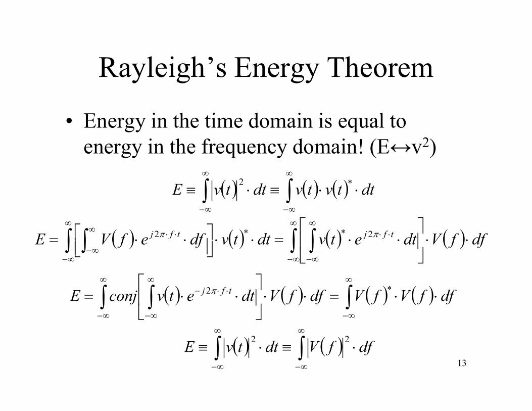
Rayleigh’s Energy Theorem
• Energy in the time domain is equal to energy in the frequency domain! (E↔v2)
dttvtvdttvE *2
dffVdtetvdttvdfefVE tfjtfj 2**2
dffVfVdffVdtetvconjE tfj *2
dffVdttvE22
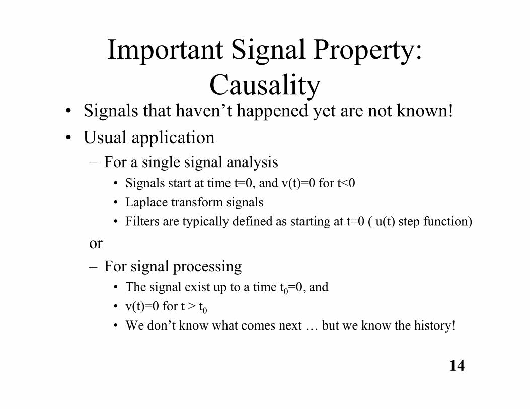
Important Signal Property: Causality
• Signals that haven’t happened yet are not known!
• Usual application– For a single signal analysis
• Signals start at time t=0, and v(t)=0 for t<0
• Laplace transform signals
• Filters are typically defined as starting at t=0 ( u(t) step function)
or
– For signal processing• The signal exist up to a time t0=0, and
• v(t)=0 for t > t0
• We don’t know what comes next … but we know the history!
14

Causality and Filtering• Convolution Form
– The filter, h, can be defined for positive time only
– The signal, x, is defined for all past time up to time t
• Then, when limited by the filter impulse response:
15
dtxhtz
T
0
dtxhtz

16
The RC Filter: 1st order Butterworth Low Pass Filter
• Using Rayleigh’s Energy
y(t) v(t)
RC1sRC
1
sC1R
sC1
sHsY
sV
0t,RCtexp
RC
1th
dttvdffVE22

17
Homework 2.2-8
• Percent of total Energy based on the bandwidth of an “exponential” time signal impulse response at – fBW= b/2π and fBW = 4b/2π = 2b/π
0t,0
0t,tbexpAtv
b
A
b
tbAdttbAEE tv
22
2expexp
2
0
2
0
2
fjb
AfV
2
• Total Energy is:
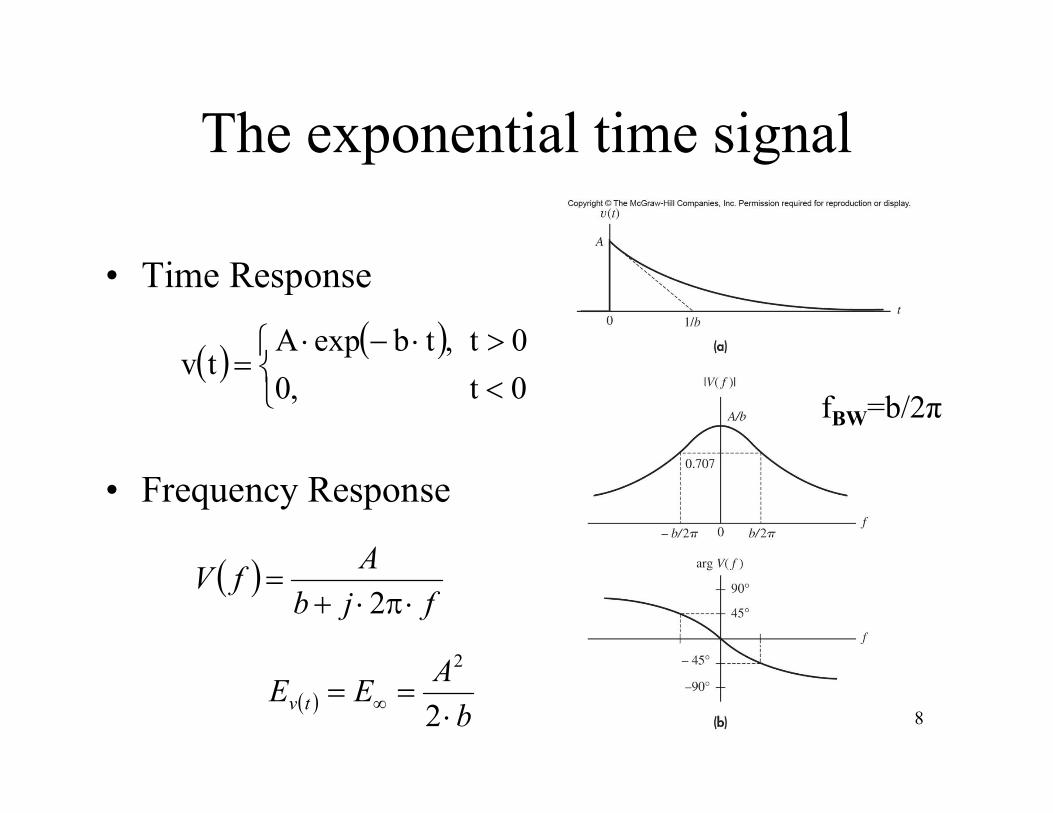
The exponential time signal
• Time Response
• Frequency Response
18
0t,0
0t,tbexpAtv
fjb
AfV
2
b
AEE tv
2
2
fBW=b/2π

19
Homework 2.2-8 (cont)• Percent of total Energy at various “Bandwidths” fBW
– fBW= b/2π and fBW = 4b/2π = 2b/π
𝑩𝑾
𝒇𝑩𝑾
𝑩𝑾
𝒇𝑩𝑾𝑩𝑾
𝐸 =𝐴
𝑗 ⋅ 2𝜋 ⋅ 𝑓 + 𝑏⋅
𝐴
−𝑗 ⋅ 2𝜋 ⋅ 𝑓 + 𝑏⋅ 𝑑𝑓
𝒇𝑩𝑾
𝒇𝑩𝑾
= 2 ⋅𝐴
2𝜋 ⋅ 𝑓 + 𝑏⋅ 𝑑𝑓
𝒇𝑩𝑾

20
Homework 2.2-8 (cont)
• Percent of total Energy at– fBW= b/2π and fBW = 4b/2π = 2b/π
• For a simple RC filter – wco is the 50% power point (w in radians/sec)
𝒇𝑩𝑾%𝑏2𝜋 =
2
𝜋⋅ tan 1 =
2
𝜋⋅𝜋
4=1
2
𝒇𝑩𝑾%4 ⋅ 𝑏
2𝜋 =2
𝜋⋅ tan 4 =
2
𝜋⋅ 𝜋 ⋅ 0.422 = 0.844
RCwb co1
𝒇𝑩𝑾%10 ⋅ 𝑏
2𝜋 =2
𝜋⋅ tan 10 =
2
𝜋⋅ 𝜋 ⋅ 0.468 = 0.937
RCA 1

21
Realizable Filters, RC Network
Notes and figures are based on or taken from materials in the course textbook: Bernard Sklar, Digital Communications, Fundamentals and Applications,
Prentice Hall PTR, Second Edition, 2001.

The Use of Percent Total Energy
• If you want to receive a finite time signal (finite energy) signal, what bandwidth “perfect” filter should you use?– For a decaying exponential signal
• 50% of the energy received at ffilter=fco1/2πRC
• 84.4% received at ffilter=4 x fco 4/2πRC
• 93.7% received at ffilter=10 x fco 10/2πRC
• We usually want 90%-99% of a “pulses” energy
• This also has implication for digital sampling rates!
22
End Lecture

Another Example
• What bandwidth “ideal” filter should be use if we want to filter a bipolar square wave and receive 90% of the power?
• Use the approach just shown …– Percent energy in frequency for one period of the
periodic square wave
– The general result is the integral of the sinc^2 function from f=0 to f=?
23

24
Modulation (Mixing)
• Frequency translation due to real or complex mixing products (multiply in time domain)
jtfjjtfjtx
tftxtz
00
0
2exp2
12exp
2
1
2cos
0
j
0
j
ff2
eff
2
efXfZ
• Using trig functions, try cosine x cosine mixingTable T.3 on pages 851-853
Convolution in freq. domain

25
Modulation (Mixing)
• Frequency translation due to real or complex mixing products (multiply in time domain)
jtfjjtfjtx
tftxtz
00
0
2exp2
12exp
2
1
2cos
0
j
0
j
ff2
eff
2
efXfZ
• Using trig functions, try cosine x cosine mixingTable T.3 on pages 851-853
Convolution in freq. domain

Table T.3
27
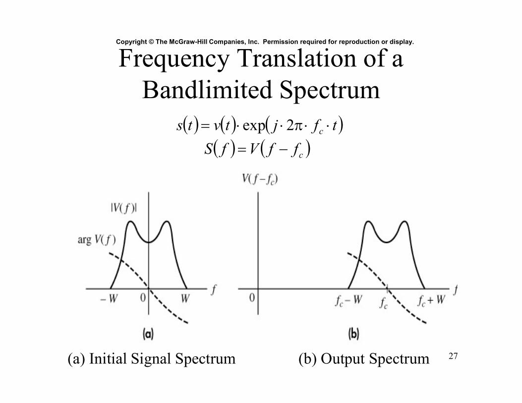
Copyright © The McGraw-Hill Companies, Inc. Permission required for reproduction or display.
Frequency Translation of a Bandlimited Spectrum
tfjtvts c 2exp
cffVfS
(a) Initial Signal Spectrum (b) Output Spectrum

Multiplication-Convolution
• Convolution in the time domain
• The Fourier Transform Pairs are:
28
dtvwdtwvtwtv
fWfVtwtv
fWfVtwtv *

29
Copyright © The McGraw-Hill Companies, Inc. Permission required for reproduction or display.
Frequency Translation: Complex Mixing tfjtvts c 2exp
cffjVfS *
(a) Initial Signal Spectrum (b) Output Spectrum

30
Copyright © The McGraw-Hill Companies, Inc. Permission required for reproduction or display.
(b) Magnitude spectrum
RF Pulse Mixing tf
tAts c
2cos
cc ffA
ffA
fS sinc2
sinc2
Is convolution easier?
(a) RF Pulse

Another Interpretation
• A limited time duration cosine waveform– window sample of an infinite periodic signal
– As the window becomes longer, the sinc gets narrower … going to an impulse as τ∞
• This is critically important when we talk about finite time sample lengths of signals.
31
tft
Ats c
2cos
cc ffA
ffA
fS sinc2
sinc2
32
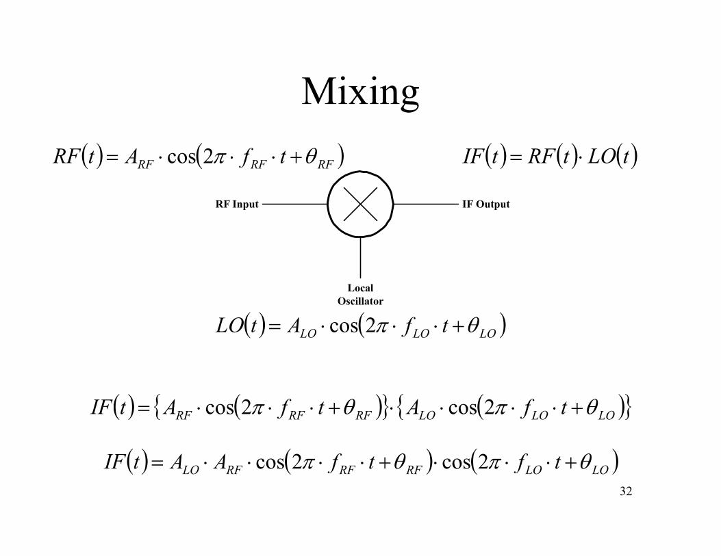
Mixing
RF Input IF Output
LocalOscillator
tLOtRFtIF
LOLOLO tfAtLO 2cos
RFRFRF tfAtRF 2cos
LOLOLORFRFRF tfAtfAtIF 2cos2cos
LOLORFRFRFLO tftfAAtIF 2cos2cos

33
Trigonometry Identities
sincoscossinsin
sincoscossinsin
sinsincoscoscos
sinsincoscoscos
cos2
1cos
2
1sinsin
sin2
1sin
2
1cossin
cos2
1cos
2
1coscos
sin2
1sin
2
1sincos
Table T.3 on pages 851-853

34
Mixing (2)
• Restating
• Using an Identity
• Ideal Low Pass Filtering

35
Spectral Equivalent – Real Mixing
• The mixing of a real RF input with a real Cosine local oscillator– Real Signal and Cosine LO spectrum
– Post mixer sum and difference spectrum
– Post Low Pass Filter (LPF) result
Real Signal
Cosine
Mixing Products
LPF
Real Signal Spectrum
Mixing Cos Signal Spectrum
Convolved Signal Spectrum
Low Pass Spectrum

36
Spectral Equivalent – Complex Mixing
• The mixing of a real RF input with a Complex local oscillator– Real Signal and Complex LO spectrum
– Post mixer sum spectrum (convolution in freq.)
– Post Low Pass Filter (LPF) result
Real Signal
Complex Oscillator
Mixing Products
LPF
Real Signal Spectrum
Mixing Exp Signal Spectrum
Convolved Signal Spectrum
Low Pass Spectrum

37
Higher Order Mixing
Mixers in Microwave Systems (Part 1)Author: Bert C. Henderson WJ Tech-note
http://www.rfcafe.com/references/articles/wj-tech-notes/Mixers_in_systems_part1.pdf
Part of WJ Comm. Technical Publicationshttps://www.rfcafe.com/references/articles/wj-tech-notes/watkins_johnson_tech-notes.htm
Watkins-Johnson (1957-2000) and later WJ Communications (2000-2008) was acquired by Triquint (1985-2014) which merged with RF Micro Devices and is
now called Qorvo (RF Solutions for 5G and beyond)https://www.qorvo.com/
https://www.qorvo.com/products
38
Convolution
• Filtering of unwanted spectral components is performed by filtering. – Convolution in the time domain
– Multiplication in the frequency domain
39
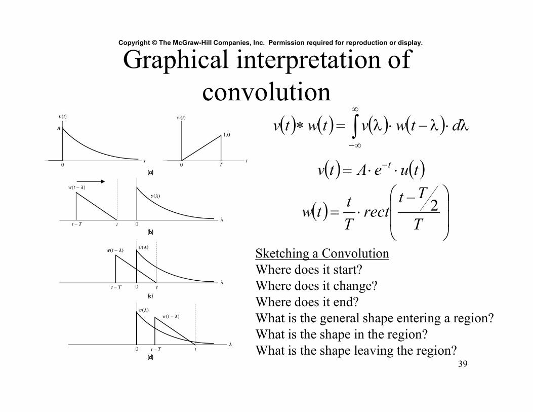
Copyright © The McGraw-Hill Companies, Inc. Permission required for reproduction or display.
Graphical interpretation of convolution
dtwvtwtv
Sketching a ConvolutionWhere does it start?Where does it change?Where does it end?What is the general shape entering a region?What is the shape in the region?What is the shape leaving the region?
tueAtv t
T
Ttrect
T
ttw 2

40
Copyright © The McGraw-Hill Companies, Inc. Permission required for reproduction or display.
Result of the convolution
Sketching a ConvolutionWhere does it start? 0Where does it change? T, triangle overlaps exponentialWhere does it end? neverWhat is the general shape entering a region? More than linear increaseWhat is the shape in the region? Exponential decreaseWhat is the shape leaving the region? Always inside, doesn’t happen
Now derive 2 equations: entering and decreasingAnd one value: the maximum at T

41
Impulses and Transformsin the Limit
• When dealing with discrete, inherently discontinuous message data we require appropriate mathematical methods to derive and describe the modulated waveforms.
• Signal descriptions for impulses (in time and frequency), step functions, etc. are required.– Define a continuous time, parameterized function that
approaches an impulse/step function as one of the parameters approaches infinity or zero.
– What are some of these functions.

42
Delta Function Approximations
• Rect
• Sinc
• Gaussian
t
rectt1
t
t sinc1
2
2
exp1
tt
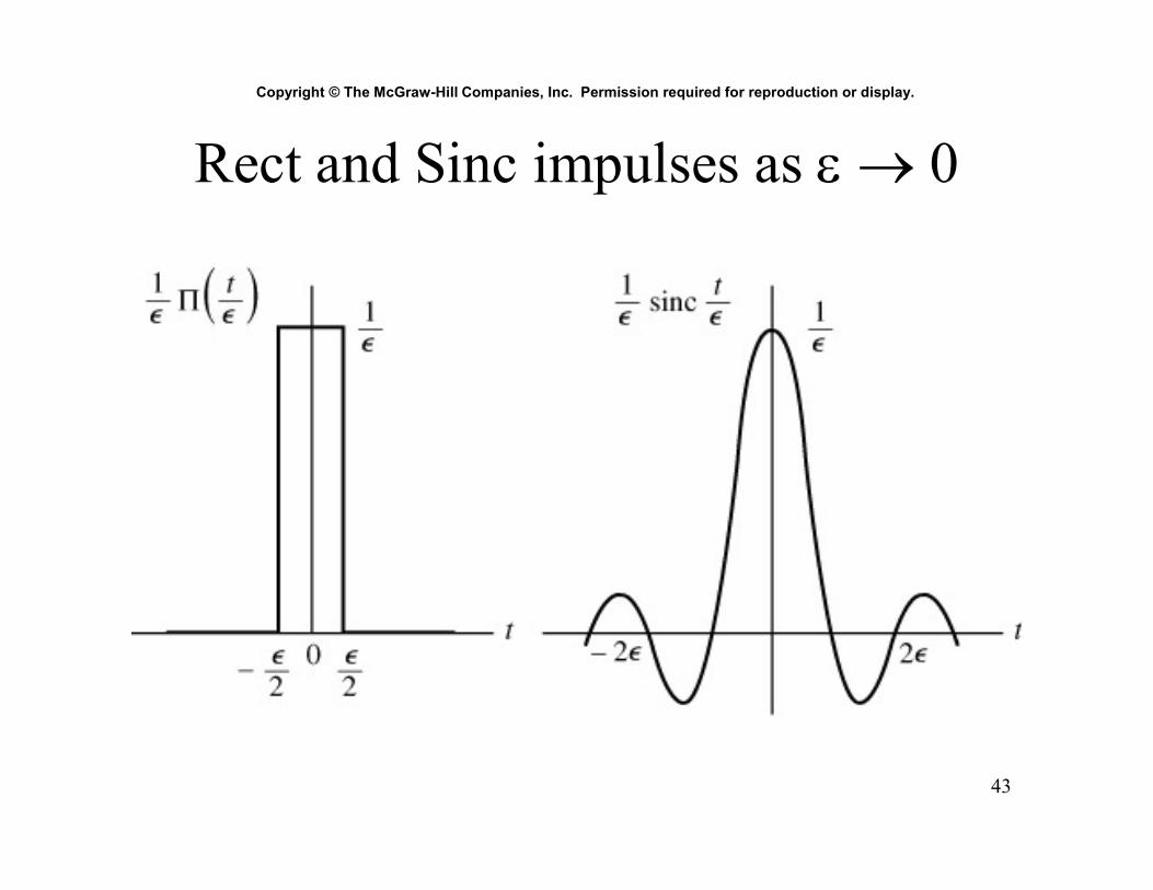
43
Copyright © The McGraw-Hill Companies, Inc. Permission required for reproduction or display.
Rect and Sinc impulses as 0

44
Impulse Properties
• Continuous sampling is equivalent to discrete samples
• Scaling
ddd tttvtttv
dd tvdttttv
𝛿 𝑎 ⋅ 𝑡 =1
𝑎⋅ 𝛿 𝑡

45
Impulses in Frequency Domain
• Transform pairs
ℑ 𝑣 𝑡 = 𝐴 ⋅ 𝛿 𝑓 = lim→
𝐴
2 ⋅ 𝑊⋅ ∏
𝑓
2 ⋅ 𝑊
𝟏
→
𝐴 ⋅ sinc 2 ⋅ 𝑊 ⋅ 𝑡 ↔𝐴
2 ⋅ 𝑊⋅ ∏
𝑓
2 ⋅ 𝑊
fAAF
AtAF

46
Signal Smoothing
• Signal approximations that provide rounding or smoothing of rapid transitions in time …– Effects of low pass filtering or attenuation of
higher frequency components.
• Inherent in transmitted signals due to component and channel effects …

47
Smoothing the Edges
• A more practical frequency domain filter:The raised Cosine filter– Cosine band edge roll-off is often used
– Easy to implement in MATLAB
• A nice explanation of finding the order of “filter roll-off” is provided in the text.

48
Copyright © The McGraw-Hill Companies, Inc. Permission required for reproduction or display.
Raised cosine pulse. (a) Waveform (b) Derivatives(c) Amplitude spectrum
Figure 2.5-7
Using Rect to Make a Filter Shape in the Time Domain
• Any continuous time signal can have a “possibly desirable” part isolated to create a filter.– Raised Cosine
– Cosine squares
– Sine single period (for odd-symmetric signals)
– Gaussian
– Main-Lobe of Sinc
• With computer tools, people can try anything!If it works, great, if not, you tried.
49