CH-02-701 Efficiency Performance and CO2 Emissions from ...

PDH-Pro.com

396 Washington Street, Suite 159, Wellesley, MA 02481 Telephone – (508) 298-4787 www.PDH-Pro.com

This document is the course text. You may review this material at your leisure before or after you purchase the course. In order to obtain credit for this course, complete the following steps: 1) Log in to My Account and purchase the course. If you don’t have an account, go to New User to create an account. 2) After the course has been purchased, review the technical material and then complete the quiz at your convenience. 3) A Certificate of Completion is available once you pass the exam (70% or greater). If a passing grade is not obtained, you may take the quiz as many times as necessary until a passing grade is obtained (up to one year from the purchase date). If you have any questions or technical difficulties, please call (508) 298-4787 or email us at [email protected].

Efficiency Performance and CO2 Emissions from Coal Power Plants

Course Number: CH-02-701 PDH: 6 Approved for: AK, AL, AR, GA, IA, IL, IN, KS, KY, LA, MD, ME, MI, MN, MO, MS, MT, NC, ND, NE, NH, NJ, NM, NV, OH, OK, OR, PA, SC, SD, TN, TX, UT, VA, VT, WI, WV, and WY

New Jersey Professional Competency Approval #24GP00025600 North Carolina Approved Sponsor #S-0695 Maryland Approved Provider of Continuing Professional Competency Indiana Continuing Education Provider #CE21800088

Power Generationfrom CoalMeasuring and Reporting

Efficiency Performanceand CO

2 Emissions

Coal is the biggest single source of energy for electricity production and its

share is growing. The efficiency of converting coal into electricity matters:

more efficient power plants use less fuel and emit less climate-damaging

carbon dioxide. This book explores how efficiency is measured and reported

at coal-fired power plants. With many different methods used to express

efficiency performance, it is often difficult to compare plants, even before

accounting for any fixed constraints such as coal quality and cooling-water

temperature. Practical guidelines are presented that allow the efficiency and

emissions of any plant to be reported on a common basis and compared

against best practice. A global database of plant performance is proposed

that would allow under-performing plants to be identified for improvement.

Armed with this information, policy makers would be in a better position to

monitor and, if necessary, regulate how coal is used for power generation.

The tools and techniques described will be of value to anyone with an

interest in the more sustainable use of coal.

TABLe oF CoNTeNTS

Foreword . . . . . . . . . . . . . . . . . . . . . . . . . . . . . . . . . . . . . . . . . . . . . . . . . . . . . . . . . . . . . . . . . . . . . . . 5

ACKNowLedGeMeNTS . . . . . . . . . . . . . . . . . . . . . . . . . . . . . . . . . . . . . . . . . . . . . . . . . . . . . . . . . . . . 7

eXeCUTIVe SUMMArY . . . . . . . . . . . . . . . . . . . . . . . . . . . . . . . . . . . . . . . . . . . . . . . . . . . . . . . . . . . . . 13

1. INTrodUCTIoN . . . . . . . . . . . . . . . . . . . . . . . . . . . . . . . . . . . . . . . . . . . . . . . . . . . . . . . . . . . . . . . 15

l 1.1 Background . . . . . . . . . . . . . . . . . . . . . . . . . . . . . . . . . . . . . . . . . . . . . . . . . . . . . . . . . . . . . . . . 15

l 1.2 objective . . . . . . . . . . . . . . . . . . . . . . . . . . . . . . . . . . . . . . . . . . . . . . . . . . . . . . . . . . . . . . . . . . . 16

l 1.3 report structure . . . . . . . . . . . . . . . . . . . . . . . . . . . . . . . . . . . . . . . . . . . . . . . . . . . . . . . . . . . . . 16

2. FACTorS INFLUeNCING Power PLANT eFFICIeNCY ANd eMISSIoNS . . . . . . . . . . 17

l 2.1 differences in reported efficiency values . . . . . . . . . . . . . . . . . . . . . . . . . . . . . . . . . . . . . 17

l 2.2 Impact of condenser-operating conditions on efficiency . . . . . . . . . . . . . . . . . . . . . . 24

l 2.3 Heat and power equivalence . . . . . . . . . . . . . . . . . . . . . . . . . . . . . . . . . . . . . . . . . . . . . . . . 26

l 2.4 efficiency performance assessment periods . . . . . . . . . . . . . . . . . . . . . . . . . . . . . . . . . . 29

l 2.5 efficiency standards and monitoring . . . . . . . . . . . . . . . . . . . . . . . . . . . . . . . . . . . . . . . . . 30

l 2.6 reporting bases for whole plant efficiency . . . . . . . . . . . . . . . . . . . . . . . . . . . . . . . . . . . 32

l 2.7 Co2 emissions reporting . . . . . . . . . . . . . . . . . . . . . . . . . . . . . . . . . . . . . . . . . . . . . . . . . . . . 33

3. GeNerIC reCoNCILIATIoN MeTHodoLoGY . . . . . . . . . . . . . . . . . . . . . . . . . . . . . . . . . . 37

l 3.1 Process boundaries . . . . . . . . . . . . . . . . . . . . . . . . . . . . . . . . . . . . . . . . . . . . . . . . . . . . . . . . . 37

l 3.2 Input data requirements . . . . . . . . . . . . . . . . . . . . . . . . . . . . . . . . . . . . . . . . . . . . . . . . . . . . . 40

l 3.3 output data . . . . . . . . . . . . . . . . . . . . . . . . . . . . . . . . . . . . . . . . . . . . . . . . . . . . . . . . . . . . . . . . 41

l 3.4 Generic corrections . . . . . . . . . . . . . . . . . . . . . . . . . . . . . . . . . . . . . . . . . . . . . . . . . . . . . . . . . 45

4. eFFICIeNCY oUTLooK For Power GeNerATIoN FroM CoAL . . . . . . . . . . . . . . . 57

9

table of contents©

OE

CD

/IE

A 2

010

10

5. CoNCLUSIoNS ANd reCoMMeNdATIoNS . . . . . . . . . . . . . . . . . . . . . . . . . . . . . . . . . . . . 61

l 5.1 IeA recommendations to the 2008 G8 Summit . . . . . . . . . . . . . . . . . . . . . . . . . . . . . . . 61

l 5.2 reporting efficiency performance . . . . . . . . . . . . . . . . . . . . . . . . . . . . . . . . . . . . . . . . . . . . 62

l 5.3 Improved collection of performance data . . . . . . . . . . . . . . . . . . . . . . . . . . . . . . . . . . . . 62

l 5.4 Performance benchmarking . . . . . . . . . . . . . . . . . . . . . . . . . . . . . . . . . . . . . . . . . . . . . . . . . 63

l 5.5 The way forward . . . . . . . . . . . . . . . . . . . . . . . . . . . . . . . . . . . . . . . . . . . . . . . . . . . . . . . . . . . . 63

reFereNCeS ANd BIBLIoGrAPHY. . . . . . . . . . . . . . . . . . . . . . . . . . . . . . . . . . . . . . . . . . . . . . . . . . 65

ACroNYMS, ABBreVIATIoNS ANd UNITS . . . . . . . . . . . . . . . . . . . . . . . . . . . . . . . . . . . . . . . . . . 69

APPeNdIX I: UNderSTANdING eFFICIeNCY IN A Power STATIoN CoNTeXT . . . . . . 75

l energy supply chain . . . . . . . . . . . . . . . . . . . . . . . . . . . . . . . . . . . . . . . . . . . . . . . . . . . . . . . . . . . . . 75

l what is efficiency? . . . . . . . . . . . . . . . . . . . . . . . . . . . . . . . . . . . . . . . . . . . . . . . . . . . . . . . . . . . . . . . 76

l The vapour power cycle . . . . . . . . . . . . . . . . . . . . . . . . . . . . . . . . . . . . . . . . . . . . . . . . . . . . . . . . . 77

l entropy and the temperature-entropy diagram . . . . . . . . . . . . . . . . . . . . . . . . . . . . . . . . . . . 79

l The Carnot cycle . . . . . . . . . . . . . . . . . . . . . . . . . . . . . . . . . . . . . . . . . . . . . . . . . . . . . . . . . . . . . . . . 80

l Supercritical steam cycles . . . . . . . . . . . . . . . . . . . . . . . . . . . . . . . . . . . . . . . . . . . . . . . . . . . . . . . . 83

l rankine and Carnot cycle efficiencies . . . . . . . . . . . . . . . . . . . . . . . . . . . . . . . . . . . . . . . . . . . . 83

APPeNdIX II: worKed eXAMPLe oF eFFICIeNCY reCoNCILIATIoN ProCeSS . . . . . 85

APPeNdIX III: reGIoNAL MeTHodoLoGIeS ANd dATA SoUrCeS . . . . . . . . . . . . . . . . . 91

l Australia . . . . . . . . . . . . . . . . . . . . . . . . . . . . . . . . . . . . . . . . . . . . . . . . . . . . . . . . . . . . . . . . . . . . . . . . 91

l Canada . . . . . . . . . . . . . . . . . . . . . . . . . . . . . . . . . . . . . . . . . . . . . . . . . . . . . . . . . . . . . . . . . . . . . . . . . 95

l China . . . . . . . . . . . . . . . . . . . . . . . . . . . . . . . . . . . . . . . . . . . . . . . . . . . . . . . . . . . . . . . . . . . . . . . . . . . 96

l Germany . . . . . . . . . . . . . . . . . . . . . . . . . . . . . . . . . . . . . . . . . . . . . . . . . . . . . . . . . . . . . . . . . . . . . . . 97

l India . . . . . . . . . . . . . . . . . . . . . . . . . . . . . . . . . . . . . . . . . . . . . . . . . . . . . . . . . . . . . . . . . . . . . . . . . . . . 98

l Italy . . . . . . . . . . . . . . . . . . . . . . . . . . . . . . . . . . . . . . . . . . . . . . . . . . . . . . . . . . . . . . . . . . . . . . . . . . . . . 100

l Japan . . . . . . . . . . . . . . . . . . . . . . . . . . . . . . . . . . . . . . . . . . . . . . . . . . . . . . . . . . . . . . . . . . . . . . . . . . . 101

l Korea . . . . . . . . . . . . . . . . . . . . . . . . . . . . . . . . . . . . . . . . . . . . . . . . . . . . . . . . . . . . . . . . . . . . . . . . . . . 102

l Poland . . . . . . . . . . . . . . . . . . . . . . . . . . . . . . . . . . . . . . . . . . . . . . . . . . . . . . . . . . . . . . . . . . . . . . . . . . 103

l russia . . . . . . . . . . . . . . . . . . . . . . . . . . . . . . . . . . . . . . . . . . . . . . . . . . . . . . . . . . . . . . . . . . . . . . . . . . . 104

l South Africa . . . . . . . . . . . . . . . . . . . . . . . . . . . . . . . . . . . . . . . . . . . . . . . . . . . . . . . . . . . . . . . . . . . . . 105

l United Kingdom . . . . . . . . . . . . . . . . . . . . . . . . . . . . . . . . . . . . . . . . . . . . . . . . . . . . . . . . . . . . . . . . . 106

l United States . . . . . . . . . . . . . . . . . . . . . . . . . . . . . . . . . . . . . . . . . . . . . . . . . . . . . . . . . . . . . . . . . . . . 109

table of contents©

OE

CD

/IE

A 2

010

11

table of contents

List of figures

Figure 2.1 Typical relationship between steam turbine heat consumption

and operating load . . . . . . . . . . . . . . . . . . . . . . . . . . . . . . . . . . . . . . . . . . . . . . . . . 19

Figure 2.2 Impact of unit operating load on heat rate . . . . . . . . . . . . . . . . . . . . . . . . . . . 20

Figure 2.3 example energy flows in a typical 500 Mw subcritical

pulverised coal-fired boiler . . . . . . . . . . . . . . . . . . . . . . . . . . . . . . . . . . . . . . . . . . 24

Figure 2.4 example of the impact of cooling-water temperature on condenser

pressure for constant unit load . . . . . . . . . . . . . . . . . . . . . . . . . . . . . . . . . . . . . . . 25

Figure 2.5 Impact of condenser pressure on heat consumption . . . . . . . . . . . . . . . . . . 25

Figure 2.6 effect of condenser fouling on turbine heat rate . . . . . . . . . . . . . . . . . . . . . . 26

Figure 2.7 effect of heat supply on overall efficiency . . . . . . . . . . . . . . . . . . . . . . . . . . . . . 28

Figure 2.8 example of relationship between Co2 emissions and net plant

efficiency (with and without CCS) . . . . . . . . . . . . . . . . . . . . . . . . . . . . . . . . . . . . 35

Figure 3.1 example of a process boundary showing energy in-flows

and out-flows for a power plant . . . . . . . . . . . . . . . . . . . . . . . . . . . . . . . . . . . . . 37

Figure 3.2 System boundary for water-steam process . . . . . . . . . . . . . . . . . . . . . . . . . . . . 38

Figure 3.3 Steam turbine plant test boundary . . . . . . . . . . . . . . . . . . . . . . . . . . . . . . . . . . . 39

Figure 3.4 Australian GeS plant boundary with co-generation . . . . . . . . . . . . . . . . . . . 39

Figure 3.5 Comparing plant performance with best practice . . . . . . . . . . . . . . . . . . . . . 43

Figure 3.6 relationship between coal GCV and as-received moisture

content for a large data set . . . . . . . . . . . . . . . . . . . . . . . . . . . . . . . . . . . . . . . . . . 46

Figure 3.7 effect of coal moisture on GCV:NCV ratio for a large data set . . . . . . . . 46

Figure 3.8 Variation of GCV:NCV ratio with GCV for a large data set . . . . . . . . . . . 47

Figure 3.9 dry, ash-free volatile matter as an indicator of carbon:

hydrogen ratio for a large data set . . . . . . . . . . . . . . . . . . . . . . . . . . . . . . . . . . 48

Figure 3.10 Approximate influence of coal moisture on plant efficiency . . . . . . . . . . . . 50

Figure 3.11 Heat rate improvement with main steam and single reheat

temperature at different main steam pressures . . . . . . . . . . . . . . . . . . . . . . . 51

Figure 3.12 Heat rate improvement at different main steam pressure, with

increasing main steam and double reheat temperatures . . . . . . . . . . . . . . 52

Figures 4.1-4.4 evolution of coal-fired heat and power plant efficiency

in selected countries . . . . . . . . . . . . . . . . . . . . . . . . . . . . . . . . . . . . . . . . . . . . . . . . . 58

Figure 4.5 efficiency improvement potential at hard coal-fired power plants . . . . . . 59

© O

EC

D/IE

A 2

010

12

table of contents

Figure I.1 Typical sequence of events in fuel utilisation . . . . . . . . . . . . . . . . . . . . . . . . . . 75

Figure I.2 Basic representation of the vapour-power cycle . . . . . . . . . . . . . . . . . . . . . . . 78

Figure I.3 Temperature-entropy diagram for steam and water . . . . . . . . . . . . . . . . . . 79

Figure I.4 Carnot cycle for steam . . . . . . . . . . . . . . . . . . . . . . . . . . . . . . . . . . . . . . . . . . . . . . 80

Figure I.5 Schematic of a simple steam cycle for power generation and associated temperature-entropy diagram . . . . . . . . . . . . . . . . . . . . . . . . 81

Figure I.6 Temperature-entropy diagram with condensed feed water heated by bled steam . . . . . . . . . . . . . . . . . . . . . . . . . . . . . . . . . . . . . . . . . 82

Figure I.7 Temperature-entropy diagram of a supercritical steam cycle . . . . . . . . . . 83

List of tables

Table 3.1 Annual plant operating data requirements . . . . . . . . . . . . . . . . . . . . . . . . . . . 40

Table 3.2 Supplementary data requirements . . . . . . . . . . . . . . . . . . . . . . . . . . . . . . . . . . . 41

Table 3.3 Template for overall power plant assessment summary . . . . . . . . . . . . . . . 42

Table 3.4 examples of uncontrollable external constraints and controllable design parameters . . . . . . . . . . . . . . . . . . . . . . . . . . . . . . . . . . . . . . 42

Table 3.5 General plant information . . . . . . . . . . . . . . . . . . . . . . . . . . . . . . . . . . . . . . . . . . . 44

Table 3.6 Typical GCV:NCV ratios for various fuels . . . . . . . . . . . . . . . . . . . . . . . . . . . . 48

Table 3.7 Typical carbon:hydrogen ratios for various fuels . . . . . . . . . . . . . . . . . . . . . 49

Table 3.8 relative carbon-intensity factors for various fuels . . . . . . . . . . . . . . . . . . . . . 49

Table 3.9 efficiency correction factors for number of reheat stages . . . . . . . . . . . . . . 52

Table 3.10 efficiency correction factors for type of cooling system employed . . . . . . 53

Table 3.11 Heat rate correction factors for different gas treatment technologies . . 53

Table I.1 Theoretical rankine efficiency of different cycle configurations . . . . . . . . 84

Table II.1 Annual “as-run” data from operator . . . . . . . . . . . . . . . . . . . . . . . . . . . . . . . . . 85

Table II.2 Information that can be derived from the “as-run” data in Table II.1. . 86

Table II.3 Supplementary data from operator that can help detailed calculation of plant performance . . . . . . . . . . . . . . . . . . . . . . . . . . . . . . . . . . . . 87

Table II.4 Basic unit data required to calculate correction factors . . . . . . . . . . . . . . . 88

Table II.5 Calculated efficiency correction factors for the “case-study” plant . . . . . 89

Table II.6 efficiency correction factors for reference plant . . . . . . . . . . . . . . . . . . . . . . . 89

Table II.7 overall power plant assessment summary . . . . . . . . . . . . . . . . . . . . . . . . . . . 90

© O

EC

D/IE

A 2

010

executive summary

13

exeCuTive SuMMAry

Coal-fired power plants, also known as power stations, provide over 42% of global electricity supply. At the same time, these plants account for over 28% of global carbon dioxide (CO2) emissions. This report responds to a request to the IEA from G8 leaders in their Plan of Action on climate change, clean energy and sustainable development, issued alongside the G8 Gleneagles Summit communiqué in July 2005. The G8 requested a review and assessment of information on the energy efficiency of coal-fired power generation. This report reviews the methods used to calculate and express coal-fired power plant efficiency and CO2 emissions, and proposes a means to reconcile differences between these methods so that comparisons can be made on a common basis. With a clearer understanding of power plant efficiency and how to benchmark this performance measure, policy makers would be in a better position to encourage improvements in power plant performance.

An essential part of sound policy development is the rigorous analysis of information which should be internally consistent and verifiable. Reliable power plant operating information is not easy to obtain, whether for an individual unit or for a number of units comprising a power plant, particularly efficiency-related information such as coal quality, coal consumption and electricity output. It is therefore proposed that an international database of operating information for units at coal-fired power plants should be established for the purposes of determining, monitoring, reporting, comparing and projecting coal-fired power plant efficiencies and specific CO2 emissions on an annual basis. Such a database of individual units could be maintained by the IEA through its Energy Statistics Division or by the IEA Clean Coal Centre Implementing Agreement as an extension of its existing CoalPower5 database of world coal-fired power plants.

At present, there is no common standard for collecting and compiling coal-fired power plant efficiency or CO2 emissions data; many different bases and assumptions are used around the world. Defining a common methodology to rationalise efficiency reporting is not a practical proposition. Instead, approximate corrections are proposed, requiring only limited information that can be collected even where the detailed bases of the original calculations are not known. Average figures, reported for periods of a month or more, will be inherently more reliable, reflecting the actual efficiency achieved more accurately than design values, performance guarantees or results from short-term tests under ideal conditions. The corrected data can then be compared with one another and to reference data sets reflecting best practices.

CO2 capture and storage, once adopted, will impact significantly on the efficiency of both existing and future plants. At the current state of technology, units retrofitted with CO2 capture would suffer a decrease in efficiency of up to 12 percentage points, and consume perhaps 20% to 30% more fuel per unit of electricity supplied. While a concept of what constitutes “capture-ready” exists for new power plants, it may not be economic or technically viable to retrofit existing plants with CO2 capture, especially at smaller inefficient units. Refurbishments will often be necessary to improve efficiency at existing plants before CO2 capture retrofit can be contemplated.

© O

EC

D/IE

A 2

010

executive summary

14

Policy makers must reflect on what steps are now needed to improve the overall efficiency of power generation from coal. This report presents the tools for analysis and makes recommendations on how to use these tools to compare performance. This will allow poorly performing plants to be identified, wherever they are located. The costs and benefits of refurbishing, upgrading or replacing these plants can be estimated as the first stage in developing new policies that would encourage greater efficiency. The prize is large; some estimates suggest that 1.7 GtCO2 could be saved annually. However, securing this reward would demand a major realignment of national energy and environmental policies, a realignment that may be less politically acceptable than allowing old, inefficient coal-fired power plants to continue running, in the hope that they will eventually fade away. Given that there currently appears to be no prospect of meeting global electricity demand without coal, governments must implement policies that respond more proactively to the growing use of coal, rather than wishing it away. Monitoring the efficiency of power plants and targeting those that perform poorly would be an important step in that direction.

© O

EC

D/IE

A 2

010

15

introduction

1. iNTroduCTioN

1.1 Background

Coal is the world’s most abundant and widely distributed fossil fuel with reserves for all types of coal estimated to be about 990 billion tonnes, enough for 150 years at current consumption (BGR, 2009).1 Coal fuels 42% of global electricity production, and is likely to remain a key component of the fuel mix for power generation to meet electricity demand, especially the growing demand in developing countries. To maximise the utility of coal use in power generation, plant efficiency is an important performance parameter. Efficiency improvements have several benefits:

• prolonging the life of coal reserves and resources by reducing consumption;

• reducing emissions of carbon dioxide (CO2) and conventional pollutants;2

• increasing the power output from a given size of unit; and

• potentially reducing operating costs.

The calculation of coal-fired power plant efficiency is not as simple as it may seem. Plant efficiency values from different plants in different regions are often calculated and expressed on different bases, and using different assumptions. There is no definitive methodology.3

In their 2005 Plan of Action on climate change, clean energy and sustainable development, agreed at the Gleneagles Summit in 2005, G8 leaders addressed this topic (G8, 2005):

“We will support efforts to make electricity generation from coal and other fossil fuels cleaner and more efficient by: (a) supporting IEA work in major coal using economies to review, assess and disseminate widely information on energy efficiency of coal fired power plants; and to recommend options to make best practice more accessible.”

Their commitment provided a sound basis for a review of how power plant efficiency data are prepared, disseminated and used, including how different methods can be reconciled. A better understanding of power plant efficiency leads quickly to the question of how it might be improved through further development and dissemination of technologies that are not yet widely deployed.

1 Quantity that is estimated to be economically recoverable using current mining techniques.

2 A one percentage point improvement in efficiency can result in a 2.5 percentage points reduction in CO2 emissions.

3 For example, the heat rate of European power plants can appear to be 8%-10% lower than their US counterparts (and so appear 3-4 percentage points more efficient). This may be partly due to real plant differences, but differences between calculation methodologies for identical plants can also be of this magnitude.

© O

EC

D/IE

A 2

010

1.2 Objective

Measuring coal-fired power plant efficiency consistently is particularly important at the global level, yet significant regional differences exist. Similarly, at the local level, the performance of individual generating units and power plants can only be compared if measured consistently. Although variations in efficiency may arise from differences in plant design and maintenance practices, the practical and operational constraints associated with different fuel sources, local ambient conditions and electricity dispatch all play significant roles. Misunderstanding these factors can result in the misinterpretation of efficiency data.

Thus, reconciling different efficiency measurement methodologies is not simply concerned with theoretical design efficiency, but with the actual operational efficiency of existing power plants and all the associated issues and constraints found in the real world.

This study proposes a generic methodology which can be applied to determine the efficiency and specific CO2 emissions of coal-fired power generation processes. The application of such a reference methodology would provide a potential route to gauge how coal might be deployed more cleanly and efficiently in the future. To this end, the major objective of this report is to review the methods used to calculate and express coal-fired power plant efficiency and CO2 emissions, and determine whether these can be reconciled for comparison using a common basis.

The target audience for this report includes technical decision makers in industry and policy makers in government who must master the details of efficiency measurement if they are to effectively manage and regulate power plants. Early conclusions from this report guided IEA policy recommendations on cleaner fossil fuels presented to the G8 Hokkaido Summit in 2008 (IEA, 2008).

1.3 Report structure

Section 2 explores, in some technical detail, those aspects of power plant design, monitoring and operation that can influence efficiency measurement and comparison. A generic methodology is prescribed in Section 3 to adjust reported data and reconcile efficiencies reported on different bases. Section 4 briefly looks at historic and likely future trends in power plant efficiency. Section 5 summarises recommendations made by the IEA at the G8 Hokkaido Summit and makes further recommendations to implement the methodology and compile a database of efficiency data that would allow the performance of power plants to be contrasted and compared. Appendices support the main report with additional technical background, an example efficiency calculation and accounts of how power plant efficiency and emissions are measured and reported in a number of different IEA member and non-member countries, all being large users of coal for power generation.

introduction

16

© O

EC

D/IE

A 2

010

2. FACTorS iNFLueNCiNG Power PLANTeFFiCieNCy ANd eMiSSioNS

This section explores aspects of power plant design and operation that influence efficiency performance. It focuses on practical issues; to aid understanding of the discussion, some theoretical aspects of power plant efficiency are set out in Appendix I. The section also reviews the relevance of current power plant performance measurement standards and how these might be reconciled using a common methodology to allow performance benchmarking. The section continues with a summary of the reporting bases and the required information sources for calculating the efficiency of a whole plant according to national standards. CO2 emissions from fossil fuel use are closely related to plant efficiency and the section concludes with a review of how these are monitored and reported in practice.

2.1 Differences in reported efficiency values

Apparent efficiency differences

Differences in reported efficiencies between plants can sometimes be artificial, and not reflective of any underlying differences in their actual efficiencies. The reported efficiency of two identical plants, or even the same plant tested twice, could potentially be different owing to:

• the use of different assessment procedures and standards;

• the use of different plant boundaries and boundary conditions;

• the implementation of different assumptions or agreed values within the scope of a test standard;

• the use of different operating conditions during tests;

• the use of correction factors to normalise test results before reporting;

• the expression of results on different bases (e.g. gross or net inputs and outputs);

• different methods and reference temperatures for determination of fuel calorific value (CV);

• the application of measurement tolerances to the reported figures;

• differences in the duration of assessments;

• differences in the timing of assessments within the normal repair and maintenance cycle;

• errors in measurement, data collection and processing; and

• random performance and measurement effects.

These effects are difficult to quantify, especially when assessing the performance of major sub-systems that are interconnected with other parts of the plant.

factors influencing Power Plant efficiency and emissions

17

© O

EC

D/IE

A 2

010

18

Gross and net values

Assessments of efficiency often refer to “gross” or “net” bases, both for the determination of the heating values of fuel inputs and for the energy outputs from a process. In the latter case, the terminology usually relates to the use of a proportion of the output energy by the process itself: the output being referred to as “gross output” before any deduction, or “net output” after the deduction for own-use. This most commonly applies to the consumption of electrical power by a plant where “generated” power is referred to as “gross output”, and “sent-out” power, following deduction of on-site power use, is referred to as “net output” or “gross-net”. This analysis can be complicated further for multi-unit sites where some parts of the process may be fed directly from a common import power supply, shared between all generating units. This power must also be deducted from generated power to derive a true “net output” for the plant; an output that may be referred to as “gross-net-net” or “station net export”.

For fuels, the difference between gross calorific value (GCV) and net calorific value (NCV) stems from the assumptions made about the availability of the energy present in the moisture in the combustion products.4 The GCV measures all the heat released from fuel combustion, with the products being cooled back to the temperature of the original sample. In the NCV assessment, it is assumed that water in the combustion products is not condensed, so latent heat is not recovered. Using the NCV basis is questionable: a modern condensing boiler could potentially achieve a heating efficiency in excess of 100%, in violation of the first law of thermodynamics. Although some regions and industries prefer to use lower heating values in daily business, the true energy content of a fuel is its GCV or higher heating value. Another complication, associated with fuel heating values, is the reference temperature used for their determination. Typically, calorific values are quoted based on a 25 °C reference temperature; however, 15 °C is also commonly used and other temperatures may be used after correction, if these differ from the temperature of the reactants and products at the start and end of the combustion test. Obviously, the use of values calculated on different reference temperature bases would result in different apparent heat inputs. Some technical standards provide equations for the correction of calorific values between different reference temperatures.

Electrical power imports and exports

Electricity produced and consumed within the plant should not affect plant performance assessment, providing the system boundary is drawn at the outer plant boundary. Electrical power imported into the plant can be deducted directly from exported power in order to calculate the overall net power generation for efficiency assessment. In general, it is recognised that power exports should be referenced to the conditions at the transmission side of the generator transformer and thus account for transformer losses.

Efficiency differences due to real constraints

It is reasonable to expect that there will be differences in efficiency between particular plants because of the constraints within which they were constructed and operate. Considerations which can impact significantly on efficiency include:

• fuel moisture content (influences latent and sensible heat losses);5

• fuel ash content (impacts on heat transfer and auxiliary plant load);

• fuel sulphur content (sets design limits on boiler flue gas discharge temperature);

• use of closed-circuit, once-through or coastal cooling-water systems (determines cooling-water temperature);

• normal ambient air temperature and humidity;

4 GCV is also known as higher heating value (HHV), while NCV is also know as lower heating value (LHV). GCV measures a fuel’s heat of combustion assuming all water in the flue gas is condensed; NCV excludes this latent heat.

5 Latent heat is absorbed or released during a change of state with no change in temperature, e.g. boiling a liquid to a gas, or condensing a gas; sensible heat is associated with changes in temperature, e.g. superheating steam.

factors influencing Power Plant efficiency and emissions©

OE

CD

/IE

A 2

010


19

• use of flue gas cleaning technologies, e.g. selective catalytic reduction (SCR), fabric filtration, flue gas desulphurisation (FGD) and CO2 capture (all increase on-site power demand); and

• use of low-NOx combustion systems (requires excess combustion air and increases unburned carbon).

A plant designed for high-moisture, high-ash coal, fitted with FGD and bag filters, and operating with a closed-circuit cooling system, for example, could not be expected to achieve the same efficiency as one without FGD using high-rank, low-ash, low-moisture bituminous coal at a coastal site with cold seawater cooling. In most cases, there is little that can be done to mitigate these effects; it is sufficient to recognise that their impact is not necessarily a result of ineffective design or operation, but merely a function of real plant design constraints.

It might be argued that the major fuel factors – the first three bullet points above – are not genuine constraints since, in many cases, fuels can be switched, blended or dried. The commercial feasibility of doing this will depend partly on the availability of fuels and partly on the cost and practicality of purchasing and transporting these to the plant. Coastal power plants may have more fuel supply alternatives than inland power plants close to local coal resources. Another obvious consideration is the environmental impact of transporting fuel over longer distances.

Efficiency differences in operation

Efficiency is significantly affected when plants operate under off-design conditions, particularly part-load operation.

Average operating load

Plants which operate with a low average output will return low efficiencies compared to their full-load design efficiency. Steam turbine heat consumption is characterised by a relationship known as the “Willans line”, shown in Figure 2.1 for an example turbine. This line shows that total heat consumption comprises a fixed element and an incremental element: at zero load, the heat consumption is not zero. This relationship is normally derived by undertaking a number of heat consumption tests on a turbine at different loads and then plotting a best-fit line through the observed values.

Figure 2.1: Typical relationship between steam turbine heat consumption and operating load

Heatco

nsu

mption

(GJ/

h)

Heat consumption = 7.289 MW + 180.0 GJ/hno-load 6.59%

Load (MW)

3 600

3 200

2 800

2 400

2 000

1 600

1 200

800

400

0

75 150 225 300 375 4500

source: gill (1984). reprinted by permission of the publisher. © elsevier, 1984.

© O

EC

D/IE

A 2

010

The overall energy consumption of a plant can be similarly characterised by a fixed element and a variable element proportional to output. Hence, overall efficiency will decline as load is reduced and the no-load portion becomes a greater fraction of the total heat.

Another related consideration is that works power6 will account for a greater percentage of generated power at part load, because the no-load running losses of electrical equipment increase relative to useful output and because certain activities must be carried out, irrespective of unit load.

For these reasons, power plants may formally record “part-load loss” as a penalty incurred purely as a result of being asked to operate the plant at a lower-than-optimum output.

Figure 2.2, derived from the Willans line and assuming an overall unit fixed heat rate of 9% (i.e. greater than the turbine-only fixed heat rate), illustrates the effect of running at lower loads on the performance of subcritical and supercritical units. Supercritical units are shown to experience only about half the part-load efficiency degradation of a conventional subcritical unit.

Figure 2.2: impact of unit operating load on heat rate

Heatra

tein

crease

(%)

Operating load as proportion of design maximum continuous rating (% MCR)

Subcritical unitsSupercritical units

24

22

20

18

16

14

12

10

8

6

4

2

0

30 40 50 60 70 80 90 100

source: e.on uk plc.

Load factor

The effects of average operating load (see above) and load factor are different. Load or capacity factor describes the output over a period of time relative to the potential maximum; it depends on both running time and average operating load. It is not necessary to consider load factor specifically here since the impacts of more frequent unit starts or lower operating unit loads can be taken into account separately. It is technically possible for a low load factor plant to attain high efficiency if starts are few in number and the load is kept high during the periods of generation. However, there may be practical issues relating to system power demand and management which preclude operation in this way.

6 “Works power” is the electricity used on a power plant site, principally to power motors that drive pumps, fans, compressors and coal mills.


20

© O

EC

D/IE

A 2

010

Transient operation

Another factor which can significantly impact efficiency is the number of perturbations (transients) from steady state operating conditions. During each of these transients, the plant will not be operating at peak performance: the more transients, the greater the reduction in efficiency. Operation in frequency response mode, where steam flow and boiler firing fluctuate to regulate system frequency, can lead to more transients. Other situations may require frequent load changes, notably in response to power system constraints or power market pricing.

Plant starts

An extreme form of transient operation is where demand falls sufficiently to require plant shutdown. This incurs significant off-load energy losses, particularly during subsequent plant start-up, which must be done gradually to avoid damage from thermal stresses. While the plant is not generating output, all of the input energy is lost (i.e. efficiency is 0%). Supercritical units, in particular, have high start-up losses because large quantities of steam, and therefore heat energy, must be dumped to the condenser during start-up.

Power plants operating in volatile or competitive markets, or operating as marginal providers of power, may be required to shut down frequently. This can, in turn, lead to a deterioration in physical condition which will affect plant efficiency. For base-load operation, unit start-up energy may be a negligible fraction of total energy (<0.5%). For other flexibly operated plant it could represent 5% or more of total energy consumed and result in reductions in efficiency in the order of 2 percentage points, even if the average output during the on-load period is high. For simplicity, corrections of 0.5%, 1.5% and 5% of total energy use could be applied to plant running regimes categorised as “base-load”, “transitional” and “marginal/peaking”.

Performance optimisation

The adoption of good practices and exercise of care will avoid most operational problems within the control of a plant operator. Although the majority of operational efficiency variations are linked to unit load and the need to operate through transient conditions, there is usually some scope for final optimisation of performance by fine tuning of automatic controller set points and control loops, amounting to about 1% of a unit’s heat rate. Optimisation may be performed manually or through the use of advanced control systems or optimisers, some of which are based on neural networks. Operator experience can also be a source of operational gains or losses. The commercial attractiveness of performance optimisation increases with plant load and can be substantial at high loads. Optimisation is a potentially attractive proposition at any load where the plant will be operated for a significant period of time.

Boiler operation is an area where efficiency gains are often possible. A “fixed-pressure” boiler requires the outlet steam to be throttled at part load to match the lower pressure demand of the turbine. “Sliding-pressure” boiler designs avoid this loss, with the added benefit that feed-water pumps require less power. Sliding-pressure control is standard operating procedure on most modern power plants.

Control systems play a major part in optimisation by enabling the automation of best practices. The use of advanced control systems can bring about significant efficiency improvements and reduce CO2 emissions.

Regulation

The regulatory environment can have a significant impact on power plant operation and efficiency. Meeting the requirements of environmental emissions legislation, even where flexible with respect to operating regime and fuel quality, can be a challenge to operators. In some cases, achieving multiple objectives simultaneously can impact efficiency since transients, off-design fuels and emission controls generally add to energy losses. Functional performance, for example to achieve target output, load ramp rates or frequency control, may be a higher priority to the plant operator than efficiency optimisation. Where a plant operates within a competitive market environment, making the case for investment in plant maintenance and upgrades to improve performance and efficiency may be more difficult because operating margins may be slim, and market volatility may hinder long-term investment planning.


21

© O

EC

D/IE

A 2

010

Efficiency differences due to design and maintenance

For the same operating regime and boundary conditions, any remaining differences in efficiency are largely down to the basic design of the plant and how well it is maintained. Overall performance is generally a function of both individual component design efficiencies and process integration. Lower levels of performance can be expected from plants of older design, although upgrades can improve even the oldest plants.

Plant design

The adoption of supercritical (SC) and ultra-supercritical (USC) steam conditions for new generating plants, in conjunction with modern steam turbine designs, has been key to improved design efficiency.7 Newer plant designs may also incorporate steam temperature attemperation control, which results in lower steam-cycle losses, and better control and optimisation features.

Comparisons of best practice are generally confined to this area since factors such as plant operating regime, fuel quality and local ambient conditions are largely beyond the control of the plant owner and operator.

Deterioration

Taking turbine efficiency as an example, deterioration over the first year of operation could be relatively rapid, but will then slow. Deterioration may be the equivalent of 0.25% of heat consumption per year of operation between overhauls, but with up to 2% lost in the first two years alone. This reduction in turbine efficiency will be reflected in overall plant performance. Some, but not all, of the deterioration will be recovered by routine maintenance. Generally, plant performance will be restored during major overhauls. However, the extent of repair and refurbishment work, and the ensuing efficiency benefits, is a commercial decision for the operator.

Plant maintenance

The actual performance of a plant compared to its design and “as-commissioned” performance is crucial. As equipment wears, fouls, corrodes, distorts and leaks, as sensors and instrumentation fail, and as calibrations drift, the plant tends to become less efficient. As well as ensuring integrity, a key requirement of plant maintenance is to maintain peak efficiency. Improved maintenance and component replacement and upgrading can reduce energy losses.

In addition to restoring performance lost through in-service deterioration, plant maintenance and overhaul activities represent an opportunity to retrofit more modern components with improved performance. Where plant designs have improved since original plant commissioning, the combination of performance restoration and plant modernisation can lead to substantial improvements in efficiency and often to greater generating capacity.

In practice, any poorly performing auxiliary equipment or individual components (e.g. fans, pumps, heat exchangers, vent and isolation valves, gearboxes, leaking flanges and even missing or inadequate insulation) contribute to the overall deterioration of plant performance over time, compounding the effects of deterioration in major components, such as the steam turbine. Significant deterioration can also occur in the steam turbine condenser or cooling-water system, where progressive increases in air ingress and steam- and water-side fouling or corrosion can degrade heat transfer. Cooling tower performance is an important consideration in this respect.

Component availability

Efficiency can be reduced by the non-availability of certain items of plant and equipment including:

• main condenser cooling-water pumps and condenser tube banks;

7 Subcritical, supercritical and ultra-supercritical are engineering terms relating to boiler temperature and pressure conditions (see Appendix I).


22

© O

EC

D/IE

A 2

010

• cooling towers;

• on-load condenser cleaning equipment;

• condenser air extraction plant;

• boiler feed-water pump turbine and feed-water heaters;

• reserve coal milling plant capacity;

• feed-water heater drains pumps (resulting in diversion of drains to the condenser); and

• boiler soot blowers.

Maintaining cleanliness is important to avoid heat transfer degradation in boilers, condensers and cooling-tower systems. Accumulated deposits in a steam condenser will result in higher turbine backpressure; in tubular feed-water heaters, they will increase terminal temperature difference; and in the boiler, they will increase gas exit temperatures. For the boiler in particular, the lack of availability of individual soot blowers can lead to severe deposit formation which can affect the combustion process, and cause erosion and thermal-stress damage. In bad cases, such deposits can force unit de-rating or even plant shutdowns. Even in cases with no forced outage, an increase in planned outages and internal cleaning costs may still be incurred.

Abnormal operating conditions brought about by faulty instrumentation or equipment can result in significant efficiency losses which will accumulate if left uncorrected. Failed valve actuators, missing indicators and out-of-tune control loops can leave units operating with some equipment out of service, or with restricted control facilities and flexibility.

Energy and efficiency losses

The transfer of heat energy to the working fluid of the power cycle can never be complete or perfect. The presence of tube wall and refractory material (if used), surface deposits and non-ideal flow regimes all impede heat transfer. In the case of a coal-fired boiler, the net result of these imperfect conditions is a degree of heat loss from the hot source (burning coal) in the form of hot flue gases. In cases where condensation has to be avoided, and particularly where the acid dew point temperature is raised because of the presence of sulphur, chlorine or excessive moisture in the fuel, the hot flue gases loss can be significant. Auxiliary equipment consumes energy, e.g. coal mills, water pumps, fans and soot blowers for cleaning heat transfer surfaces. Some heat is also lost to the surroundings through conduction, convection and radiation of heat, even where equipment is insulated. The turbo-alternator plant similarly has losses which reduce performance compared to the ideal, and although efforts are made to minimise these, there are economic and practical limits to what can be achieved.

In summary, the plant will have losses associated with:

• combustor flue gas wet and dry gas losses and unburned gas heating value;

• combustor solid residue sensible heat content and unburned fuel heating value;

• heated water or steam venting and leaks, and other drainage and blow-down;

• frictional losses, radiated and convected heat;

• cooling system losses where heat is rejected and not recovered;

• heat lost to flue gas treatment reagents and energy consumed by fans in overcoming gas pressure drops;

• make-up and purge water;

• off-load losses associated with start-up and shutdown;

• off-design losses associated with transient operation and part-load running; and

• transformer losses.


23

© O

EC

D/IE

A 2

010


24

2.2 Impact of condenser-operating conditions on efficiency

The Sankey diagram in Figure 2.3 shows example heat flows in a typical 500 MW subcritical pulverised coal-fired boiler, where the electrical output is 39% of the heat input and the heat rejected by the condenser to the cooling water is 52.5%. This example illustrates that it is the thermodynamics of the steam cycle, and not the fuel combustion process, which is a limiting factor for conventional power plant efficiency. Where the rejected heat can be utilised, this can provide significant improvements to the overall cycle efficiency.

Figure 2.3: example energy flows in a typical 500 Mwsubcritical pulverised coal-fired boiler

Electricaloutput 39%

Feed heating 38%

Heat input 100%

Boiler losses 5.5%

Steam range and feed radiation loss 0.5%

Condenser loss 52.5%

Turbine-generator mechanical and electrical losses 1.5%

Works auxiliaries 1.0%

source: white (1991). reprinted by permission of the publisher. © elsevier, 1991.

A relatively small change in condenser pressure, in the order of thousandths of a bar (or hundreds of pascals), can bring about seemingly disproportionately large changes in plant efficiency. To achieve similar changes in efficiency at the high-temperature end of the cycle would require more significant changes in steam conditions. A major factor governing the condenser pressure is the availability of a cold heat sink for heat rejection. This is often provided in the form of a large body of water such as the sea or a river, although heat can also be rejected using closed-circuit wet, semi-dry or dry cooling systems. The temperature and quantity of cooling medium available to the condenser have a significant impact on performance. Since economics generally determine the heat exchanger size, and the capacity of the cooling system, a major factor determining real plant performance becomes the cooling-water supply temperature to the condenser. This tends to be lowest for coastal sites in the northern hemisphere and highest for sites in locations with high ambient temperatures and limited water supplies.

The precise impacts of cooling-water temperature on condenser pressure, and the associated impact of condenser pressure on heat rate, are site-specific. Like many of the other losses considered in this report, a detailed thermodynamic model in conjunction with real plant operating experience should be used to assess site specific losses. However, within reasonable limits, some approximations can be made. In general, the impact of cooling-water temperature on condenser pressure is about 2 mbar per 1 °C change in inlet temperature, and the associated impact on heat rate is in the order of 0.1% of station heat consumption per 1 mbar. Thus a difference of 5° C in cooling water inlet temperature might change unit heat consumption by around 1%.

© O

EC

D/IE

A 2

010


25

Ambient conditions change both seasonally and diurnally. In the case of a closed-circuit cooling system, there will be feedback effects from the load on other units which may be using the same cooling system. These all affect heat consumption. Examples of the impact of cooling-water temperature on condenser pressure and the impact of condenser pressure on heat consumption in conventional steam plants are shown in Figures 2.4 and 2.5.

Figure 2.4: example of the impact of cooling-water temperature on condenser pressure for constant unit load

Condenser cooling-water inlet temperature (°C)

90

80

70

60

50

40

30

20

10

0

0 5 10 15 20 25 30

Condense

rpre

ssure

(mbar)


Figure 2.5: impact of condenser pressure on heat consumption

Heatco

nsu

mption

corr

ect

ion

fact

or

Back pressure (mbar)

0.97

0.98

0.99

1.00

1.01

1.02

1.03

1.04

1.05

1.06

1.07

0 20 40 60 80 100


© O

EC

D/IE

A 2

010

Maintaining a low condenser pressure is clearly important. However, power plant condensers tend to suffer from degradation in performance over time because of scaling and fouling, as well as any loss of area due to the removal from service of damaged elements (usually by sealing). Although periodic physical cleaning is usually performed, and some stations have on-load cleaning systems, performance still varies according to the state of cleanliness. Figure 2.6 illustrates the effect of condenser cleanliness on heat consumption.

Figure 2.6: effect of condenser fouling on turbine heat rate

Rela

tive

heatra

te(%

)

Cleanliness factor (%)

60 65 70 75 80 85 90

101.8

101.6

101.4

101.2

101.0

100.8

100.6

100.4

100.2

100.0

source: ago (2006). reprinted by permission of the publisher. © department of climate change and energy efficiency, 2006.

Steam cycle efficiency can be improved by extending the working temperature range through the addition of “topping” or “bottoming” cycles. In the topping cycle, a gas turbine is employed, where the working fluid is hot gases at a higher temperature than steam in a steam turbine, and exhaust heat is used in the boiler of a Rankine steam cycle. In a bottoming cycle, refrigerant-type fluids can be used to accept the heat rejected from the Rankine cycle and do more work in a separate turbine or expander designed for the lower temperature gas. Neither option is commonly employed in coal-fired electricity generating plant, although a combined cycle gas turbine plant is effectively a topping cycle with a Rankine cycle, albeit with no direct firing of the heat recovery boiler.

2.3 Heat and power equivalence

Both heat and electrical power are forms of energy and can therefore be measured using the same engineering units. Energy conversion processes themselves can only convert heat into power with a certain efficiency; losses mean that electric power requires more primary energy than heat, making electricity more valuable. Although net power and net heat outputs can be calculated separately, the equivalence between power and heat requires careful consideration. Heat use, in particular, can be a very important factor in efficient coal energy utilisation and specific CO2 emissions.

Plants supplying both heat and power have an overall plant energy efficiency that can be calculated by taking into account both the heat and power outputs from the process. While it is also possible to calculate effective


26

© O

EC

D/IE

A 2

010

efficiencies for heat and power production independently, these values may have less meaning and require more interpretation. For example, the heat output can be used as a fuel heat rate correction to yield a net heat flow used for electricity generation.

In the case of a power production process where rejected heat is not utilised, as in most utility-scale plants, the total fuel energy input is used to produce electrical power with a given efficiency. If the waste heat was recovered and used, it could be argued that the heat was not produced specifically to meet demand, the efficiency of its production might be considered to be 100%. The use of some of this otherwise waste heat now brings about an apparent increase in plant electrical efficiency, even though nothing in the basic power production process has changed. If, however, the waste heat utilisation was excluded from the power generation efficiency, then this would not reflect the energy efficiency benefits of combined heat and power.

Some standards and protocols suggest that heat and power generation efficiencies should be calculated separately and each referred to the total energy input (usually input fuel energy, but may also include power and heat energy from other sources) as follows:

power generation efficiency =output power energy

total energy input

heat generation efficiency =output heat energytotal energy input

This provides one method of determining efficiency, although the results may be misleading. If some or all of the rejected heat from power generation is used to satisfy a heat demand, and therefore offset other energy use, this is not recognised in the power generation efficiency calculation. It is proposed that heat rejected from the steam cycle which is recovered and put to use is not considered as consumed by the power process, or treated as a loss, but is instead treated as energy supplied to the heat system.

The overall energy efficiency of the plant can then take account of power and heat export, as applicable:

plant efficiency =(output power energy + output heat energy)

total energy input

The apparent electrical efficiency can be determined by debiting any heat energy output from the total input energy. In other words, any useful energy output, other than electricity, effectively reduces the energy attributed to the generation process. For example, consider a plant with a fuel energy input of 500 GJ producing power with an energy equivalent of 200 GJ (56 MWh). The overall plant efficiency equals the power generation efficiency, because there is no heat output:

power generation efficiency =200

= 40.0%500

If 150 GJ of the waste heat is used, then the overall plant efficiency increases:

overall plant efficiency =200 + 150

= 70.0%500

The apparent electrical or power generation efficiency is now:


= 57.1%500 – 150

Similar analysis can be used to calculate the efficiency of heat production:

heat generation efficiency =150

= 50.0%500 – 200


27

© O

EC

D/IE

A 2

010

This method of analysis, although not perfect, is a practical means of calculating and comparing real plant efficiencies. In the above example, the heat generation efficiency is low compared to the efficiency of a modern heating boiler. However, the use of waste heat improves the effective efficiency of the power generation process and the overall energy efficiency. It should be noted that the overall efficiency is not the simple numerical sum of the power and heat efficiencies.

The simplicity of this calculation enables the output heat energy to be used directly as a correction factor to the overall efficiency figure of a combined heat and power plant. Figure 2.7 shows a generic correction factor which can provide corrections for a range of plant types. It should not be used to determine or correct the independent heat-only or power-only efficiencies.

Figure 2.7: effect of heat supply on overall efficiency

0.9

1.0

1.1

1.2

1.3

1.4

1.5

1.6

1.7

1.8

1.9

2.0

2.1

2.2

0 10 20 30 40 50 60

Effic

iency

multip

lier

note: efficiency multiplier = 1 / (1 - xh) where xh is the heat recovered from rejected or waste heat as a proportion of the total energy output (heat and power).

A more complex relationship and a set of power loss coefficients are described in the German VDI 3986 standard (VDI, 2000). However, this degree of complexity is rarely necessary. The VDI also calls for the heat energy to be expressed in terms of the electrical power which it would have generated had it been used in the main power process. The ASME PTC 46-1996 performance test code, from the United States, permits corrections for exported heat, although these corrections are based on modelling analysis for particular scenarios (ASME, 1997).

In a refinement to the analysis described above, European Union law requires that the heat supply be grossed up to the input energy that would have been needed to supply the same heat from a stand-alone heating boiler operating at 88% efficiency (or 86% in the case of lignite-fired plants).8 The power generation efficiency in the above example then becomes:


= 60.7%500 – 150 / 0.88

8 Directive 2004/8/EC of the European Parliament and of the Council of 11 February 2004 on the promotion of cogeneration based on a useful heat demand in the internal energy market and amending Directive 92/42/EEC was published in the Official Journal of the European Union, OJ L 52 on 21 February 2004 (pp. 50-60). Harmonised efficiency reference values for the separate production of electricity and heat were tabulated in Commission Decision 2007/74/EC (OJ L 32, 6 February 2007, pp. 183-188), with further detailed guidance in Commission Decision 2008/952/EC (OJ L 338, 17 December 2008, pp. 55-61).


28

© O

EC

D/IE

A 2

010


29

2.4 Efficiency performance assessment periods

Most generation assets, whether operated for power, heat or both, have varying capacity, load or utilisation factors. Their outputs may change depending on the time of day, season, state of the energy market or demand profiles. These changes affect performance since plants must operate under off-design conditions (e.g. transients or part-load) or face energy penalties associated with, for example, unit start-ups and shutdowns. Attempting to represent a given plant with a single performance figure is therefore almost meaningless when taken out of temporal context, even before the detail of the calculation is considered. Unfortunately, this is not often recognised in comparisons of technologies, and misleading conclusions can easily be drawn.

Potential bases upon which performance could reasonably be stated include:

• theoretical maximum (based on boundary conditions);

• as-designed (intended full load);

• as-commissioned (formal acceptance test at actual load);

• best-achieved (formal performance assessment test at actual load);

• latest or best-recent (formal performance assessment test at actual load);

• average-daily (by performance monitoring, actual load);

• average-weekly (by performance monitoring, actual load);

• average-monthly (by performance monitoring, actual load);

• average-annual (by performance monitoring, actual load);

• average inter-overhaul (by performance monitoring, actual load); and

• average cumulative-to-date (by performance monitoring, actual load).

As can be seen, the conditions of test may or may not be at the maximum rated output; and may or may not be carried out at, or corrected to, a set of standard reference conditions, including ambient temperature and pressure, and cooling-water temperature. Although tests at the rated output demonstrate the potential performance of the plant, the actual average performance may be significantly lower for the reasons discussed above.

The assessment of overall plant performance needs to establish not just what the plant was designed to, or might achieve, but what it actually does achieve under real operating conditions. It is this measure which ultimately determines the energy use of the plant and its related CO2 emissions. Although reference to a standard set of conditions might sometimes assist in the technical comparison of plants, it would generally be preferable to use the actual conditions for comparison rather than an arbitrary set of reference conditions.

Most power plants operating within a regulated environment will be required to submit annual reports and data returns from which the main information for whole plant performance assessment should be available. The advantage of adopting an annual operating period is that, irrespective of start and end dates, it will tend to smooth out many of the potentially variable factors such as ambient conditions, seasonal variations, operating regime, short-term plant problems and fuel quality to provide more confidence in the assessment. Assessments based on short-term tests will generally be over-optimistic and exclude many factors which degrade performance during normal commercial operation.

The accuracy of annual performance figures is generally good provided that they are generated within a reasonably well controlled regime. For example, fuel deliveries should be made over calibrated weighbridges and subject to CV and analysis checks, power and heat exports and imports should be measured with calibrated metering devices, and on-site stock adjustments should be taken into account. The overall accuracy of performance calculations should then be within ±2% of the actual energy consumption (or better than ±1% if calibrated belt weighers are used) for a well-managed plant, or within ±5% for a poorly managed installation.

© O

EC

D/IE

A 2

010

The problem with annual reporting is that it does not necessarily reflect the best potential performance which is possible from the plant under favourable conditions. For this reason, it is suggested that for reference, and where available, the annual performance figure is supplemented by an additional assessment based on short-term formal test data at close to rated output conditions, which should represent the best achieved performance of the unit under the prevailing test conditions. Although such tests could be done in accordance with PTC 46-1996 (ASME, 1997), it is more likely that the boiler and turbo-alternator would be tested separately and the figures combined with suitable corrections for other losses. PTC 4-1998 for boilers specifies an expected accuracy of ±3% of heat consumption (ASME, 1998). However, this must then be combined with uncertainties in the turbo-generator and site losses, so the accuracy of short-term test data is probably no better than for the longer-term assessments.

2.5 Efficiency standards and monitoring

Fired boiler performance standards

There are a number of standards for the performance assessment of coal-fired power plant boilers including:

• BS 2885:1974 (withdrawn British standard);

• DIN 1942 (German standard);

• EN 12952-15:2003 (European standard, similar to DIN 1942).

• PTC 4-1998 (current US standard); and

• PTC 4.1-1964 (1991) (former US standard, superseded by PTC 4-1998).

There are a number of major drawbacks related to the use of these standards.

• The standards are inconsistent and therefore results based on one standard cannot be compared directly with those based on another standard without considerable care.

• They permit a wide range of system boundaries, exceptions and amendments to be made by agreement between parties to the test. This means that, even though two tests may have been undertaken in compliance with the same standard on the same plant, the results may not be comparable. Furthermore, tests on different plants are unlikely to be directly comparable. Clarification of the detailed basis on which a test result has been calculated requires more information than would be reasonable for the purposes of generating overview comparisons of plant performance.

• These test codes focus on the assessment of the boiler which, although very important, is only one component of a coal-fired power plant. While the boiler energy conversion efficiency is an important consideration, the turbo-generator and balance-of-plant equipment have a major bearing on the overall plant performance.

• It would be impractical to apply these standards during normal plant operation because they specify certain test conditions. Similarly, the efficiency obtained under test conditions will not be representative of normal operation.

The main purpose of boiler performance test codes is to provide a contractually binding means of assessing the performance of new, modified or refurbished plant on handover. As such, the standards are a means to an end and act as a convenient and widely accepted measure which can be used with minimal modification for establishing a plant performance benchmark, even if this is not representative of future plant performance. For the reasons outlined above, boiler performance standards are not suitable for the comparison of overall power plant performance.


30

© O

EC

D/IE

A 2

010


31

Whole power plant performance standards

In addition to the differences between boiler standards, there are also differences in the testing standards for steam turbine heat rate, such as ASTM and DIN standards, which could be as high as 2% (approximately 0.8 percentage points in unit efficiency). Problems also arise where plants include unusual design features that are not easily accommodated within standard test methods. This raises the question of whether the determination of whole plant efficiency is a more direct and appropriate method of providing efficiency data. The use of a whole plant method might also make the technology used within the plant largely irrelevant to the overall efficiency determination, reducing uncertainty and the potential for discrepancies.

Two whole-plant performance standards were considered in this study. The first, and one which is widely used for new gas-fired plant, is the US ASME PTC 46-1996 Performance Test Code on Overall Plant Performance.9 The second is the German VDI 3986 for the Determination of Efficiencies of Conventional Power Stations. The latter standard is somewhat less detailed than the ASME test code and, although relevant to this study, is not widely used outside Germany. However, they are both written around the requirement to provide a framework for short-term tests to verify that contract requirements have been met. Both standards contain clauses that mean their use cannot be relied upon to be consistent. The standards can still be deemed to have been applied, provided that the methods, boundary conditions and values used are agreed between the parties to the tests. This does not therefore guarantee a common basis for assessment, although the use of a standard of this type does provide some consistency.

In general, most large power plant contracts include efficiency specifications and guarantees based on the major plant components which are then combined by a method determined in the contract to produce an overall plant efficiency value. These whole plant efficiency values are not generally in accordance with any formal standard, although the efficiencies of sub-systems and components usually are.

Many new-build contracts use equations of the form shown below to calculate whole plant efficiency.

net electrical power output = Pg – Pa

Where Pg is the gross generated power and Pa is the auxiliary power consumption. The overall power station efficiency (ho) and heat rate is defined as follows:

ho = hB × hTG × hT

heat rate = 3 600 / ho (kJ/kWh)

Where hB is the boiler thermal efficiency, hTG is the turbo-generator thermal efficiency and hT is the transformer efficiency.

This form of component efficiency combination is acceptable only where it has been verified that all the power and energy flows have been taken into account. Although the combination of plant sub-component efficiencies appears simple, the overall efficiency depends on sub-component values which are generally derived from complex calculations based on extensive data obtained with test-grade instrumentation under carefully controlled conditions. As such, these forms of efficiency determinations are rarely performed and are unsuitable indicators of normal running performance of any plant.

PTC 46‑1996 – Performance test code on overall plant performance

This code is applicable to a number of plant types and fuels. However, it is not often applied in new plant contracts, either because it is not recognised or because there are commercial reasons to implement plant performance requirements and assessments by sub-component (e.g. boiler, turbine, heat recovery steam generator (HRSG), gas turbine, cooling system). PTC 46-1996 requires that the heat input to the plant is measured via fuel mass flow and heating value, or via heat flow and efficiency of the boiler, which must then be determined in accordance with PTC 4-1998. PTC 46-1996 is most commonly used in relation to gas-fired combined cycle plant.

9 In addition, ASME PTC PM-2010 Performance Monitoring Guidelines for Power Plants replaces a 1993 edition.

© O

EC

D/IE

A 2

010

VDI 3986 – Determination of efficiencies of conventional power stations

This standard, issued in 2000, is somewhat less extensive than PTC 46-1996 and although relevant to this study is not widely used outside of Germany. It offers a framework for short-term tests to verify that contract requirements have been met, and provides for a number of plant arrangements. The standard permits the expression of efficiency on different bases and allows deviation from the test methods by agreement of the parties. As with PTC 46-1996, there is some discussion included on the measurement methods and the associated uncertainties, as well as the required measurement equipment accuracies.

Other performance standards

Although PTC 46-1996 is the only commonly applied standard for whole plant performance assessment, there are other standards in place that set performance criteria for new plant. One example is the Australian Greenhouse Office Generator Efficiency Standards (GES). These set targets for the minimum acceptable level of performance for new power plants, depending on size and type, as a means of benchmarking. The GES is described in more detail in Appendix III.

It is generally assumed that fuel for mobile plant, on-site transport, utility vehicles and fuel handling vehicles is not included in power plant performance analysis since the energy and related CO2 emissions from these activities are negligible in comparison to the main power and heat generation activities of a power plant.

Performance monitoring

In the United Kingdom in the early 1970s, the Central Electricity Generating Board (CEGB) developed a common means of power plant performance monitoring, known as the Station Thermal Efficiency Performance (STEP) system. This system was devised by a national working party to calculate fuel consumption and monitor the performance of plants against “achievable” performance. By necessity, the system included many assumptions related to target performance and this created a degree of uncertainty associated with the calculation of allowable deviations from these targets. Parts of the assessment, including “cost-of-losses” calculations, were integrated into routine operations and later into computer-based monitoring systems.

Similar schemes have been developed elsewhere, and the rise of commercial efficiency monitoring systems has been observed over the last two decades. However, most commercially available software systems for efficiency or heat-rate monitoring have drawbacks; they depend on certain assumptions, and some rely on reliable and accurate instrumentation, such that they are only useful for monitoring performance trends rather than efficiency determination.

Many systems rely on estimating the turbo-alternator heat consumption, and therefore the fuel consumption, via a correction for estimated boiler efficiency, all based on averaged plant operating parameters and an extensive set of reference data for the plant in question. It would not be feasible to implement a system of this complexity for assessing the comparative performance of many different plants around the world or their relative potentials for improvement.

2.6 Reporting bases for whole plant efficiency

In most regions of the world, efficiency is expressed on the basis of the fuel’s gross calorific value (GCV) and net electrical power output.10 This appears reasonable for the purposes of comparison since it reflects the total energy input and useful electricity output. However, other bases are also used. In Europe, for example, it is common to express efficiency on a net calorific value (NCV) and net power output basis, reflecting the difficulty of recovering latent heat and coal trade on a net calorific value basis.11

10 See footnote 4.

11 Condensing boilers exist, but the selection of materials to avoid acid-gas corrosion adds to their capital cost.


32

© O

EC

D/IE

A 2

010

Where there are multiple units on a power station site, the “station” consumption for common services is generally not included in the efficiency determination of individual units; even for unit-based calculations, the plant boundaries, test standards and efficiency calculations can vary significantly. In most cases, unless otherwise stated, efficiencies are quoted for convenience on the basis of design, acceptance or expected maximum output efficiencies, and are generally not representative of those achieved in practice.

2.7 CO2 emissions reporting

This section explores the growing requirement to accurately measure and report CO2 emissions from fossil fuel use. The three-part ISO 14064 standard covers CO2 emissions reporting and verification (ISO, 2006).

EU Emissions Trading Scheme

The EU Emissions Trading Scheme (ETS) is the largest greenhouse-gas emissions trading scheme of its kind in the world.12 At present, the scheme requires the annual reporting of CO2 emissions by mass, similar to routine measurement and reporting undertaken in countries such as the United States. Specific emissions reporting per unit of production (e.g. gCO2/kWh) is not required. Emission calculations are based on fuel used and agreed oxidation factors. Reporting of figures on the basis of actual oxidation factors, rather than the assumed values, is permitted where actual values are available and can be verified.

Participating countries have a national allocation, agreed by the European Commission (EC), which is allocated or auctioned to major emitters by governments. Emitters must either comply with their allocated CO2 cap using the allowances they hold, buy additional allowances to cover their requirements, or pay a severe fine for exceeding their allocation (and buy the missing allowances). Allowances are freely traded and surplus allowances can be sold. Since trading began in 2005, market prices have varied considerably. Following an amendment to the ETS Directive, agreed on 17 December 2008, a greater share of allowances must be auctioned from 2013, with full auctioning generally required in the electricity sector.13

The scheme does not provide a direct means of comparing CO2 emission rates of different technologies, although the preparation of the statistics makes this possible in detail at source and by aggregation of sectors at national level.

Article 14 of the ETS Directive requires the European Commission to elaborate guidelines for monitoring and reporting greenhouse-gas emissions under the ETS; monitoring and reporting guidelines were adopted on 29 January 2004 with Commission Decision 2004/156/EC.14 Article 14 also requires Member States to ensure that emissions are monitored in accordance with these legally binding guidelines. Since 2004, the guidelines have been subject to a number of revisions (Commission Decisions 2007/589/EC, 2009/73/EC, 2009/339/EC and a draft amendment covering CCS).

Greenhouse gases and life-cycle assessment

This report focuses on energy efficiency and CO2 emissions at coal-fired power plants during fuel conversion into useful output energy. The purpose of clarifying whole plant efficiency and emissions reporting methodologies is to provide a relatively simple, common basis for relative performance assessment.

12 Directive 2003/87/EC of the European Parliament and of the Council of 13 October 2003 establishing a scheme for greenhouse-gas emission allowance trading within the Community and amending Council Directive 96/61/EC was published in the Official Journal of the European Union, OJ L 275 on 25 October 2003 (pp. 32-46). For a general description of the EU Emissions Trading Scheme, see http://ec.europa.eu/environment/climat/emission.htm.

13 Official Journal of the European Union, OJ L 140, 5 June 2009, pp. 63-87.

14 Official Journal of the European Union, OJ L 59, 26 February 2004, pp. 1-74.


33

© O

EC

D/IE

A 2

010

Emissions of methane, CO2 and other greenhouse gases associated with the extraction, preparation and delivery of fuel to power plants are not considered. Similarly, the greenhouse-gas emissions associated with the construction of coal-using plants are not taken into account in this operational assessment, although they might be considered as part of a more detailed life-cycle analysis, for example as part an environmental impact assessment for a new plant.

There are a number of published studies on methane production from mining and the carbon cost of transporting bulk commodities from which generic relationships could be created to estimate the GHG emissions footprint of coals sourced from different mines and transported over different distances using different modes of transport (e.g. Defra, 2008; Mills, 2005; and EPA, 2010).

CO2 reporting issues

Carbon or CO2

Most reporting systems in use around the world report on the basis of CO2 emissions and use factors to report other greenhouse-gas emissions as their CO2 equivalent (CO2e). Occasionally, CO2 emissions are quoted in terms of carbon (C), or confusingly are stated as “carbon” when they are in fact CO2. The equivalence in mass terms between carbon dioxide and carbon is simply the ratio of their molecular masses CO2:C, this being 3.6632 (IUPAC, 2005).

Input versus output basis

Input-based emission calculations and limits for the mass of CO2 emitted per unit of input energy, expressed in units such as tCO2/GJ or lb/MMBtu coal, create a poor comparison of specific emission rates. They imply that producing the same total emissions from the same quantity of fuel represents equivalent performance. In reality, although a more efficient plant consuming the same mass of fuel as a less efficient plant creates the same total quantity of CO2, it does so with the benefit of producing more useful output energy. Emission standards based on useful energy output (e.g. tCO2/GWh) are therefore important, since they recognise the benefits of higher efficiency and incentivise the development and implementation of cleaner, more efficient technologies.

Mass versus volume basis

Reporting gaseous emissions on a volume basis is not straightforward. Quantities must be expressed against a reference temperature, pressure, moisture and oxygen concentration if they are to be correctly compared or assessed against emission standards. In contrast, reporting emissions on a mass basis is absolute and avoids any requirement for volumetric corrections. CO2 emissions in mass units, rather than volume units, are therefore preferred and are widely used by most reporting systems and analysts.

Units of output

To report specific CO2 emissions in terms of a power plant’s useful output requires heat and electrical energy to be combined, as for the overall efficiency calculations described above. Common energy units are needed, e.g. gigajoules (GJ) or megawatt hours (MWh), with simple conversion factors between these.

Typically, large subcritical coal-fired utility plants today produce around 900 kgCO2/MWh. This figure becomes higher for high-moisture fuels, or for plants operated at low load factor or of inferior design. This can be compared to around 740 kgCO2/MWh for state-of-the-art modern supercritical plants, and potentially around 600 kgCO2/MWh for plants with advanced steam conditions that are currently under development.

Carbon dioxide capture and storage (CCS) offers perhaps the only way to make further reductions in CO2 emissions from conventional coal-fired plants. CCS would cut emissions to 60-70 kgCO2/MWh, assuming >90% CO2 capture from future state-of-the-art plants. Potentially, a net emission of zero is possible where the plant also fires a small proportion (approximately 10-15% by heat input) of biomass material to compensate for the residual CO2 emissions not captured in the plant.


34

© O

EC

D/IE

A 2

010

Figure 2.8: example of relationship between Co2 emissionsand net plant efficiency (with and without CCS)

0

200

400

600

800

1 000

1 200

1 400

1 600

25% 30% 35% 38% 40% 42% 45% 50% 55% 55%+CCS

Efficiency (LHV, net output basis)

Speci

fic

CO

em

issi

ons

(g/k

Wh)

2

Hard coal

Lignite

note: specific co2 emissions are calculated here using iPcc default emission factors for stationary combustion in the energy industries: 94.6 kgco2/gJ for bituminous coal used for power generation and 101.0 kgco2/gJ for lignite (iPcc, 2006). it is assumed that 98% of the fuel carbon is oxidised, the remaining 2% being retained in ash, although this varies in practice (iPcc, 1996). for the case shown with ccs, a co2 capture rate of 90% is assumed.

source: iea analysis.

Determination of emitted CO2

Commercial instrumentation is available for monitoring CO2 concentration and flue gas volume flows. Given the limitations of such instrumentation, the accuracy of directly measured CO2 release is probably no better than that derived by indirect calculation. Moreover, many plants do not measure flue gas volume flow and CO2 concentration, so indirect calculation of emitted CO2 is the only option and can be applied consistently.

Where FGD processes are employed for SO2 removal, the mass release (MFGD) of carbon from the reaction between limestone (CaCO3) and flue gas should be considered in the plant assessment, although its contribution to total emissions will be relatively small. The release mechanism is:

CaCO3(s) + SO2(g) + ½O2(g) + 2H2O(l) CaSO4.2H2O(s) + CO2(g)

The treatment of CO2 emissions from plant incorporating carbon capture is more difficult since the removal efficiency of the capture plant needs to be included in the calculation. It is likely that a removal efficiency factor (XCCS) of 90% or more would be achieved. The calculation of CO2 emissions must account for all these additions and reductions, such that the mass release (Mout) is:

Mout = 3.6632 × (Min + MFGD – Mash) × (1 – XCCS)

Where Min is the mass of carbon in the fuel input and Mash is the mass of unburned carbon retained in ash.

The use of further correction factors for CO2 emissions follows similar principles to those for efficiency calculations. For the purposes of developing a common plant assessment methodology, specific greenhouse- gas emissions analysis is limited only to the CO2 produced during fuel conversion into useful supplies of energy, including electricity and heat. As with efficiency, proper account must be taken of any heat supplied when calculating specific CO2 emissions per unit of electricity supplied.


35

© O

EC

D/IE

A 2

010

© O

EC

D/IE

A 2

010

3. GeNeriC reCoNCiLiATioN MeTHodoLoGy

By taking into account the factors presented in Section 2, it is possible to derive a common methodology for expressing and comparing whole plant efficiency and specific CO2 emissions relative to useful energy output for a wide range of different conversion plant types and fuels. For convenience and consistency, it is recommended that units of measurement are in accordance with the ISO 80000-1:2009 standard system (ISO, 2009). An example calculation, illustrating the methodology’s application, is included at Appendix II.

3.1 Process boundaries

To avoid the need for performance details of individual plant components, a system boundary should cover the entire power plant, from fuel reception to the interface with the power or heat transmission system. This may or may not coincide with a clear physical boundary, depending on the plant layout and its application.

Figure 3.1: example of a process boundary showing energy in-flowsand out-flows for a power plant

Power plant

Air

Fuel(s)

Make-up water

Return water

Return steam

Electric power imports

Reagents and additives

Energy in

Electric power

Hot water

Hot steam

Flue gas

Combustion residues

Fuel gas

Gas treatment residues

Energy out

Blowdown, leakage and drainage

Convection and radiation losses


generic reconciliation metHodology

37

© O

EC

D/IE

A 2

010

This approach simplifies the assessment of overall plant performance and can be applied consistently to many plant types and fuels. It also removes any debate regarding how internal energy flows, such as works power or own-use consumption, or water and steam interconnections, should be accounted for.

Such a “black-box” approach to the whole power plant island is shown in Figure 3.1, in which the energy output associated with the shaded flows can be ignored in the calculation of overall plant efficiency. Although in the short term, the measurement of some of these parameters may be subject to measurement error, the accuracy of data over longer time periods, and particularly annual periods, should be high.

A similar approach is taken in both VDI 3986 and PTC 46-1996, as shown in Figures 3.2 and 3.3.

Figure 3.2: System boundary for water-steam process

M

M

Auxiliary power

Hu

Pe,ne

mBo

G

M M

M

M

source: vdi (2000). reprinted by permission of the publisher. © vdi, 2000.


38

© O

EC

D/IE

A 2

010

Figure 3.3: Steam turbine plant test boundary

S

S

Stack

Fuel

Ash

Blowdown

Process

Test boundary

Make-up

Processreturn

Blowdown

Condensatecleaningsystem

Cooling water

Netpower

Aux. power

Steam turbine

Steamgenerator

source: asme (1997). reprinted from asme Ptc 46-1996, by permission of the american society of mechanical engineers. all rights reserved.

Similarly, Figure 3.4 is taken from the Australian GES and again illustrates the approach of using a whole-plant boundary, even where the plant cogenerates heat and power.

Figure 3.4: Australian GeS plant boundary with co-generation

Cogeneration plant boundary

Fuel

Make-up water

Electricity to grid

Powercogeneration

Imported electricityProcess

Processsteam

Condensatereturn

Power plant

Powergenerated

Aux. powerPower

sent-out

source: ago (2006). reprinted by permission of the publisher. © department of climate change and energy efficiency, 2006.


39

© O

EC

D/IE

A 2

010

3.2 Input data requirements

In order to perform an assessment of power plant performance, plant operators must ensure that they:

• weigh, or obtain weights for, all delivered fuel using calibrated equipment;

• undertake representative sampling and analysis of all fuel supplies to determine the average values of calorific value, moisture content, ash and sulphur;

• meter power import and export using calibrated equipment in order to determine net power export; and

• where applicable, meter and determine the heat content of incoming and outgoing water and steam in order to determine net heat export.

The average annual values of these parameters may then be used to determine plant performance indicators. Where there is more than one unit, such information must be provided on an overall station basis as a minimum, but the provision of supplementary information for individual units could also be required. The minimum annual data requirements for each site are shown in Table 3.1. Some basic data for each plant, discussed in more detail in Section 3.3, would also ideally be provided.

Table 3.1: Annual plant operating data requirements (to be completed by operator)

Data item Quantity Unit

Total fuel heat used (gross) PJ

Total fuel mass consumed t

Net electrical power export TWh

Net water and steam energy export (where applicable) PJ

Since light-up and stabilisation fuel is used at all coal-fired plants, they may all be considered as multi-fuel installations. This is also the case where opportunity fuels are used, such as residues and by-products from other processes or biomass energy crops. This creates some difficulty, but it should be possible to express the overall mix of fuels consumed on a bulk average mass and average CV basis.

In practice, it would be beneficial to include more detailed data to enable normalisation and better understanding, as shown in Table 3.2. It is also considered important that a brief commentary be provided to enable the context of the data to be better understood. This might, for example, provide clarification on poor reported efficiencies or note planned improvements.


40

© O

EC

D/IE

A 2

010

Table 3.2: Supplementary data requirements (to be completed by operator)


Average running load as % of maximum continuous rating (MCR) %

Average cooling-water inlet temperature °C

Average ambient temperature °C

SO2 removal efficiency %

Plant mode of operation

Fuel 1 Type

Contribution to total gross heat %

Higher heating value GJ/t

Average fuel moisture %ar

Average fuel ash content %ar

Average fuel volatiles content %ar

Average fuel sulphur content %ar

Fuel n Type

Contribution to total gross heat %

Higher heating value GJ/t

Average fuel moisture %ar

Average fuel ash content %ar

Average fuel volatiles content %ar

Average fuel sulphur content %ar

Supporting comments:

3.3 Output data

The assessment of the annual performance of a given power plant should be held in a database to facilitate

comparison with other data. The final evaluation of plant performance in accordance with the methods

described here needs to be captured in a clear and concise format, and must concentrate on the key indicators

which are relevant to the creation of the database. Part of the record for each plant needs therefore to comprise

the summary output data and part needs to comprise summary descriptive data. The summary data derived

from the proposed calculations might include those shown in the first two columns of Table 3.3. These

could be normalised and compared with best practice performance under reference conditions through a set

of corrections, as shown in Table 3.3, to judge the potential for improvement.


41

© O

EC

D/IE

A 2

010

Table 3.3: Template for overall power plant assessment summary

As-runNormalised

as-runBest practice

Normalised

best practice

Relative

performance, %

Carbon dioxide emissions

tCO2/GJ total energy output

tCO2/MWh net electrical output

tCO2/GJ net heat output

MtCO2/year

Overall plant efficiency

% GCV basis

% NCV basis

Power generation efficiency

% GCV basis

% NCV basis

Whether comparisons should be made on an “as-run” basis or a “normalised” basis is debatable. Ideally, they should be based on “as-run” figures. However, where constraints on the adoption of best practice exist, it might be more reasonable to make comparisons on a normalised basis. Normalisation of “as-run” values for comparison with “normalised best practice” values should only take into account those external factors considered to be uncontrollable constraints, but exclude controllable design parameters, as illustrated by the examples in Table 3.4.

Table 3.4: examples of uncontrollable external constraintsand controllable design parameters

Uncontrollable constraints Controllable constraints

Type of cooling-water system employed Steam conditions

Ambient temperature Plant age

Mode of plant use Unit size

Average running load Boiler feed-water temperature

Reheat pressure drop

Spray cooling requirement

Auxiliary power consumption

The “best-practice” level of performance used in the comparisons should be based on a reference data set for a specified plant of the appropriate technology type, firing a mid-range fuel composition. This best-practice reference performance can then be corrected for the actual fuel being used in order to obtain a “normalised best practice”. The normalised best-practice correction should be based on composite fuel types and properties, covering lignite, sub-bituminous coal, bituminous coal and anthracite, sometimes co-fired with other fuels. Separate master reference data sets would be required to cover technologies such as pulverised coal combustion, bubbling fluidised bed combustion, circulating fluidised bed combustion, pressurised fluidised bed combustion, integrated gasification combined cycle and others. The IEA has recently identified and described examples of best-practice plants by technology type (IEA, 2007).

The reference best-practice performance should also be corrected for any combined heat and power production.

The reference best-practice performance should be based on a reasonable expectation of this being achieved on an annual basis, and therefore should not reflect design performance or performance during commissioning tests. Figure 3.5 illustrates this graphically. Allowances should be made for:


42

© O

EC

D/IE

A 2

010

• deterioration appropriate to a plant three years into its maintenance cycle;

• reasonable levels of “controllable” losses;

• 80% operational load factor;

• requirement for and impact of frequency response control on performance;

• average ambient conditions of 15 °C, 101.3 kPa and 60% RH;15

• inland station location with a closed-circuit cooling-water system;

• plant equipped with low-NOx burners, over-fire air, selective catalytic reduction, wet FGD scrubbers and electrostatic precipitators; and

• whole plant efficiency assessment based on 2 × 600 MW units.

Figure 3.5: Comparing plant performance with best practice

Plant type: A

Fuel composition: X

Heat export: H

act

act

Plant type: A

Fuel composition: X

Heat export: H

ref

ref

Annual as-run performance Best practice performance

Normalised

as-run

performance

Normalised

best practice

performance

Corrections for eligibleplant constraint factors

Correct X to X

Correct H to Href act

ref act

TRUE DEVIATION

Actual plant Reference plant

The submission of plant data should contain details to assist with an understanding of the constraint factors, and might include information listed in Table 3.5. Unit information is required, even where the whole plant performance is expressed on an aggregate basis, since power plants often comprise units of different capacities, ages and design. However, it would be more difficult and more prone to error if analyses were carried out on a unit-by-unit basis. For this reason, analysis should be on a power plant basis, rather than an individual unit basis.

The information shown in Table 3.5 is known by plant operators and can be easily supplied for input into a database. Much of the information will not change from one reporting period to the next; annual data updates will relate to the calculation of overall plant efficiency and CO2 emissions.

15 As per ISO 3977.


43

© O

EC

D/IE

A 2

010

Table 3.5: General plant information (to be completed by operator)

General plant information

Plant name

Country

Location

Plant owner

Plant operator

Number of units

Unit 1

Commissioning year

Technology type

Design fuel type

Unit rated power generation capacity MW (gross)

Unit maximum heat supply capacity MWth

Best measured unit overall energy efficiency (GCV, net sent-out basis) %

Best measured unit electrical efficiency (GCV, net sent-out basis) %

Design fuel GCV GJ/t

Design fuel moisture content %ar

Design fuel ash content %ar

Design fuel sulphur content %ar

Cooling-water system type

Design main steam temperature °C

Design main steam pressure bar

Number of reheat stages

Reheat temperature °C

Flue gas desulphurisation

Selective catalytic reduction

Low-NOx burners/over-fire air

Electrostatic precipitators/fabric filtration

Air separation unit

CO2 capture

Unit n

…

It should be noted that the IEA Clean Coal Centre already maintains an extensive coal-fired power plant database which has been used recently in evaluations of plant efficiency.16 It may be possible to use this as the basis for an expanded database which would satisfy the requirements for a global coal-fired plant efficiency and emissions reporting system. Data could be reported at a number of different levels, for example for each unit, plant, plant type, operator or country.

16 The CoalPower5 database can be accessed at www.iea-coal.org.uk/site/ieacoal/databases/overview.


44

© O

EC

D/IE

A 2

010

Access to, and use of such data would need to be addressed at the development stage of a new reporting

system. Clearly, the data would be of use at global and national levels, without any requirement to be specific

about individual power plants or operators. However, there may be pressure to make plant information

publicly accessible which points to the need for formal agreements and controls on what is likely to include

commercially sensitive data. In reality, there is little information described here which could not be obtained

from material in the public domain, or estimated by making reasonable assumptions. The proposal here is

that data would be available for each power plant.

The implementation of a generic assessment calculation needs to be performed in a manner which is consistent

and straightforward, but flexible enough to suit multiple requirements without extensive modifications. This

implies that assessments should use standard database software, where the calculations are transparent and

revisions to data analysis can be made easily.

3.4 Generic corrections

Fuel quality

Fuel quality is characterised in terms of its heating value, which is generally quoted as a gross calorific value

(GCV) or higher heating value, together with its moisture, ash and volatile material content (the proximate

analysis) and usually, for reasons of environmental control and protection, its sulphur content.17 The fuel’s

ultimate analysis, including carbon, hydrogen, oxygen and nitrogen, is not analysed routinely. Any wide-

scale data collection and analysis needs to be based on readily available information for the fuels used.

Boiler test methods, used for contractual purposes, often include corrections to performance test results that

account for any differences between the fuel used for tests and that specified in the contract for performance

guarantees. These corrections can vary in form, but often adjust loss factors, particularly carbon-in-ash and

excess-air or dry-gas losses. Such corrections are not necessarily useful for the more general analysis of fuel

quality impacts on whole plant operational efficiency. A number of computer-based expert systems exist

for fuel quality impact assessment; complex algorithms assess the overall impact on plant, including on

works power consumption and by-product sales, such as gypsum. These systems are again not well suited to

generic corrections since they asses performance changes for a given plant with different fuels, rather than the

performance variations between different plants.

The main fuel characteristics affecting plant efficiency and specific CO2 emissions are moisture content and

the carbon-to-hydrogen ratio of the fuel’s combustible component. Fuels with the same calorific values, but

different carbon-to-hydrogen ratios, will produce different amounts of CO2 per unit of heat released. A fuel

which contains more moisture will generally have a lower calorific value and a larger difference between its

GCV and NCV. In practical applications, where the latent and sensible heat in the flue gas is not recovered,

increasing moisture content will tend to increase plant losses and fuel use.18

Figure 3.6, derived from a large data set, shows empirically how fuel calorific value is related to moisture

content. Although there is a degree of scatter for fuels with moisture contents around the 5%-10% range,

there is a general reduction in GCV for fuels with higher moisture contents. Figure 3.7, from the same data

set, shows the ratio of gross to net calorific values plotted against “as-received” moisture content.

17 See footnote 4.

18 See footnote 5.


45

© O

EC

D/IE

A 2

010

Figure 3.6: relationship between coal GCv and as-received moisturecontent for a large data set

10 000

15 000

20 000

25 000

30 000

35 000

5 10 15 20 25 30

Fuel moisture content (%ar)

GC

V(k

J/kg

)


These data suggest that the difference between gross and net calorific values can be estimated from fuel moisture content. This is useful since, although calorific value and proximate analyses (volatile matter, ash and moisture content) are often determined or known with reasonable accuracy, the more detailed elemental composition, needed for more precise analysis, is often not known.

Figure 3.7: effect of coal moisture on GCv:NCv ratio for a large data set

1.00

1.02

1.04

1.06

1.08

1.10

1.12

5 10 15 20 25 30

GC

V:N

CV

ratio




46

© O

EC

D/IE

A 2

010

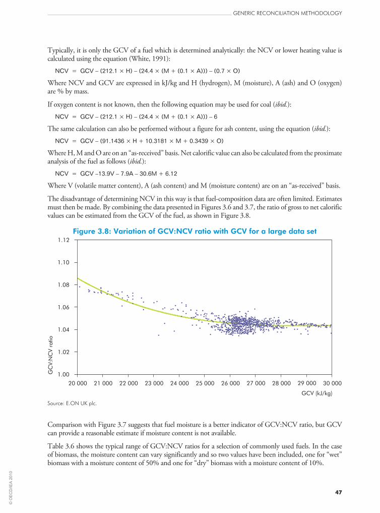
Typically, it is only the GCV of a fuel which is determined analytically: the NCV or lower heating value is calculated using the equation (White, 1991):

NCV = GCV – (212.1 × H) – (24.4 × (M + (0.1 × A))) – (0.7 × O)

Where NCV and GCV are expressed in kJ/kg and H (hydrogen), M (moisture), A (ash) and O (oxygen) are % by mass.

If oxygen content is not known, then the following equation may be used for coal (ibid.):

NCV = GCV – (212.1 × H) – (24.4 × (M + (0.1 × A))) – 6

The same calculation can also be performed without a figure for ash content, using the equation (ibid.):

NCV = GCV – (91.1436 × H + 10.3181 × M + 0.3439 × O)

Where H, M and O are on an “as-received” basis. Net calorific value can also be calculated from the proximate analysis of the fuel as follows (ibid.):

NCV = GCV –13.9V – 7.9A – 30.6M + 6.12

Where V (volatile matter content), A (ash content) and M (moisture content) are on an “as-received” basis.

The disadvantage of determining NCV in this way is that fuel-composition data are often limited. Estimates must then be made. By combining the data presented in Figures 3.6 and 3.7, the ratio of gross to net calorific values can be estimated from the GCV of the fuel, as shown in Figure 3.8.

Figure 3.8: variation of GCv:NCv ratio with GCv for a large data set

1.00

1.02

1.04

1.06

1.08

1.10

1.12

20 000 21 000 22 000 23 000 24 000 25 000 26 000 27 000 28 000 29 000 30 000

GCV (kJ/kg)

GC

V:N

CV

ratio


Comparison with Figure 3.7 suggests that fuel moisture is a better indicator of GCV:NCV ratio, but GCV can provide a reasonable estimate if moisture content is not available.

Table 3.6 shows the typical range of GCV:NCV ratios for a selection of commonly used fuels. In the case of biomass, the moisture content can vary significantly and so two values have been included, one for “wet” biomass with a moisture content of 50% and one for “dry” biomass with a moisture content of 10%.


47

© O

EC

D/IE

A 2

010

Table 3.6: Typical GCv:NCv ratios for various fuels

Fuel Typical GCV:NCV ratio

“Wet” biomass 1.250

Lignite 1.159

Natural gas 1.108

“Dry” biomass 1.091

Sub-bituminous coal 1.074

Heavy fuel oil 1.059

Light fuel oil 1.058

Bituminous coal 1.045

Anthracite 1.025


The carbon-to-hydrogen ratio of fuels can be determined from the ultimate analysis. However, such analysis are not performed routinely. The following formula, based on work by Seyler-Dulong (White, 1991), enables an estimate of the carbon content of coal from its moisture, ash and volatile content, and GCV. These parameters are generally known from the proximate analysis or can be estimated.

carbon % (ar) = ((0.0014081 × GCVdaf) – (0.21633 × VMdaf) + 43.4) × (100 – M – A) / 100

Where GCVdaf is expressed in kJ/kg and VMdaf, M and A as % by mass.

Figure 3.9: dry, ash-free volatile matter as an indicator of carbon:hydrogen ratio for a large data set

0

5

10

15

20

25

30

25 30 35 40 45 50 55

Volatile matter (%daf)

Carb

on:h

ydro

gen

ratio


Figure 3.9 shows empirically that the dry, ash-free volatile content of a coal can provide a good indicator of its carbon-to-hydrogen ratio, and therefore its carbon intensity, assuming its calorific value is known. Table 3.7 shows typical carbon:hydrogen ratios for a variety of fuels.


48

© O

EC

D/IE

A 2

010

Table 3.7: Typical carbon:hydrogen ratios for various fuels

Fuel Typical C:H ratio

Anthracite 32.6

Bituminous coal 15.2

Sub-bituminous coal 14.9

Lignite 14.0

Biomass 8.3

Heavy fuel oil 7.5

Light fuel oi 7.3

Natural gas 3.1


These empirical relationships, based on commonly known fuel properties, provide a basis for generic fuel-quality corrections to plant efficiency and specific CO2 emissions data. For non-condensing plant designs, the quantity of fuel required is related to its net calorific value. The carbon released in providing that heat is related to the C:H ratio, and the overall carbon intensity can be related to the GCV:NCV ratio and the C:H ratio of the fuel. The C:H ratio, the gross calorific value of hydrogen relative to carbon (141.886 MJ/kg / 32.808 MJ/kg = 4.325), and the GCV:NCV ratio, which could be arbitrarily termed the “fuel carbon intensity factor”, can be combined to compare a range of different fuels without any need for detailed knowledge of fuel composition.

fuel carbon intensity factor = GCV / NCV / (1 + 4.325 / C:H)

This is important when considering the specific CO2 emission of a process. If this value is normalised with reference to one of the fuels of interest a “relative fuel carbon intensity factor” can be derived. This factor allows easy comparison of the impact of fuel quality on specific CO2 emissions (effectively comparing the quantity of carbon burned for a given net heat input). These factors are shown calculated in Table 3.8 using information from tables above.

Table 3.8: relative carbon-intensity factors for various fuels(with bituminous coal as the reference case)

Fuel GCV:NCV C:H ratioFuel carbon

intensity factor

Relative fuel carbon intensity

factor

Anthracite 1.025 32.58 0.90 1.11

Lignite 1.159 13.97 0.88 1.09

Sub-bituminous coal 1.074 14.86 0.83 1.02

Wet biomass 1.250 8.32 0.82 1.01

Bituminous coal 1.045 15.22 0.81 1.00

Dry biomass 1.091 8.32 0.72 0.88

Heavy fuel oil 1.059 7.49 0.67 0.83

Light fuel oil 1.058 7.32 0.66 0.82

Natural gas 1.108 3.06 0.46 0.56



49

© O

EC

D/IE

A 2

010

It should be noted that this calculation is based on fuel properties and excludes the effects of plant design and performance, and the contribution of fuel production and supply on CO2 emissions. It also excludes the potential impact of, for example, ash quantity, ash fusion properties and fuel reactivity variations on boiler performance (although these can be largely managed through appropriate design and operation). Literature suggests that, compared to bituminous coal-fired plants, the efficiencies of plants firing sub-bituminous coal and lignite are respectively about 5% and 10% lower on a NCV, net output basis. For example, a plant with steam conditions and cooling system suitable for achieving an efficiency of 45% with hard coal might only deliver 42.8% with sub-bituminous coal and 40.5% with brown coal or lignite on a NCV, net output basis.

Figure 3.10 illustrates the more general impact of coal moisture on overall unit performance when the combined effects of latent heat (GCV-NCV differential), alteration of flue gas dew point temperature (due to moisture in gas) and additional fan power (due to additional mass and volume flows) are taken into account. It should be noted that this has been derived for a relatively low-ash coal and efficiencies could well deteriorate more for high-ash coals. It should also be recognised that the curves will be affected by the sulphur content of the coal and its impact on dew point temperature (see below).

Figure 3.10: Approximate influence of coal moisture on plant efficiency

26

28

30

32

34

36

38

40

42

44

46

5 10 15 20 25 30 35 40 45 50 55 60


Unit

effic

iency

(%)

NCV (LHV) basis

GCV (HHV) basis


New technologies for lignite-fired boilers address the effects of moisture by recovering heat lost from the steam cycle to dry incoming fuel. While this improves the efficiency of the plant, and leads to lower fuel consumption, it does not change the fact that lignite requires energy to dry it prior to combustion. For example, the low-grade heat used to dry lignite could be put to alternative use, such as district heating, if bituminous coal were used instead in the same boiler. Lignite is, however, a competitive and abundant fuel; its use is likely to continue in certain regions, and fuel drying will secure more output and lower emissions.

In the case of blended fuels, co-firing or the use of secondary fuels, the factors described above can be combined pro-rata, weighted by their gross heat contributions. Any carbon offset associated with the use of biomass fuels would need to be considered separately.


50

© O

EC

D/IE

A 2

010

Steam conditions

As described above, the steam cycle boundary conditions have a significant impact on overall plant efficiency. In this respect, the temperatures and pressures of the main and reheat steam are major design considerations. Figure 3.11 provides a means to correct the heat consumption of single reheat cycles operating with different main steam and reheat conditions (all other factors being equal). This diagram does not extend to cycles using supercritical steam conditions of 350 bar, 700/720 °C which should offer heat rate improvements in the order of 14%. Such cycles are currently being investigated in Europe under the AD700 project and in the USA by the DOE and EPRI.

Figure 3.11: Heat rate improvement with main steam and single reheat temperature at different main steam pressures

593/621 Co

593/593 Co

565/593 Co

565/565 Co

538/565 Co

538/538 Co

9

8

7

6

5

4

3

2

1

0Heatra

teim

pro

vem

ent(%

)

150 200 250 300 350

Rated main steam pressure (bar)(figures on curve are main and reheat steam temperatures

oC)

Single reheat

source: Henderson (2004) after logan and nah (2002).

Using the curves above, an efficiency correction factor19 can be established based on superheat temperature, superheat pressure, the ratio of reheat temperature to superheat temperature and reference conditions of 160 bar, 565/565 °C for a single reheat cycle:

correction = 0.4292 + (0.000403 × P) – (3.5 × 10–7 × P2) + (0.000637 × M) + (0.1548 × R / M)

Where P is the main steam pressure (bar), M is the main steam temperature (°C), and R is the steam reheat temperature (°C).

This relationship should only be considered valid for the data in Figure 3.11. Steam conditions are a key design parameter for any power plant; once chosen, they largely determine the efficiency performance that can be expected at a particular site using a specified fuel. It is not proposed that corrections be made for steam conditions within the context of general efficiency reconciliation, unless it is specifically of interest.

19 corrected reference efficiency (%) = uncorrected as-reported efficiency (%) × efficiency correction factor


51

© O

EC

D/IE

A 2

010

Reheat stages

Plants using reheat cycles are more efficient than those without reheat, and two stages of reheat are normally even more efficient, assuming its use can be justified economically. Non-reheat cycles were used in the past, but are not usually found in modern plants. Correction factors for efficiency, based on number of reheat stages, are shown in Table 3.9, assuming other factors remain constant. The reference case is one stage of reheat. Figure 3.12 illustrates the potential benefits of double reheat with higher steam conditions.

Table 3.9: efficiency correction factors for number of reheat stages

Reheat stages Correction factor

None 0.900

Single 1.000

Double 1.015

Figure 3.12: Heat rate improvement at different main steam pressure, with increasing main steam and double reheat temperatures

9

8

7

6

5

4

3

2

1

0

150 200 250 300 350

593/621/621 Co

593/593/593 Co

565/593/593 Co

565/565/565 Co

538/565/565 Co

538/538/538 Co

Double reheat

Single reheat538/538 C

o

Heatra

teim

pro

vem

ent(%

)

Rated main steam pressure (bar)(figures on curve are main and reheat steam temperatures

oC)

source: ge Power generation (1996). reprinted by permission of the publisher. © ge energy, 1996.

Cooling-water system

Seawater cooling generally allows the highest efficiencies to be achieved, especially for power plants adjacent to cool seas using once-through cooling systems. Once-through designs using river water also perform well, although the cooling-water temperatures tend to be higher. Constraints on water abstraction and use mean that it is common for inland stations to use closed-circuit cooling systems with cooling towers. These systems run with a higher cooling-water temperature in the recirculation system which lowers performance. In cases where water is scarce, dry-cooling systems may be used. Such systems are rarely employed because they result in a very significant efficiency penalty. In Table 3.10, corrections are proposed, based on the type of cooling system employed. The reference case is assumed to be an inland station with a wet cooling-tower system.


52

© O

EC

D/IE

A 2

010

Table 3.10: efficiency correction factors for type of cooling system employed

Cooling system type Correction factor

Seawater (once-through) 1.024

River water (once-through) 1.015

Closed-circuit, wet tower 1.000

Closed-circuit, dry tower 0.952

Forced-ventilation cooling towers may be capable of achieving lower condenser pressures than natural-draught towers. However, their use offers no clear advantage after the associated power consumption has been taken into account, so no correction is proposed for forced-ventilation towers.

Ambient temperature

Cooling-water temperature will tend to be influenced by ambient temperature. Changes to ambient temperature will affect the boiler air to hot gas temperature rise, boiler radiation losses and fan power. The reducing boiler heat losses as ambient temperature increases will tend to be offset by worsening cooling system performance. For an ambient air temperature rise of say 10 °C, around 0.5% less fuel would be required to achieve the same hot gas temperature in the boiler. The impact of such a change in ambient temperature on cooling water would likely result in a 2% increase in heat rate – a net effect of +1.5%. It is therefore proposed that, where required, a nominal correction to heat rate of +0.15% per 1 °C increase in ambient temperature should be applied.

Ambient conditions can significantly affect the performance and load capability of gas turbines. This may be relevant for hybrid plants firing both natural gas and coal. Ambient temperature and pressure may also affect the performance of any plants employing air separation units for oxygen production.

Flue gas cleaning

Emissions control, such as flue gas treatment equipment, generally has an adverse impact on plant efficiency and CO2 emissions (unless captured). From industrial experience, the heat-rate correction factors in Table 3.11 can be applied to “as-reported” plant efficiencies to account for the impact of commercial pollution control technologies.20

Table 3.11: Heat rate correction factors for different gas treatment technologies

Technology employed Correction factor

Wet FGD (compared with no FGD) 1.0200

Dry FGD (compared with no FGD) 1.0100

LNB and OFA 1.0050

SCR 1.0050

Bag filter (instead of ESP) 1.0050

SNCR 1.0025

notes: esP: electrostatic precipitators; fgd: flue gas desulphurisation; lnb: low-nox burners; ofa: over-fire air; scr: selective

catalytic reduction of nox, sncr: selective non-catalytic reduction of nox.

20 corrected reference efficiency (%) = uncorrected as-reported efficiency (%) / heat-rate correction factor


53

© O

EC

D/IE

A 2

010

54


Although not currently employed, a similar correction can also be made for CO2 capture. This can be integrated into the calculations in a similar way to FGD, with a direct heat-rate penalty component and a second component associated with the CO2 removal rate. In the case of applying CO2 capture to a pulverised coal combustion plant, the heat-rate correction factor could be in the region of 1.2, based on current knowledge of the technology.

Fuel sulphur content and dew point

The fuel sulphur content will have some impact on the minimum flue gas temperature to avoid dew-point conditions and formation of corrosive acids. Very approximately, the minimum operating temperature to avoid the dew point for bituminous coals with average moisture can be related to sulphur and moisture content. This can then be converted into a change in boiler sensible heat loss.

To avoid the acid dew point, a flue gas temperature rise of 1 °C per 0.2% sulphur in coal, above a nominal level of 1% sulphur (dry basis), can be assumed; with a further 1 °C per 5 percentage point rise in the as-received moisture content. The recommended reference moisture level is 12%. This can be translated into a heat rate increase of approximately 0.3% per 1 percentage point change in sulphur, in addition to a 0.01% increase in heat rate per 1% moisture. Below 1% sulphur, the dew-point correction should only take account of moisture since power plants are rarely designed to accept only fuels of less than 1% sulphur. The true dew point relationships are complex, but the proposed approach provides a simple basis on which to make approximate corrections.

These corrections are distinctly separate from the impact of installing FGD to control sulphur dioxide emissions and the direct impact of moisture on fuel calorific value and sensible heat losses. The effect of fuel moisture is considered in Figure 3.10 and the impact of desulphurisation in Table 3.11.

Some power plants may use a low-sulphur coal, but then inject SO3 to maintain electrostatic precipitator performance. In such situations, the potential benefits of reducing flue gas temperature when using low-sulphur coal may not be realised, since dew-point problems could persist as a result of the SO3 injection. The SO3 effectively raises the dew-point temperature back towards that found with a higher-sulphur coal.

Fuel ash content

Coal ash, an inert diluent, is generally a nuisance: higher levels of ash require the delivery and processing of more coal and the collection and transfer of more ash. The presence of more ash also requires the use of more soot blowing to remove ash deposits in the boiler furnace and convective heat transfer sections to maintain good heat transfer. Ash discharged from the furnace bottom and removed from the flue gas takes with it a quantity of sensible heat. There is therefore an additional energy penalty associated with the use of high-ash fuels, irrespective of their other properties. Firing high-ash coal on a plant not designed for such fuel can create performance problems (mainly associated with boiler heat transfer), although plants that are designed for these fuels can operate well and with high efficiency.

A small ash correction factor could be applied, where appropriate, proportional to the ash content. A figure of +0.03% on heat rate per 1 percentage point dry ash is proposed, based on a reference ash level of 12%. On this basis, the difference in heat rates between a plant using 8% dry ash fuel and an otherwise identical plant using 18% dry ash fuel would be 0.3%.

Auxiliary power

Auxiliary power requirements differ for various reasons, including the use of:

• electric driven boiler feed-water pumps;

© O

EC

D/IE

A 2

010

55


• higher boiler pressures;

• different designs of coal pulverising plant;

• fuels with different densities, and hence volumes;

• different flue gas treatment technologies;

• modern motors and flow controls; and

• compressed air soot blowers.

Operation at part load, or with many start-ups and shutdowns, will increase the relative auxiliary power requirement. There are also differences in how auxiliary power is accounted for, since even large plant items, such as condenser cooling-water pumps and boiler feed-water pumps, can usually be driven from the station supplies (imported power) or the unit supplies (generated power). Such differences in power supply arrangements can influence efficiency significantly when calculated on a unit basis, but will have no effect on efficiency expressed on a whole-plant basis. This, and the inclusion of common plant energy requirements associated with fuel and ash handling, are good reasons to adopt a whole-plant efficiency evaluation basis.

Main boiler feed-water pumps are typically steam driven, with electric start-up and stand-by pumps. Although electric feed-water pumps can be used, their power consumption needs to be evaluated carefully to understand the impact on plant performance compared with steam-driven pumps. Overall efficiency is likely to be similar for either option, assuming that the plant is designed for one or the other from the outset. However, if a plant is designed for a steam-driven pump and then operates with electric pumps, this is generally detrimental to plant efficiency, since changes to the steam system affect both feed-water heating and steam flows to the main turbine and boiler reheater.

Other changes to auxiliary power are either insignificant or are already taken into account by corrections proposed elsewhere in this report. Typically, works power may range from 2.5% to as much as 8% of a unit’s generated power, with high-end values applying to high-pressure supercritical units with electric-driven main boiler feed-water pumps, and low-end values to low-pressure units with steam-driven main boiler feed-water pumps and vertical-spindle coal mills.

Feed-water heating, reheater pressure loss and reheat spray

There are some key plant design parameters which influence plant performance, such as the number and position of feed-water heaters (which influence boiler feed-water temperature), the design pressure loss across the reheater and the quantity of reheat spray required. These are inherent to a power plant’s design and therefore require no correction, since it is largely such design differences that are being assessed when comparing the performance of a particular plant against best practice. The same argument applies to the design steam temperature and pressure.

Generator power factor

Generator power factor has an impact on losses and heat rate. However, this effect is considered to be too small to justify correction here. Such a correction could be added, if required, but would require the submission of operational power factor information for each plant and a justification for why a correction might be needed.

Number of units and unit capacity

There are generally good practical and economic reasons to employ more than one power generation unit on a particular site and to build large units. Economies can be made by sharing facilities and resources (e.g. coal and ash plant, staff and spares holdings), and through the relatively lower cost of larger units of a given design.

© O

EC

D/IE

A 2

010

56


Overall, the efficiencies of higher capacity units are better than those of smaller units, largely because they are more modern. Early power generation units were very small by today’s standards and newer units have progressively increased in both size and technological advancement. If smaller generating units were installed today, then they would be very much more efficient than older units of the same size – it is important to differentiate between the impacts of plant age and plant size.

While larger plant will tend to have higher efficiencies, there are insufficient data available at this time to justify a reliable correction for plant size. Furthermore, it is considered that the efficiency impact of installing multiple small units, instead of a single large unit, has a negligible impact on plant efficiency, even though the impact on overall plant economics could be very significant.

Boiler radiation and “unaccounted” losses

Boiler radiation and “unaccounted” losses are usually agreed with the boiler supplier, and are often determined by reference to standard methods such as the charts by the American Boiler Manufacturers Association (ABMA). The losses are fairly constant when the plant is in operation, but become a relatively larger proportion of the heat input as load is reduced. Smaller plants, with larger surface-to-volume ratios, suffer more from these losses, although losses become progressively less sensitive to plant size as size increases. Large modern units would be expected to have losses of around 0.5% at average load, but this could rise to 3% for a small older unit (<100 MW) with low average operating load. For the purposes of this evaluation, it is assumed that the boiler radiation and unaccounted losses are reflected in the whole-plant efficiency such that changes in these losses with load are taken into account by whole-plant load correction factors. Related to these losses, however, is whether the plant is designed with or without a main building enclosure and the ambient environment in which it operates. Typically, for temperate climates, the losses might be expected to be 50% higher for external plant. It is therefore proposed that the reference case should be an indoor plant, with a small generic correction of +0.375% on heat rate applied to external plant – irrespective of plant size and average load.

Excess air and unburned carbon

Excess air and unburned carbon in ash are largely operational issues. Although they directly affect boiler thermal losses, these are controllable losses that can be managed at the site level; plant efficiency corrections are not required.

Controllable losses

In any operating power plant, peak performance may no longer be reached because of the condition of the plant. In some cases, a step change in performance may be observed. For example, a plant may be called on to operate with stand-by equipment in service, or may be configured in an abnormal way (e.g. with feed-water heaters out of service). Other effects may be more gradual and related to leakage, wear, lack of adjustment or control and instrumentation problems. Such losses can generally be rectified, but degrade the efficiency of the plant if left unchecked. They are difficult to predict, although they are generally higher as a plant approaches its routine overhaul. It is proposed that a blanket allowance of +1% on heat rate is made, where justified, to account for a “reasonable” time-averaged level of controllable losses compared to ideal performance.

© O

EC

D/IE

A 2

010

57

efficiency outlook for Power generation from coal

4. eFFiCieNCy ouTLooK For PowerGeNerATioN FroM CoAL

The need for energy, together with the economics of producing and supplying that energy to the end user, are central considerations in power plant investment decisions and operating strategies. Inevitably, there will be a point at which higher efficiency and lower emissions come at a cost which cannot be justified. Where economic and regulatory conditions exist which shift this balance consistently in favour of higher efficiency and lower emissions, improvements become a normal part of running a competitive business. The trend over time has been towards improved power plant performance.

Worldwide coal-fired power plant efficiency averaged 35.1% in 2007, compared with 33.5% in 1971.21 Figures 4.1, 4.2, 4.3 and 4.4 illustrate the evolution of efficiency in countries where coal is used widely for electricity generation and heat supply. This top-down assessment is based on annual coal consumption and electricity supply data collected by the IEA. The annual data (dashed lines) are smoothed by using five-year moving averages to show long-term trends (solid lines). Fuel energy input is on a net calorific value (NCV) or lower heating value (LHV) basis, while electricity output is on a gross basis (i.e. at the generator terminals, before any deduction for on-site electricity use), each being the basis adopted by the IEA for reporting energy statistics.22 Heat supply is based on the quantity of heat supplied under commercial arrangements; the gross-net concept has no meaning for heat supply. Efficiency is calculated after correcting for heat supply using the methodology adopted by the EU.23 While this assessment allows comparison of coal-fired power generation efficiency at the national level, it does not allow performance comparisons to be made between individual plants; indeed, the IEA does not collect plant-level data.

Although drawing national comparisons is not the purpose of this report, some observations can be made on the four figures:

• The most rapid efficiency improvements have been seen during periods when large new coal-fired power plants were being built, for example in Japan, Korea and South Africa.

• In North America, much of the fleet of coal-fired power plants operating today was built during the 1960s, so efficiency performance has been largely unchanged over the last forty years. The availability of competitively priced indigenous coal and the need to retrofit pollution control equipment have not favoured efficiency improvements.

21 On a lower heating value, gross electrical output basis, after correction for heat supply. The average efficiency in 2007 is estimated to be 32.6% on a net output basis, assuming power plant own use of approximately 7%. The reported average efficiency would be lower if no correction were made for heat supply (see Figure 4.5).

22 Note that this report recommends that efficiency be reported on a fuel’s gross calorific value (GCV) or higher heating value (HHV) basis, and a net electricity sent-out basis.

23 See footnote 8.

© O

EC

D/IE

A 2

010

58


• In Europe, the trend of improving efficiency reflects the closure of older, less efficient coal-fired power plants, replaced either by new coal-fired plants or other energy sources for power generation such as natural gas, renewable sources and nuclear.

• Coal-fired power generation efficiency shows a gradual improvement in China as more new plants are built with improved performance.

• Countries which exploit poor quality coal for power generation are faced with lower levels of efficiency, for example in Australia and India. Many power plants in these two countries must also contend with high ambient temperatures and limited water supplies, both contributing to lower efficiency.

• The cogeneration of heat and power can improve efficiency, for example in Russia and Poland. However, this assumes that the heat supplied is used effectively.

Figures 4.1, 4.2, 4.3 and 4.4: evolution of coal-fired heat and power plant efficiency in selected countries (annual data and five-year moving averages)

15%

20%

25%

30%

35%

40%

45%

50%

55%

1960 1965 1970 1975 1980 1985 1990 1995 2000 2005

Canada

United States

1960 1965 1970 1975 1980 1985 1990 1995 2000 2005

South Africa

Russia

China

India

1960 1965 1970 1975 1980 1985 1990 1995 2000 2005

Germany

Poland

Italy

United Kingdom

15%

15%

15%

20%

20%

20%

25%

25%

25%

30%

30%

30%

35%

35%

35%

40%

40%

40%

45%

45%

45%

50%

50%

50%

55%

55%

55%

1960 1965 1970 1975 1980 1985 1990 1995 2000 2005

Japan

Australia

notes: annual data are shown with dashed lines, five-year moving averages with solid lines. for russia, data are shown for 1990-1992, 1996 and 2005-2007. data for the intervening years show inexplicable efficiency improvements and may need revising.

source: iea databases.

The data reported in Figures 4.1 to 4.4 are not corrected for any of the factors discussed in Section 3. As such, it is a “raw” comparison that ignores the influences of uncontrollable variables on performance, such as ambient temperature.

The development of supercritical and ultra-supercritical steam cycles, with progressively higher steam temperatures and pressures, combined with modern plant design and automation, provide significant potential for further efficiency improvements and the mitigation of CO2 emissions when compared with existing coal-fired power plants. These improvements can be realised through the progressive replacement of existing assets with new plant designs that reflect best practices.

© O

EC

D/IE

A 2

010

59


Although a large number of supercritical and ultra-supercritical pulverised coal-fired power plants are currently under construction or planned, subcritical technology has continued to dominate recent build. However, with stricter requirements to limit CO2 emissions, the share of supercritical and ultra-supercritical plants should increase.

By far the largest energy loss from existing and future coal-fired power plants will remain the heat rejected from the steam cycle to the cooling water. The use of cogeneration or combined heat and power, along with district heating and cooling, has therefore received renewed interest in the light of requirements to improve energy efficiency and reduce specific CO2 emissions. However, the most significant potential to reduce CO2 emissions from coal-fired power plants will come through the application of CO2 capture and storage. Here, basic plant efficiency improvements will be a significant factor in ensuring the viability of carbon capture.

Figure 4.5 shows projections by VGB for the efficiency of and emissions from coal-fired power generation by 2020. With proper policy and financial support for demonstration, by 2015 the net efficiency of state-of-the-art units firing hard or bituminous coal could reach 50% (LHV, or around 48% HHV) at plants without CO2 capture and storage. For lignite-fired plants, these figures will be up to five percentage points lower depending on the moisture content of the coal, but that can be improved if developments in efficient coal-drying technology are successful, using either waste heat or low-grade steam.

Figure 4.5: efficiency improvement potential at hard coal-fired power plants

CO

em

issi

ons

per

kW

h2

2010 2020 Time

-21%

-33%

-40%

-90%

Averageworldwide

EuropeanUnion

State-of-the-arttechnology

Steam power plant700 C technology

o

CCS technologybut:efficiency loss7 to 12% points

CO

reduct

ion

2

Efficiency

CO2 emissions

Fuel consumption

30%

38%

45%

about 50%

1 116 g CO /kWh2

881 g CO /kWh2

743 g CO /kWh2

669 g CO /kWh2

480 g coal/kWh

379 g coal/kWh

320 g coal/kWh

288 g coal/kWh

source: vgb (2009). reprinted by permission of the publisher. © vgb Powertech e.v., 2009.

CO2 capture will impact significantly on the efficiency of both existing and future plants. At the current state of technology, units retrofitted with capture would suffer a decrease in efficiency of up to 12 percentage points, and consume perhaps 20% to 30% more fuel per unit of electricity supplied. While a concept of what constitutes “capture-ready” exists for new power plants, it may not be economic or technically viable to retrofit existing pulverised coal plants with CO2 capture, especially at smaller units. Refurbishments will often be necessary to improve efficiency at existing plants before CO2 capture retrofits can be contemplated. If 40% efficiency were to be considered the cut-off for CO2 capture retrofit, around 10% of the world’s

© O

EC

D/IE

A 2

010

current coal-fired capacity would be suitable for CCS.24 Even then, and assuming a route to storage, case-by-case analyses would be needed to assess whether existing control systems can be safely adapted and whether the large steam requirement of CO2 capture equipment can be sensibly supplied from these existing plants.

Owing to the loss of efficiency, retrofitted units will deliver less power; additional new capacity would likely be needed to offset this loss. Based on new-build information, project proposals and forecasts it appears that while the majority of future plants will be either supercritical or ultra-supercritical, with an efficiency above 40%, subcritical units will still have a significant market share. By 2030, up to half of the fleet might be considered suitable for CCS retrofit when necessary, while most of the remaining plants would require either upgrading to deliver high efficiencies or total replacement.25 Further work is needed to better define the future potential for CCS retrofit at coal-fired power plants.

24 Estimate using IEA Clean Coal Centre CoalPower5 database. Of the 7 173 units listed in the database, the individual efficiencies of a sample comprising 4 396 units (with a total capacity of 1 074 GW) has been estimated from available operating parameters. Of these units, 255 units (with a total capacity of 118 GW) are estimated to have an efficiency of greater than 40%.

25 Estimate from supercritical coal-fired power plants listed in Platts UDI World Electric Power Plants Database 2009 and analysis presented in IEA World Energy Outlook 2009.

60

efficiency outlook for Power generation from coal©

OE

CD

/IE

A 2

010

61

conclusions and recommendations

5. CoNCLuSioNS ANd reCoMMeNdATioNS

The major conclusions and recommendations of this report build on those presented to the G8 Hokkaido Summit in July 2008 (IEA, 2008). These are summarised in this section, before a discussion of the way forward.

5.1 IEA recommendations to the 2008 G8 Summit

Coal is the least costly and most accessible fuel for some of the most dynamic developing economies. Its use at coal-fired power plants accounts for over 28% of global CO2 emissions, a share that is rising. An absolute priority is to enhance plant efficiency, which can significantly reduce CO2 emissions and the volume of coal consumed. Available technology can deliver fuel savings of 50%.

Worldwide coal-fired power plant efficiency averages around 33% (LHV, net output). Implementation of the suggested measures from IEA work carried out in support of the G8 Gleneagles Plan of Action could result in the replacement of some 300 GW and retrofit of some 200 GW of older coal-fired power plant capacity, while ensuring that all new plants are state-of-the-art. This could, if fully implemented, lead to a reduction of up to 1.7 Gt per annum of CO2 emissions – which is roughly one-quarter of annual CO2 emissions from coal-fired heat and power production – and a reduction in coal consumption of at least 0.5 Gt per annum.

To improve the operating efficiency of the global fleet of coal-fired power plants – and thereby significantly reduce CO2 emissions – the IEA recommends that governments focus on the following policy approaches:

• New coal-fired power plants should be >40% efficient.26 Governments should look to replace by 2020 those coal-fired power plants built over 25 years ago and <300 MW. All other coal-fired power plants should be assessed for upgrading or replacement to achieve around 40% efficiency.

• International co-operation, training and financing mechanisms should be focussed on achieving the above best-practice efficiency objectives in the design, operation and maintenance of coal-fired power plants and electricity grids.

• The development and demonstration of those technologies that target higher efficiency at coal-fired power plants should be accelerated. For example, advanced materials, coal cleaning and drying, co-generation of heat and power, and more efficient CO2 capture technologies all need to be deployed.

In addition to these efficiency improvements, the deployment of CO2 capture and storage (CCS) technology is vital. The aim of reducing CO2 emissions by 50% by 2050 implies that virtually all coal-fired power plants will need CCS by then (including some under construction now). Based on IEA recommendations, G8 governments strongly support the launching of twenty fully integrated industrial-scale CCS demonstration projects globally, with a view to beginning broad deployment of CCS by 2020. The IEA further recommends

26 On a higher heating value, net electrical output basis. On a lower heating value basis, the figure is approximately 42%.

© O

EC

D/IE

A 2

010

62


that any developer of a new coal-fired power plant should consider now what might be required to retrofit CCS. In 2009, at the request of G8 leaders, the IEA launched a CCS technology roadmap that presents a detailed scenario for the deployment of CCS technologies, from a handful of demonstration projects to over three thousand projects by 2050 (IEA, 2009). The contribution of CCS to reducing global emissions under this scenario is significant: by 2050, CCS contributes almost one-fifth of the necessary emissions reduction to achieve stabilisation of atmospheric GHG concentrations in the most cost-effective manner.

5.2 Reporting efficiency performance

An understanding of the technical potential to improve efficiency is key to developing leading-edge technologies, implementing policies to encourage their widespread adoption and taking corporate investment decisions that see them deployed. Yet, the factors discussed in this report have illustrated how the same level of plant performance can be described by a confusingly wide range of efficiency values, depending on the bases used for their calculation and reporting. For example, quoted efficiencies of new plants operating at design conditions cannot be compared with efficiencies of typical plants operating under constrained or off-design conditions.

At present, there is no common standard for collecting and compiling coal-fired power plant efficiencies or specific CO2 emissions. Hence, there is no basis to compare the operational performance of power plants or to identify the potential for improvements. A means should be established to compare the performance of individual plants with best-practice performance.

Unfortunately, defining a new comprehensive methodology to rationalise plant efficiency reporting is not a practical proposition given the many different reporting bases and assumptions already in use around the world. Instead, a range of approximate corrections is proposed, requiring only limited information that can be collected even where the detailed bases of the original calculations are not known. Average figures, reported over a timescale of one month or more, will be inherently more reliable, reflecting the actual efficiency achieved more accurately than design values, performance guarantees or short-term tests under ideal conditions. The corrected data can then be compared with data for plants adopting best practices.

Care still needs to be taken to distinguish between real design constraints and controllable variables; applying corrections for every variable would ultimately lead to all plants appearing to have the same efficiency. This report has described a calculation methodology and estimated correction factors to reconcile performance data. In the context of evaluating overall plant efficiency and specific CO2 emissions, the errors introduced using this approach will be small compared to the differences in power plant efficiencies between typical plants and state-of-the-art ones, and between current and future potential. The approach outlined may not therefore be the most accurate, but forms a pragmatic and practical means of comparing plant efficiencies reported from different sources.

5.3 Improved collection of performance data

An essential part of sound policy development is the rigorous analysis of information which should be internally consistent and verifiable. Reliable power plant operating information is not easy to obtain, whether on a unit or whole-plant basis, particularly efficiency-related information such as coal quality, coal consumption and electricity generation. It is therefore proposed that an international database of annual average coal-fired power unit operating information should be established for the purposes of determining, monitoring, projecting, reporting and comparing coal-fired power plant efficiencies and specific CO2 emissions. Such a database could be maintained by the IEA Energy Statistics Division or by the IEA Clean Coal Centre Implementing Agreement (IEA CCC) as an extension of its existing CoalPower5 database of world coal-fired power plants.

© O

EC

D/IE

A 2

010

63


The regular updating of such a data-collection system would require manpower resources in addition to those that are currently employed to maintain the IEA CCC database. Although the general concept and outline of such a scheme is proposed in this report, the specific arrangements for data submission, processing and access would require further discussion and agreement with IEA member countries and non-member countries.

For such a system to work, there must be a clear responsibility on plant operators to submit data, rather than on the database operator to collect it. Participating countries could provide the required data through national government bodies, collected from operators of power plants above a defined minimum thermal capacity of say 50 MWth. These new reporting requirements would, in most cases, only require minor changes to existing reporting mechanisms, and the extent of data required on an annual basis would not be onerous. There would, however, be a fundamental requirement for every plant to monitor total energy input and output over the course of each year. Although this is standard practice for most plants, there may be some installations where additional monitoring equipment or procedures will be required.

Regional coverage of the scheme is a matter for further consideration. Clearly, the benefits of increasing the efficiency of the fleet of coal-fired power plants will be greatest in countries and regions with the largest demand and potential for investment, including China, North America, the European Union, India and Russia. However, the benefits of such a scheme would be evident in any country or region in which its implementation is possible.

Since most governments already collect energy data for statistical purposes, it should be relatively simple to extend systems already in place. Governments would need to decide on whether the availability and provision of such data should be mandatory for plant operators. They would also need to reach agreement on whether information should be published on a unit, plant, company or national basis, and on any criteria for exclusion. It may be that more detailed, unit-specific data could be collected for confidential use.

5.4 Performance benchmarking

In order to be useful in its underlying aim of encouraging best practice in coal use and understanding the potential for further improvement, an agreed view of best-practice performance would be needed. This should reflect efficiency and specific CO2 emissions at a number of exemplary coal-fired power plants, covering different plant designs and operating conditions. These best-practice performance figures may then be used as benchmarks, providing a basis for participating countries to consult with industry to determine appropriate future development strategies that reflect regional constraints and objectives. It should be recognised that the most efficient plant may not necessarily be the most economic plant to build, own and operate, or provide the best long-term security of supply. A better understanding of plant performance allows decision makers to better address the compromises that must be made.

5.5 The way forward

Policy makers must reflect on what steps are now needed to improve the overall efficiency of power generation from coal. This report presents the tools for analysis and makes recommendations on how to use these tools to compare performance. This will allow poorly performing plants to be identified, wherever they are located. The costs and benefits of refurbishing, upgrading or replacing these plants can be estimated as the first stage in developing new policies that would encourage greater efficiency. The prize is large: some estimates suggest that 1.7 GtCO2 could be saved annually. However, securing this reward would demand a major realignment of national energy and environmental policies, a realignment that may be less politically acceptable than allowing old, inefficient coal-fired power plants to continue running, in the hope that they will eventually fade away. Given that there appears to be no prospect of meeting global electricity demand without coal, governments must implement policies that respond more proactively to the growing use of coal, rather than wishing it away. Monitoring the efficiency of power plants and targeting those that perform poorly would be a step in that direction.

© O

EC

D/IE

A 2

010

69

ACroNyMS, ABBreviATioNS ANd uNiTS27

ABMA American Boiler Manufacturers Association

AGEB AG Energiebilanzen e.V.

AGO Australian Greenhouse Office

ar as-received (coal)

ARE Agencja Rynku Energii S.A. (Energy Market Agency, Poland)

ASME American Society of Mechanical Engineers (US)

ASTM American Society for Testing and Materials (US)

AUD Australian dollar

bar unit of pressure (105 Pa)

BERR Department of Business, Enterprise and Regulatory Reform (UK)

BGR Bundesanstalt für Geowissenschaften und Rohstoffe (Federal Institute for Geosciences and Natural Resources, Germany)

BlmSchV Bundes-Immissionsschutzverordnung (German federal emission control regulation)

BS British Standard

BSI British Standards Institution (UK)

Btu British thermal unit

C carbon

°C degree Celsius (or centigrade)

CAAA Clean Air Act Amendments of 1990 (US)

CaCO3 calcium carbonate (limestone)

CCS carbon (dioxide) capture and storage

CEA Central Electricity Authority (India)

27 See unit converter at www.iea.org/stats/unit.asp.

acronyms, abbreviations and units©

OE

CD

/IE

A 2

010

70

acronyms, abbreviations and units

CEGB Central Electricity Generating Board (UK)

CEM continuous emissions monitoring

CEN Comité Européen de Normalisation (European Committee for Standardization)

CIAB IEA Coal Industry Advisory Board

CO2 carbon dioxide

CO2e carbon dioxide equivalent (of GHG)

CV calorific value (also known as heating value)

daf dry, ash-free (coal)

DECC Department of Energy and Climate Change (UK)

Defra Department for Environment, Food and Rural Affairs (UK)

DEHSt Deutsche Emissionshandelsstelle (German Emissions Trading Authority)

DFID Department for International Development (UK)

DIN Deutsches Institut für Normung e.V. (German Institute for Standardization)

DNV Det Norske Veritas (Norway)

DOE US Department of Energy

EC European Commission

EIA Energy Information Administration (US)

EPA US Environmental Protection Agency

EPRI Electric Power Research Institute (US)

ESP electrostatic precipitator

ESWG Efficiency Standards Working Group (Australia)

ETS EU Emissions Trading Scheme

EU European Union

FEPC Federation of Electric Power Companies (Japan)

FERC Federal Energy Regulatory Commission (US)

FGD flue gas desulphurisation

g gramme

G8 Group of Eight (Canada, France, Germany, Italy, Japan, Russia, UK, US)

gce gramme of coal equivalent

GCV gross calorific value

GE General Electric Inc.

GES Generator Efficiency Standards (Australia)

© O

EC

D/IE

A 2

010

71


GHG greenhouse gas

GIOS Główny Inspektorat Ochrony Środowiska (Chief Inspectorate for Environmental Pollution)

GJ gigajoule (109 joules)

GOST gosudarstvennyy standart Rossii (Russian national technical standard)

Gt gigatonne (109 metric tonnes or billion tonnes)

GWh gigawatt-hour (109 watt-hours)

GWP global warming potential (of a GHG)

GUS Główny Urząd Statystyczny (Central Statistical Office, Poland)

H hydrogen

HHV higher heating value

HR heat rate

HRSG heat recovery steam generator

IEA International Energy Agency

IEA CCC IEA Clean Coal Centre

IGCC integrated gasification combined cycle

I/O input/output (method of calculating power plant efficiency)

IPCC Intergovernmental Panel on Climate Change

IPPC Integrated Pollution Prevention and Control [Directive] (EU)

ISO International Organization for Standardization

IUPAC International Union of Pure and Applied Chemistry

K kelvin (unit of temperature)

KASHUE Krajowy Administrator Systemu Handlu Uprawnieniami (National Administration of the Emissions Trading Scheme, Poland)

KEMCO Korea Energy Management Corporation

KETEP Korea Institute of Energy Technology Evaluation and Planning

kg kilogram

kJ kilojoule (103 joules)

kWh kilowatt-hour (103 watt-hours)

lb pound (unit of mass)

LCPD EU Large Combustion Plants Directive

LHV lower heating value

LNB low-NOx burner

© O

EC

D/IE

A 2

010

72


LOI loss on ignition (of ash mass)

m3 cubic metre

mbar millibar (10-3 bar)

MCR maximum continuous rating

METI Ministry of Economy, Trade and Industry (Japan)

mg milligram

MJ megajoule (106 joules)

MMBtu million Btu

Mt million tonnes

MW megawatt (106 watts)

MWe megawatts electrical

MWh megawatt-hour (106 watt-hours)

MWth megawatts thermal

NCV net calorific value

NETCEN National Environmental Technology Centre (UK)

NETL National Energy Technology Laboratory (US)

NIST National Institute of Standards and Technology (US)

Nm3 normal cubic metre (of a gas)

NOx oxides of nitrogen

NPI National Pollution Inventory (Australia)

NTPC National Thermal Power Corporation (India)

OFA over-fire air (used in a boiler)

O/L output/loss (method of calculating power plant efficiency)

O&M operation and maintenance

Pa pascal (unit of pressure)

PC pulverised coal (also referred to as pulverised fuel)

pf pulverised fuel

PI pollution inventory (UK)

PLF plant load factor

PM10 particulate matter <10 μm

PTC Performance Test Codes (ASME)

Rosstat Federal State Statistics Service (Russia)

© O

EC

D/IE

A 2

010

73


SC supercritical (steam)

SCR selective catalytic reduction

SEB State Electricity Board (India)

SHR station heat rate

SNAP 97 Selected Nomenclature for Air Pollution (adopted in 1997)

SNCR selective non-catalytic reduction

SO sent-out (electricity)

SO2 sulphur dioxide

SO3 sulphur trioxide

STEP Station Thermal Efficiency Performance (CEGB, UK)

t metric tonne (1 000 kg)

tce tonne of coal equivalent

UK United Kingdom

UNECE United Nations Economic Commission for Europe

UNFCCC United Nations Framework Convention on Climate Change

URE Urząd Regulacji Energetyki (Energy Regulatory Office, Poland)

US United States

USC ultra-supercritical (steam)

VDI Verein Deutscher Ingenieure (Association of German Engineers)

VGB VGB PowerTech e.V., a European technical association for power and heat generation (formerly Verband der Großkraftwerks-Betreibe – Association of Large Power Plant Operators)

VM volatile matter (of coal)

WBCSD World Business Council on Sustainable Development

WRI World Resources Institute

© O

EC

D/IE

A 2

010

75

aPPendix i: understanding efficiency in a Power station context

APPeNdix i: uNderSTANdiNG eFFiCieNCyiN A Power STATioN CoNTexT

The following notes discuss the concepts and complexities of defining efficiency and some of the fundamental difficulties which may arise in efficiency analyses. They illustrate that the treatment of energy and efficiency is not as straightforward as it might initially appear, even before any of the more detailed technical considerations associated with process design, performance variability and measurements have been taken into account.

Energy supply chain

The assessment of performance, efficiency and emissions related to energy utilisation activities are complex and require constraining with identifiable system boundaries to enable a clear and consistent approach to be followed.

Figure i.1: Typical sequence of events in fuel utilisation

Carbon dioxide

Energy dissipation

ProductionENERGY

RESOURCEUtilisationConversionSupply Distribution NEED


© O

EC

D/IE

A 2

010

76


Consider a coal-fired power plant as an example. Fuel must first be sourced, mined, processed, shipped, delivered and converted into electricity or heat for distribution to the end user, who consumes the supplied energy to meet a particular need (Figure I.1). In terms of overall CO2 production and energy efficiency, it can be argued that it is actually the whole sequence of events, from sourcing the initial fuel to the energy service enjoyed by the end user that is important. The conversion efficiency of the power plant is only one element of a much bigger picture.

In order to assess power plant performance and specific CO2 emissions, it is necessary to concentrate on the conversion process. This does not mean that the other links in the energy chain should be ignored: they all have critical roles to play in energy conservation and environmental protection.

What is efficiency?

In general terms, efficiency is the output of a process compared to the input. It can, for example, be defined in terms of “economic efficiency”, “operational efficiency” or “energy efficiency”. Economic efficiency is essentially the specific cost of producing useful output, and tends to be the main driver behind shaping process plant design and operation. Although energy efficiency is considered in the analysis of economic efficiency, it is quite possible for plants with low energy efficiency to also have high economic efficiency. Operational efficiency is generally called “capacity factor” or sometimes “load factor” and measures the actual output from a process compared to the potential maximum output. This is less important in business terms than economic efficiency, but is still a major performance indicator. Energy efficiency is the efficiency indicator which is familiar to most people and is a measure of the useful energy from a process relative to the energy input. Strictly speaking, energy efficiency refers to the ratio of useful work output to the heat input, so it may be more correct to use “energy conversion efficiency” when considering mixed inputs and outputs which may be in different energy forms.

For power generation plant using fossil fuels, the inputs are typically electrical power and heat (i.e. chemical) energy and the outputs are electrical power and sometimes useful heat. Although energy efficiency is often expressed as a percentage, it is also frequently referred to as “heat rate”. Heat rate is the quantity of heat required to produce a given output and therefore a lower heat rate is more efficient and gives a higher percentage efficiency. The relationship most frequently used for heat rate and efficiency in respect of electrical power generation is:

efficiency = 3 600 / heat rate

Where heat rate is measured in kJ/kWh, MJ/MWh or GJ/GWh.

For example, a plant with a heat rate (i.e. heat consumption rate) of 9 000 kJ/kWh of output would have an energy efficiency of 40%. A 1% change in heat rate would change heat consumed by 1% but would only change the efficiency value by 0.4 percentage points. It is a common error to assume that a 1 percentage point change in efficiency is a 1% change in heat consumption and it is not unusual for sources of data which refer to and discuss efficiency to confuse these two measures.

Energy related analyses often refer to terms such as thermal efficiency, gross, net, isentropic efficiency, efficacy, exergy, emergy and other terms. It is worth clarifying these before considering process detail further.

“Thermal efficiency” is strictly defined as the useful output energy for a given quantity of gross input heat energy and is therefore subtly different from energy conversion efficiency, which might include both heat and power as inputs and outputs.

In thermodynamics, “exergy” is defined as a measure of the potential of a system to do work. In systems energetics, exergy has been defined as entropy-free energy. In thermodynamics, the exergy B of a system with respect to a reservoir is the maximum work done by the system during a transformation which brings it into equilibrium with the reservoir. Exergy analysis is used in the field of industrial ecology as a tool to both

© O

EC

D/IE

A 2

010

77


decrease the amount of exergy required for a process, and use available exergy more efficiently. The term was coined by Zoran Rant in 1956, but the concept was developed by J. Willard Gibbs in 1873. Rant also introduced the concept of “anergy”, which is the complementary part of the (heat) energy that cannot be converted into work.

Exergy efficiency is also called second-law efficiency because it computes the efficiency of a process taking the second law of thermodynamics into account. The energy E and exergy B balances of a process are:

Einput = Ein product + Eloss

andBinput = Bin product + Bloss + Bdestroyed

The efficiency h of the process may be described using the thermodynamic potentials E or B. Efficiency is the fraction of the potential that makes its way into the product.

The efficiency quoted by equipment suppliers is usually the energy conversion or first-law thermodynamic efficiency. This indicates how well the particular appliance converts one form of energy into another, but it does not indicate how the equipment compares to an alternative energy process. An example which can be used to illustrate the difference between energy conversion efficiency and exergy efficiency is the combustion of natural gas solely to heat water. While this has a high first-law efficiency, it has a low second-law efficiency, and wastes a large amount of high-temperature, high-quality energy to heat the relatively cold water. A combined heat and power system, with inherently higher exergy efficiency, uses the fuel to run a heat engine and then uses low-temperature waste heat for the water heating duty.

The new word “emergy” is a contraction of the term “embodied energy”. The need for this word arose because of an important difference in the way the two related disciplines of systems ecology and energy analysis were using the term “embodied energy”. The concept of embodied energy (i.e. the energy used up directly and indirectly in transformations to make a product or service) was given the name “emergy” and its unit defined as the “emjoule” or “emcalorie”. Other related properties, such as empower and emtropy also arise from the consideration of emergy. As a relatively recent innovation, there is still some ambiguity regarding its meaning and use, despite widespread use in the literature.

“Effectiveness”, generally referred to as the capability of producing an effect, is often used in relation to heat exchangers as a proxy for efficiency. The term “efficacy”, simply a measure of the ability to produce a desired amount of a desired effect, is also used in relation to efficiency. However, the focus of efficacy is the achievement of the desired effect, not the resources spent in achieving it. Based on these definitions, what is effective is not necessarily efficacious (the effect may be there, but not desired), and what is efficacious may not necessarily be efficient.

Another expression, used in the context of heat pump efficiency, is the “coefficient of performance”. The objective of a heat pump is to achieve the maximum amount of heat transfer, with the minimum amount of energy, leading to the erroneous description of its efficiency as greater than 100%.

The vapour power cycle

The vast majority of the world’s electricity is generated from power plants using the vapour power cycle. In this process, a heat source is used to heat water (although other fluids may be used) to create steam at pressure which then expands through and turns a steam turbine. The low pressure steam exhausted from the turbine is then condensed back into a liquid and returned to the heat source. In this way, the fluid passes around a cyclic process within the plant, ultimately returning to its earlier state: the vapour power cycle shown in Figure I.2. In simple terms, the process can be broken down into four stages: heat addition, expansion, heat rejection and compression.

© O

EC

D/IE

A 2

010

78


Figure i.2: Basic representation of the vapour-power cycle

BoilerAdded heat

Steam turbine

Rejected heatCondenser

Feedwater pump

Generator

M


Heat addition

Heat addition is generally accomplished in a boiler where heat is transferred from a high temperature source to the working fluid. In the case of large coal-fired power plant, this source is typically a pulverised coal-fired boiler. The heat source could also be geothermal or solar energy, heat arising from a nuclear reaction, heat from a gas turbine exhaust or waste heat recovered from another process. The heat addition is usually achieved at constant pressure with the enthalpy of the fluid increasing as the temperature increases. When the fluid reaches its saturation temperature it will begin to boil and release steam, but still at constant pressure. Since a real plant operates as a continuous process, the water being boiled off as steam must be replaced with fresh liquid at the same rate as steam generation. Steam from the heat addition part of the cycle is usually cleaned of residual water droplets and superheated to a high temperature.

Expansion

The fluid in a power system boiler at start-up is initially at atmospheric pressure. However, once heat is applied and the steam generation process begins, the pressure gradually rises to the design operating pressure by restricting the exit of steam from the boiler. The air, water and cold steam expelled in the early part of the plant start-up is generally discharged to waste or a recovery vessel. Once the boiler and associated steam pipework and vessels have reached a suitable pressure and temperature, high pressure steam is admitted to the turbine through a regulator valve. On entering the turbine the steam expands, with its pressure and kinetic energy acting on the turbine blades to turn the turbine shaft and coupled electrical alternator. The turbine therefore converts the steam energy to work, which the alternator converts to electrical power for export from the plant. Steam may be taken from the turbine before it has been expanded to low pressure or it may be expanded all the way down to its saturation pressure. The majority of plants employ turbines which expand the steam down to a pressure below atmospheric pressure (vacuum conditions).

© O

EC

D/IE

A 2

010

79


Heat rejection

Having taken energy from the heat source and done work in the turbine, the fluid must be returned to the boiler to take on more energy. Before this can be done, the fluid needs to be condensed; this is achieved by heat rejection. Heat rejection is usually achieved by cooling the low pressure steam with cold water (using seawater, river water or cooling towers) in a non-contact heat exchanger. The condensation of steam during this process results in a rapid contraction in volume as liquid forms and maintains the sub-atmospheric pressure in the condenser. The heat rejection can also be achieved by using the exhaust steam for process or space heating, providing the exhaust steam temperature and pressure are suitable.

Compression

Since the working fluid is condensed back to a liquid state, the compression part of the vapour power cycle raises the fluid pressure with no change in volume.28 This is achieved with one or more high-pressure pumps to raise the liquid to a sufficient pressure to make it flow back into the boiler. The pumps must therefore operate at a discharge pressure higher than the boiler discharge steam pressure. However, the pumps do not drive the turbine – the turbine is driven by the expansion of steam which is only made possible by the addition of heat in the boiler.

Entropy and the temperature-entropy diagram

Entropy can be considered to be an indication of the intensity of the energy associated with fluid at a given temperature. It is a fluid property given by the fluid’s heat content divided by its absolute temperature. Since the heat content can then be expressed as the product of the temperature and entropy, it is sometimes convenient to produce diagrams with temperature and entropy scales. Figure I.3 shows the saturation line for water and steam, and a constant pressure line for reference.

Figure i.3: Temperature-entropy diagram for steam and water

Critical point

Compressedliquid

Superheatedvapour

Saturatedvapour line

Mixture

Saturated liquid line

Entropy (S)

Temperature(T)

28 Crucially, raising the pressure of a liquid uses less energy than compressing a vapour; it is the change of state that allows water-steam cycles to do more useful work than would otherwise be the case.

© O

EC

D/IE

A 2

010

80


To the left of the diagram, the fluid is water and, to the right, it is steam. Between the left and right hand sides, under the bell-shaped curve, the fluid is a mixture of water and steam. Here, it has a fixed temperature while latent heat of evaporation (or condensation) is exchanged. As the fluid temperature is raised at a fixed pressure the entropy increases until the fluid starts to boil. The temperature then stays constant while the entropy continues to rise until the fluid becomes saturated steam. At this point, the temperature begins to rise again with increasing entropy.

The Carnot cycle

Sadi Carnot recognised the energy transfer processes taking place in steam engines, and observed that there could be no work produced without the transfer of heat from a high temperature source to a lower temperature sink. Carnot noted that the quantity of work was a function of the temperature difference, with more work produced for greater temperature differences. Carnot developed the concept of a perfect, reversible cycle with no energy losses, in which heat was added, a fluid expanded doing work, heat was rejected and the fluid compressed back to the starting condition – all associated with the transfer of energy from a high-temperature source to a low-temperature sink.

Figure i.4: Carnot cycle for steam

Usefulheat

Rejectedheat

Abso

lute

tem

pera

ture

(K)

Tem

pera

ture

(C

)o

Specific entropy, s (kJ/kgK)

-273.15

273.15

S1 S2

da

bT1

T2

c

800

700

600

500

400

300

200

100

0

0 1 2 3 4 5 6 7 8 9

600

500

400

300

200

100

0

3.7

471

5.2

531

source: white (1991). reprinted by permission of the publisher. © elsevier, 1991.

Figure I.4 illustrates the Carnot cycle for steam. Since heat content is the product of temperature and entropy, the areas lying under lines d-a and b-c represent quantities of heat in the fluid. The rejected heat and the useful heat are marked on the diagram, where it can be seen that the rejected heat is a large proportion of the total heat.

This simple cycle is important since it defines the most thermally efficient cycle which is possible between two temperature reservoirs. The thermal efficiency of the cycle, hth can be expressed as the ratio of the net work done, Wnet, to the heat added, Qin:

hth = Wnet / Qin

© O

EC

D/IE

A 2

010

81


Through further analysis, it can be shown that for an ideal gas this efficiency may be expressed purely in terms of the hot and cold reservoir temperatures (Th and Tc) as follows:

hth = (TH – TC) / TH

What this immediately suggests is that power cycles with higher temperature heat sources and lower temperature heat sinks will be more efficient. On the whole, power plants operating with higher maximum steam temperatures and lower condenser temperatures will have higher efficiencies, everything else being equal.

On this basis, a cycle operating with superheated steam at 568 °C (841 K) and a condenser pressure of 31.69 mbar absolute (i.e. a saturation temperature of 25 °C or 298 K) would have an ideal Carnot efficiency of 65%. This efficiency assumes that all the heat is added at the higher temperature. However, in reality, for a subcritical power plant, much of the heat is added as latent heat of evaporation across the furnace walls at a temperature corresponding to the saturation pressure of the boiler. For a boiler with an operating pressure of 169 bar, this temperature would be 352 °C (625 K), reducing the Carnot efficiency to around 52%.

Figure i.5: Schematic of a simple steam cycle for power generationand associated temperature-entropy diagram

Condenser

Turbine

Feed pump

16

5

43

2

1

2

3

4

56

Entropy (S)

Tem

pera

ture

(T)

Steamgenerator

© O

EC

D/IE

A 2

010

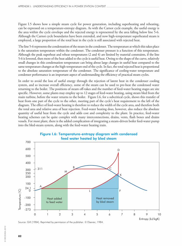
82


Figure I.5 shows how a simple steam cycle for power generation, including superheating and reheating, can be expressed on a temperature-entropy diagram. As with the Carnot cycle example, the useful energy is the area within the cycle envelope and the rejected energy is represented by the area falling below line 5-6. Although the Carnot cycle boundaries have been extended, and now high-temperature superheated steam is employed, a large proportion of the total heat in the cycle is still associated with rejected heat.

The line 5-6 represents the condensation of the steam in the condenser. The temperature at which this takes place is the saturation temperature within the condenser. The condenser pressure is a function of this temperature. Although the peak superheat and reheat temperatures (2 and 4) are limited by material constraints, if the line 5-6 is lowered, then more of the heat added to the cycle is useful heat. Owing to the shape of the curve, relatively small changes in this condensation temperature can bring about large changes in useful heat compared to the same temperature changes at the high-temperature end of the cycle. In fact, the total rejected heat is proportional to the absolute saturation temperature of the condenser. The significance of cooling-water temperature and condenser performance is an important aspect of understanding the efficiency of practical steam cycles.

In order to avoid the loss of useful energy through the rejection of latent heat in the condenser cooling system, and so increase overall efficiency, some of the steam can be used to pre-heat the condensed water returning to the boiler. The positions of steam off-takes and the number of feed-water heating stages are site specific. However, some plants may employ up to 12 stages of feed-water heating, using steam bled from the main turbine, before the water returns to the boiler. Figure I.6, for a subcritical cycle, shows this transfer of heat from one part of the cycle to the other, meeting part of the cycle’s heat requirement to the left of the diagram. The effect of feed-water heating is therefore to reduce the width of the cycle area, and therefore both the total area and relative area of heat rejection. Feed-water heating does, however, also reduce the absolute quantity of useful heat from the cycle and adds cost and complexity to the plant. In practice, feed-water heating schemes can be quite complex with many interconnections, drains, vents, flash boxes and drains vessels. For most plant, there is the added complication of integrating a steam-driven boiler feed-water pump into the bled-steam system, along with the feed-water heating train.

Figure i.6: Temperature-entropy diagram with condensed

feed water heated by bled steam

Heat addedto feed water

Heat removedby bled steam

700

600

500

400

300 311

250200

100

024.1

-100

-200

-273

0 1 2 3 4 5 6 7 8 9 10

Tem

pera

ture

(C

)o

Entropy (kJ/kgK)

D

K

CB

M

FL

A


© O

EC

D/IE

A 2

010

83


Supercritical steam cycles

Higher boiler design pressures raise the boiling temperature and the average temperature of heat addition. If the pressure is raised above water’s critical pressure of 221 bar (saturation temperature 374 °C or 647 K), there is no longer any boiling at constant temperature and operation becomes “supercritical”. The average temperature of heat addition, and therefore steam cycle efficiency, is increased, as in the previous cases where design pressure increased. No separation of water and steam is required, so boilers are designed without a hot reservoir or steam drum. Such boilers are known as “once-through” boilers, with no local recirculation of boiling water around the furnace tube walls. When operating at supercritical pressure, with a steam temperature exceeding 593 °C, the cycle is said to be ultra-supercritical (according to EPRI, although there is no precise definition of this term). An example of a supercritical cycle is shown in Figure I.7, with the pressure line above the critical point and no constant temperature during the heat addition.

Figure i.7: Temperature-entropy diagram of a supercritical steam cycle

590oC

570oC

329oC

270oC

2.9

763

6.3

539

7.1

769

Tem

pera

ture

(C

)o

24.1 Co

700

600

500

400

300

200

100

0

-100

-200

-273

0 1 2 3 4 5 6 7 8 9 10

Entropy (kJ/kgK)


Rankine and Carnot cycle efficiencies

For practical power cycles, efficiency is usually referred to as the Rankine efficiency, which is the useful heat divided by the total heat supplied. This is calculated using the change in the enthalpy of the fluid between key points in the cycle. The equivalent Carnot efficiency can be found by considering the average temperature of heat addition and rejection, which gives the same efficiency as the Rankine calculation. This can also be compared to the hypothetical Carnot efficiency, which is the maximum conceivable efficiency which could have been achieved between the upper and lower temperatures of the cycle. Table I.1 shows a range of cycles: firstly, the basic Rankine cycle, then with the addition of superheat, superheat and reheat, superheat and feed-water heating, reheat and feed-water heating, and finally supercritical operation (with temperatures of 590/570 °C).

© O

EC

D/IE

A 2

010

84


Table i.1: Theoretical rankine efficiency of different cycle configurations

Rankine cycle Efficiency, %

Average temperature ofheat addition

K °C

Basic 41.4 507 234

Superheat 45.8 548 275

Superheat and reheat 47.5 566 293

Superheat and feed-water heating 52.0 619 346

Superheat, reheat and feed-water heating 53.2 634 361

Supercritical pressure 56.5 688 415

source: white (1991).

It can be seen from the table that the power cycle efficiencies are higher than those normally stated for power plant; the differences are due to the effects of real plant losses, including turbine expansion losses (isentropic expansion efficiency), throttling losses, turbine mechanical losses and generator losses. Other differences stem from a range of boiler-related losses, including heat lost in flue gases and radiation losses, and the use of works power. The vapour power cycle parameters therefore provide a foundation for estimating plant performance, but are not the only factors that influence the overall efficiency of power production.

© O

EC

D/IE

A 2

010

85

aPPendix ii: worked examPle of efficiency reconciliation Process

APPeNdix ii: worKed exAMPLe oF eFFiCieNCy reCoNCiLiATioN ProCeSS

This worked example shows how a data submission and simplified calculation scheme of the type proposed

in this report might work in practice.

Assume Plant A has a generating unit “A1” fired primarily with bituminous coal, for which the operator

provides the annual as-run data shown in Table II.1.

Table ii.1: Annual “as-run” data from operator


Total fuel heat used (gross) 17.615 PJ

Total fuel mass consumed 656 713 t

Net electrical power export 1.543 TWh

Net water and steam energy export (where applicable) 2.880 PJ

Fuel energy export (where applicable)* 0.000 PJ

Average CO2 removal efficiency 0.0 %

* some power generation processes supply fuel to other processes (e.g. fuel gas from the gasifier in an igcc plant). this energy

supply must also be accounted for in efficiency calculations.

Although the data provide no detailed breakdown of fuel qualities, the efficiency on a GCV basis can be

calculated directly from the submitted fuel energy and export energy data.

whole plant efficiency = (3.6×1.543+2.880) / 17.615

= 47.9% GCV basis

Efficiency on a net basis is calculated using an NCV estimated from the calculated average fuel GCV and

approximate GCV:NCV ratio from Figure 3.8.

average GCV = 17 615 000 / 656 713 = 26.82 GJ/t

average NCV = 26.82 / 1.0440 = 25.69 GJ/t

whole plant efficiency = (3.6×1.543+2.880) / (17.615/1.0440)

= 50.0% NCV basis

© O

EC

D/IE

A 2

010

86


The power and heat generation efficiencies can then be expressed as:

power generation efficiency = 3.6×1.543 / (17.615 – 2.880)

= 37.7% GCV basis or 39.4% NCV basis

heat generation efficiency = 2.880 / (17.615 – 3.6×1.543)= 23.9% GCV basis or 24.9% NCV basis

Since neither CO2 emissions data nor detailed fuel data are provided, CO2 emissions require estimation. If we assume a C:H ratio of 15.22, since we are told the fuel is primarily bituminous coal, and a GCV for carbon of 32.808 GJ/t and for hydrogen of 141.886 GJ/t then:

energy liberated per tonne of fuel = 26.82 GJ/t = 32.808 C + 141.886 C / 15.22

Where C is the mass fraction of carbon in the fuel. C in this example is therefore 63.66% (ignoring the heating value of the fuel sulphur).

Every tonne of fuel will therefore generate 44/12 × 0.6366 = 2.33 tCO2, which equates to 2.33 / 26.82 = 0.0869 tCO2/GJ on an energy input, GCV basis (or 0.313 tCO2/MWh). From this, the relevant CO2 emission factors can be estimated for power, heat and overall plant output, using the efficiencies calculated above.

CO2 emission per unit of total energy output = 0.0869 / 47.9% = 0.181 tCO2/GJ

CO2 emission per unit of net electrical output = 3.6 × 0.0869 / 37.7% = 0.830 tCO2/MWh

CO2 emission per unit of net heat output = 0.0869 / 23.9% = 0.364 tCO2/GJ

total annual CO2 emissions = 0.0869 × 17 615 000 = 1.53 MtCO2/y

These calculations are summarised in Table II.2

Table ii.2: information that can be derived from the “as-run” data in Table ii.1

Bulk fuel properties

Effective GCV 26.82 GJ/t

Estimated NCV 25.69 GJ/t


Specific emission based on total energy output 0.181 t/GJ

Specific emission based on net electrical output 0.830 t/MWh

Specific emission based on net heat output 0.364 t/GJ

Annual total emissions 1.53 Mt/year

Whole plant overall energy efficiency

GCV basis 47.9 %

NCV basis 50.0 %

Electrical power generation efficiency (net of heat)

GCV basis 37.7 %

NCV basis 39.4 %

If the plant was fitted with CO2 capture equipment, then the above CO2 emission factors would be reduced by the removal efficiency of the capture plant.

Unburned carbon in ash could be deducted from the CO2 emissions calculation, if required, or could be taken into account using standard oxidation factors. However, in reality, such adjustments result in relatively small changes. If unburned loss is required explicitly, then the operator should record this value based on ash sampling.

© O

EC

D/IE

A 2

010

87


The power generation efficiency, calculated on the more conventional basis of power output divided by fuel heat input, would have yielded values of:

power generation efficiency (conventional) = 3.6 × 1.543 / 17.615

= 31.5% GCV basis or 32.9% NCV basis

CO2 emission per unit of net electrical output = 0.0869 × 17 615 000 / 1 543 000 = 0.993 tCO2/MWh

It can be seen that the effect of utilising only a proportion of the waste heat from this plant raises the effective power generation efficiency and reduces the specific CO2 production significantly. In fact, in this example, it could raise efficiency from what would be considered a poor value to what would be considered quite a reasonable value, with a good overall plant fuel energy utilisation level. Although the power exported is not changed by the use of some of the rejected heat, the utilisation of the primary coal energy is significantly improved.

Using the methodology required by the EU CHP Directive yields a 1 percentage point higher power generation efficiency of 38.7% GCV basis for this example because the heat supply is valued more than here (i.e. it is grossed up to an equivalent fuel input value for a stand-alone boiler supplying the same heat).29

It is worth noting that efficiencies of between 31.5% and 50.0% could be quoted for this example plant. This is a good demonstration of why an agreed efficiency reconciliation methodology is needed.

Table ii.3: Supplementary data from operator that can helpdetailed calculation of plant performance


Average running load as % maximum continuous rating (MCR) 62.0 %

Average cooling-water inlet temperature 23.2 °C

Average ambient temperature 18.5 °C

SO2 removal efficiency 90 %

Plant mode of operation Marginal

Fuel 1 Type Bituminous coal

Contribution to total gross heat 89.7 %

Higher heating value 25.70 GJ/t

Average fuel moisture 13.9 %ar

Average fuel ash content 12.70 %ar

Average fuel volatiles content 29.60 %ar

Average fuel sulphur content 1.40 %ar

Fuel 2 Type Heavy oil

Contribution to total gross heat 10.3 %

Higher heating value 43.30 GJ/t

Average fuel moisture 0.2 %ar

Average fuel ash content 0.01 %ar

Average fuel volatiles content 99.20 %ar

Average fuel sulphur content 0.70 %ar

Supporting comments:

29 See footnote 8.

© O

EC

D/IE

A 2

010

88


Where more detailed data are provided, as in Table II.3, more detailed calculations and correlations can be used to determine heating values, CO2 emission factors and other values with more precision.

With this further operating data, it is evident that there is significant oil consumption and that the plant does not generally operate at high load. Both these factors may be due to intermittent or cyclical operation. In practice, some coal-fired plants may also fire natural gas, waste or other opportunity fuels.

Table ii.4: Basic unit data required to calculate correction factors

General plant information Quantity Unit

Plant name Plant A

Country Country C

Location Location L

Plant owner Power Co.

Plant operator O&M Co.

Number of units 2

Unit A1

Commissioning year 1980

Technology type PC (subcritical)

Design fuel type Bituminous coal

Unit rated power generation capacity 450 MWe (gross)

Unit maximum heat supply capacity 160 MWth

Best measured unit overall energy efficiency (GCV, net sent-out basis) 55.0 %

Best measured unit electrical efficiency (GCV, net sent-out basis) 46.0 %

Design fuel GCV 24.0 GJ/t

Design fuel moisture content 10.0 %

Design fuel ash content 12.0 %

Design fuel sulphur content 2.0 %

Cooling-water system type Sea (once-through)

Design main steam temperature 540 °C

Design main steam pressure 160 bar

Number of reheat stages 1

Reheat temperature 540 °C

Flue gas desulphurisation No

Selective catalytic reduction No

Low-NOx burner/over-fire air Yes

Electrostatic precipitator/fabric filtration Fabric filter

Air separation unit No

CO2 capture No

It is now possible to normalise the performance data. The procedure outlined in this report requires some basic data about plant configuration. Such data would be provided on a one-off basis and then used with sets of standard corrections to adjust the reported performance to a known common basis. The general plant data provided are shown in Table II.4.

Heat consumption corrections are needed to bring the plant’s reported performance in line with what would be expected for a plant fitted with FGD, SCR, LNB and OFA, ESP, with a closed-loop wet-tower cooling-

© O

EC

D/IE

A 2

010

89


water system, operating at 80% average load under base-load conditions and with an ambient temperature equivalent to the reference plant. The associated corrections are shown in Table II.5.

Table ii.5: Calculated efficiency correction factors for the “case-study” plant

Correction factor

Particulate control 1.005

Low-NOx burners and over-fire air 1.000

Selective catalytic reduction 0.995

Flue gas desulphurisation 0.980

CO2 capture and storage 1.000

Cooling-water system 0.977

Average running load (part load loss effect) 1.038

Mode of operation 1.010

Ambient temperature 1.009

Case-study plant efficiency correction to normalise 1.013

The performance of a pulverised coal-fired combustion plant is taken as a reference and corrected for the fuel properties and energy supply characteristics of the case-study plant. In the example, a supercritical pulverised coal-fired combustion reference plant with an “as-new” full-load efficiency of 46% on a NCV basis is chosen. The efficiency of this plant under normal operation, mid overhaul cycle, at 80% load factor, with allowance for moderate operational losses and deterioration, is taken to be 42.5% on a GCV basis. The reference case corrections are shown in Table II.6.

Table ii.6: efficiency correction factors for reference plant

Correction factor

Fuel moisture 1.005

Fuel ash 1.000

Fuel sulphur 1.000

Heat export 1.460

Reference plant efficiency correction to normalise 1.467

Steam conditions are not included in the corrections. As discussed in the main report, while it is possible to estimate the impact of different steam conditions on thermal efficiency, it is not appropriate to correct for them here since they are inherent characteristics of a particular plant.

Table II.7 compares the as-run and raw data, and also shows the corrected data for the case-study and reference plants. The potential performance improvements for both CO2 emissions and efficiency can then be determined by comparison.

In the example, it can be seen that, even though the efficiency of the plant is improved significantly through the use of some waste heat, the relative performance is still well below what could be obtained from a modern plant operating under the same conditions.

This example draws attention to the difference between potential for improvement and absolute levels of performance. The use of heat recovery is shown to boost the overall efficiency of a relatively poor plant, and therefore the efficiency of coal utilisation, while the plant still has potential to be much more efficient.

© O

EC

D/IE

A 2

010

90


Table ii.7: overall power plant assessment summary

As-runNormalised

as-runBest practice

Normalised

best practice

Relative

Performance, %


tCO2/GJ total energy output 0.181 0.179 0.207 0.149 20.5

tCO2/MWh net electrical output 0.830 0.819 0.747

tCO2/GJ net heat output 0.364 0.359 n/a

MtCO2/year 1.53

Overall plant efficiency

% GCV basis 47.9 48.5 42.5 59.2 -18.0

% NCV basis 50.0 50.6 44.2 61.6

Power generation efficiency

% GCV basis 37.7 38.2 42.5 51.1 -25.2

% NCV basis 39.4 39.9 44.2 53.1

These calculations are relatively simple to carry out using database software for analysis and comparison. Although accuracy is not high compared to formal test protocols, the method does permit a useful and rapid comparison of performance between plants for the purposes of gauging general levels of performance and identifying outliers.

© O

EC

D/IE

A 2

010

CH-02-701 Efficiency Performance and CO2 Emissions from ...

Documents

Transcript of CH-02-701 Efficiency Performance and CO2 Emissions from ...