CFR Working Paper NO. 16CFR Working Paper NO. 16CFR Working Paper NO. 16CFR Working Paper NO. 16----07070707

Market Power in the Portfolio: Product Market Power in the Portfolio: Product Market Power in the Portfolio: Product Market Power in the Portfolio: Product Market Competition and Mutual Fund Market Competition and Mutual Fund Market Competition and Mutual Fund Market Competition and Mutual Fund

PerformancePerformancePerformancePerformance

SSSS. . . . JaspersenJaspersenJaspersenJaspersen

Market Power in the Portfolio: Product Market Competition

and Mutual Fund Performance

Stefan Jaspersen

This Draft: September 2016

ABSTRACT

I provide evidence that fund managers who overweight firms with the most differentiated

products (‘monopolies’) exhibit a superior risk-adjusted performance. This is consistent with

information advantages due to a better understanding of qualitative information on a firm’s

competitive environment. I find that funds with above median monopoly bets outperform by up

to 92 basis points annually and trade more successfully in both their monopoly and non-

monopoly sub-portfolios. My identification strategy includes exogenous shocks to information

quality using the Sarbanes-Oxley Act and to a firm’s product market environment using the

9/11 terrorist attacks. I document that managers who place larger monopoly bets are less likely

to invest into rival firms at the same time, have a longer investment horizon, and hold more

illiquid and high quality stocks.

JEL classification: G11; G12; G14; G23; L11

Keywords: Mutual fund performance; Information production; Fund manager skill; Investment

behavior; Product market competition

Jaspersen is from the Department of Finance and Centre for Financial Research (CFR), University of Cologne,

Albertus-Magnus-Platz, 50923 Cologne, Germany. E-mail: jaspersen@wiso.uni-koeln.de. The author would

like to thank Alexander Kempf, Monika Gehde-Trapp, Florian Sonnenburg, and seminar participants at the

CFR, University of Cologne, for helpful comments on an earlier draft of the paper.

1

“The key to investing is not assessing how much an industry is going to affect society, or how much it

will grow, but rather determining the competitive advantage of any given company and, above all, the

durability of that advantage. The products or services that have wide, sustainable moats around them

are the ones that deliver rewards to investors.”

- Warren Buffett, Fortune Magazine, November 22, 1999 -

Investors can choose which type of information they acquire and process in their stock selection.

Clearly, information from financial statements is usually easier to collect and evaluate than

softer and qualitative information, such as the firm’s business model, its brand value, or its

competitors. Empirical evidence even suggests that low skill investors underweight information

that is hard to process (e.g., Engelberg, Reed, and Ringgenberg (2012), Hirshleifer, Hsu, and Li

(2013)). However, in the case of venture capitalists, Gompers et al. (2016) document that

qualitative factors are more important for investment decisions than the project’s valuation. In

a similar spirit, Cici et al. (2016) and Gargano, Rossi, and Wermers (2016) argue that more

experienced and sophisticated investors interpret softer information to gain an information

advantage over their peers. Processing qualitative information that leaves more room for

interpretation, hence, seems to offer more valuable trading opportunities for skilled investors

than processing quantitative information. For fund investors, identifying fund managers with

the ability to process qualitative information is highly relevant, as only few actively managed

funds have been shown to outperform (e.g., Barras, Scaillet, and Wermers (2010), Fama and

French (2010)).

In this paper, I use the information on a firm’s competitive environment to differentiate

fund managers by their ability to process qualitative information. Product market competition

is ideal for this purpose. First, it is not obvious for an investor to what extent a firm is threatened

by rivals and how substitutable its product range is. Second, it is not clear whether more or less

competition is desirable for a given firm. Though less competition might increase a firm’s

profitability due to higher price-setting power, it can have a negative impact on corporate

decisions by increasing managerial slack or reducing innovation incentives (e.g., Raith (2003),

2

Hou and Robinson (2006), and Bustamante (2015)). Accordingly, the literature is still

inconclusive on the impact of product market competition on stock market performance. For

example, Aguerrevere (2009) and Gu (2016) find that the relation between competition and

stock returns strongly depends on product market demand and R&D intensity, respectively.

This ambiguity makes the interpretation of a firm’s competitive environment a challenging but

important aspect in investment decisions. Yet, little is known on whether professional investors

exploit this type of information to gain an advantage over their peers.

Anecdotal evidence suggests that a firm’s competition matters for fund managers. Many

seem to follow the Warren Buffett approach and look for firms with a competitive advantage

and few rivals.1 The challenge for these managers is to find firms for which market power

results in a positive stock market outcome. If a fund manager knows about her ability to judge

the consequences of market power for a given firm, she should capitalize on this advantage and

process more product market information when picking stocks. This is in line with theoretical

predictions of Kim and Verrecchia (1994) that some market participants make superior

judgements than others of the same information. In addition, Jiang and Sun (2014) argue that

better information-processing makes informed managers receive a positive signal about a stock

that is unobserved by the remaining investors. As a result, the former place larger bets on the

stock relative to latter. Consequently, larger investments in firms with competitive advantages

signal high attention to and a better understanding of the product market.

Based on this reasoning, I differentiate fund managers by their investment in firms with

competitive advantages and analyze whether this predicts differences in investment skills.

Concretely, I choose the uniqueness of a firm’s products as the source of a competitive

1 E.g., Burton (2012): “Follow the Buffett Strategy” in The Wall Street Journal (August 2, 2012) or Brown

(2012) “Berkshire Follower? Try These 5 Buffett Wannabe Mutual Funds” in Forbes (May 16, 2012). Both

articles point out that managers invest in companies with few competitors to achieve stability in the portfolio

with one fund manager calling these businesses an “ultimate ‘sleep well’ kind of investment” (Burton (2012)).

3

advantage.2 Using mutual fund holdings and the number of rivals for a given firm based on

similarity in 10-K product descriptions (Hoberg and Phillips (2015)), I develop a fund’s

monopoly bet (MB) as the value-weighted fraction of firms with the most differentiated

products, henceforth monopolies, compared to the average portfolio weight of these firms in the

fund’s investment style.

Despite the ambiguous impact on stock returns, investing in monopoly firms is desirable

for several reasons. First, having differentiated products results in more stable cash flows as the

barriers to entry are higher (e.g., Peress (2010), Hoberg, Phillips, and Prabhala (2014)).

Monopoly firms thereby stabilize the portfolio and reduce the manager’s need to frequently

monitor industry dynamics. Holding a larger fraction of monopolies also lowers the risk to

invest into close rivals concurrently, which counteracts undesired correlations and yields a

better diversification over different products. Consistent with this view, recent evidence by

Azar, Schmalz, and Tecu (2016) and Antón et al. (2016) suggests that rival firms are pushed

towards monopolistic behavior if they are concurrently held by the same institutional investor.

On the contrary, fund managers neglecting such connections are therefore at risk for within-

portfolio competition.

Managers might still abstain from investing in monopoly firms. As noted above,

determining the extent of product differentiation and the number of competitors require

information-processing skills. Identifying firms with market power is therefore challenging and

costly, in particular for low-skilled investors. Second, investors try to learn about a company

from similar and related firms (e.g., Foucault and Frésard (2016)). For instance, Alldredge and

Puckett (2016) show that institutional investors exploit economies of scale in information

acquisition and invest in both supplier and customer firms at the same time. The uniqueness of

monopolies, however, hinder information spillovers and learning opportunities. That is why

2 I acknowledge that a firm’s competitiveness not only depends on its product differentiation, but also on market

share, brand value, and price-setting power. Yet, Hoberg and Phillips (2014) argue that firms with more

differentiated products are likely to have a stronger competitive position.

4

fund managers might prefer to invest more aggregately in several close rivals to fully exploit

their research effort.3 Given costs and benefits, it is likely to find cross-sectional differences in

the monopoly bets of fund managers.

My main investigation explores whether larger monopoly bets predict a superior fund

performance. Assuming investors capitalize on their higher information-processing skills of

qualitative information, an overweighting of monopoly firms should indicate a better

understanding of the product market. These managers forgo economies of scale in information

production, but are able to exploit the benefits of monopoly firms. Indeed, two validation

exercises provide first evidence that managers with higher MB put more weight on information

on product market competition. First, they react more strongly to changes in a firm’s number

of rivals. Second, they are more likely to avoid within-portfolio competition. This is consistent

with them targeting the most promising competitor for a product and neglecting rivals firms. In

contrast, managers who ignore these connections or cannot decide among competitors more

likely invest into multiple rivals simultaneously.

Using a broad sample of actively-managed US domestic equity funds in the period from

1999 to 2012, I then find strong support for the main hypothesis that a larger MB positively

predicts performance. Funds with above median MB in a quarter outperform below median MB

funds by up to 92 basis points per year. This result withstands several robustness checks

including different sets of fixed effects or alternative proxies for the propensity to invest in

unique products.

If higher monopoly bets indicate a better understanding of the product market and,

ultimately, higher information-processing skills, then fund managers with these skills should

profit from this information irrespective of the competitive environment of the firm. I therefore

3 In a similar spirit, Hsu et al. (2015) find that analysts exploit the similarity of competing firms and are more

likely to cover a stock if it is a close rival to an already covered firm. Due to lower information production

costs, Engelberg, Ozoguz, and Wang (2013) further show that institutional investors are more likely to hold

firms from the same industry if they are geographically close to each other.

5

examine whether fund managers with larger monopoly bets only select better monopoly stocks

or whether they are also more successful in picking stocks with more competitors. A

performance comparison of buy portfolios indeed provides evidence that funds with larger

monopoly bets trade more successfully in both monopoly- and non-monopoly stocks. This

result also holds when comparing the buy performance with hypothetical buy portfolios

consisting of a firm’s rivals.

To support a causal interpretation for the relationship between the monopoly bet and fund

performance, I exploit two exogenous shocks. First, I use a positive shock to the investors’

information environment with the passage of the Sarbanes-Oxley Act in 2002 (SOX). The

improvement in the quality of public information reduces the advantage of informed investors.

If high-MB funds actually gain information advantages, they should experience a stronger

deterioration in fund performance around the passage of SOX than low-MB funds. My results

from a cross-sectional regression provide support for this assumption with a quarterly

performance decline that is about 1.18 percentage points stronger for funds with above median

MB before SOX. Second, I exploit the 9/11 terrorist attacks as a positive shock to demand and

the number of competitors in the military goods industry. As would be expected from funds

with larger monopoly bets, managers who decrease their position in military good firms around

9/11 exhibit a significantly higher change in fund performance.

In line with differences in information-processing, I provide evidence that the monopoly

bet strongly depends on the manager of the fund, especially on her experience and the effort

she can devote to information acquisition. First, I exploit manager switches of a fund and

document that MB increases around the switch if the new manager has a higher pre-switch

propensity to invest into monopoly stocks than the former manager. Second, I investigate fund

and manager attributes as determinants of the monopoly bet. I hypothesize that MB should be

higher if the manager is more experienced and puts more effort in collecting and processing

information. For one, investment experience should facilitate the processing of qualitative

6

information. Moreover, information-processing is a costly and time-consuming task that

requires effort. Consistently, I find that funds managed by more experienced managers, funds

whose managers do not manage multiple funds concurrently as well as funds managed by

smaller teams with fewer free-riding incentives place larger bets on monopoly firms.

Finally, to further understand why managers with a better understanding of the product

market might choose to overweight monopoly firms and to identify potential channels for the

documented outperformance, I investigate the investment strategies of funds with different MB

levels. Consistent with monopoly stocks providing stability with secure cash flows and less

product market threats, funds with a higher MB have a lower portfolio turnover and hold stocks

over a longer period. Moreover, the lower trading frequency should allow the fund manager to

invest into more illiquid securities to earn a liquidity premium (e.g., Amihud, Mendelson, and

Pedersen (2005)), which is also supported by the results. Finally, their potential profitability

makes monopoly firms suitable instruments to pursue quality investing. In line with this, I show

that funds with higher MB trade more heavily on the Quality-Minus-Junk (QMJ) factor (Asness,

Frazzini, and Pedersen (2014)).

My paper contributes to several strands in the literature. First, the paper relates to the

literature on the information production of investors. Among other things, this literature

classifies the type of information that investors use, e.g., by aggregation level (e.g., Kacperczyk,

Nieuwerburgh, and Veldkamp (2014)), softness and complexity (e.g., Stein (2002), Gargano,

Rossi, and Wermers (2016)), or source (e.g., Coval and Moskowitz (2001), Kacperczyk and

Seru (2007), Fang, Peress, and Zheng (2014)). I contribute to this literature by identifying

product market linkages as hard-to-process information that offers valuable trading

opportunities for investors.

Second, my results contribute to the literature that predicts investment skills from fund

portfolios. Kacperczyk, Sialm, and Zheng (2005), Huang and Kale (2013), and Alldredge and

Puckett (2016) document that funds outperform if they are more concentrated in particular

7

industries or related industries, while Cremers and Petajisto (2009) and Doshi, Elkamhi, and

Simutin (2015) show that more active managers deliver a superior performance. I add to these

studies by differentiating funds by their information-processing skill. Different from the studies

on simultaneous investments in customer and supplier firms, my findings suggest that skilled

investors avoid rival firms from the same industry and rather hold a larger fraction of stocks

from less competitive markets.

Finally, I also contribute to the vast literature on common ownership and the impact of

product market competition on asset pricing (e.g., Hou and Robinson (2006), Hoberg and

Phillips (2010) and Peress (2010)) and corporate behavior (e.g., Giroud and Mueller (2011),

Hoberg, Phillips, and Prabhala (2014), and Azar, Schmalz, and Tecu (2016)). With investment

companies owning around 30% of the US stock market (Investment Company Institute (2015)),

differences in the fund managers’ ability to take product market information into account help

to understand why competition affects stock market performance as well as corporate decisions.

The remainder of the paper is organized as follows. In Section 1, I describe the data and

the monopoly bet measure. Section 2 presents empirical results on the relation of the monopoly

bet fund as well as trade performance and addresses endogeneity concerns. In Section 3, I show

that MB depends on the fund manager. Section 4 examines the relation of MB to the fund’s

investment behavior and identifies potential channels through which the superior performance

emerges, and Section 5 concludes.

1 Data and summary statistics

1.1 Data sources

For my analysis, I combine several data sources. I obtain information on fund characteristics,

e.g., fund returns, total net assets under management, fund fees, fund age, fund families, and

investment objectives from the CRSP Survivor-Bias-Free U.S. Mutual Fund Database (CRSP

8

MF). As the information is at the share-class level, I aggregate it at the fund level by value-

weighting all share class information of a given fund.

I merge CRSP MF with the Thomson Reuters Mutual Fund Holdings Database (MF

Holdings) using the MFLINKS tables. I focus on holdings of common stocks (share codes 10

and 11) and add information about these stocks using the CRSP/Compustat Merged Database.

From the Morningstar Direct Mutual Fund Database (MS Direct) I obtain fund manager

information and come up with a unique identifier for each fund manager. I merge MS Direct

with the former databases using fund cusips.

Finally, I use the Text-based Network Industry Classifications (TNIC) and Product Market

Fluidity Data provided by Hoberg and Phillips (HP) to identify a firm’s product market

competition.4 The HP dataset contains annual pairs of rival firms with a product similarity score

above a certain threshold based on descriptions in 10-K annual filings. The annual number of

pairs per firm therefore identifies the number of close competitors with a higher number

indicating a more competitive product market. I additionally obtain similarity scores and

product market fluidity data from this database. As the pairwise similarity is calculated on an

annual basis, the data allow me to consider dynamics in a firm’s product market competition.

The final sample consists of actively managed diversified U.S. domestic equity funds for

the December 1999 to March 2012 period. To obtain this sample, I first eliminate all

international, sector, balanced, bond, index, and money market funds. Then, I exclude all funds

with less than 50 percent of their assets in common stocks as well as funds with less than ten

stocks, on average. I categorize the remaining funds according to their dominating investment

objective into six style categories using CRSP style codes (Mid Cap (EDCM), Small Cap

4 The data sets can be accessed via http://cwis.usc.edu/projects/industrydata/. An advantage of this classification

is that firms are grouped by the products they offer whereas more traditional classifications (SIC or NAICS)

are based on input factors or production processes. Yet, the data is limited to publicly traded U.S. firms so

competition from private or foreign firms is not taken into account. A detailed description of the data is given,

for example, in Hoberg and Phillips (2015) and Hoberg, Phillips, and Prabhala (2014).

9

(EDCS), Micro Cap (EDCI), Growth (EDYG), Growth & Income (EDYB), and Income

(EDYI)).5 The final sample consists of 2,561 funds managed by 5,002 distinct managers.

1.2 Variable construction and sample characteristics

I sort all stocks in the HP database into quintiles based on the number of product rivals in a

given year. Stocks in the bottom quintile are labeled as monopoly stocks. To obtain a fund’s

monopoly bet each quarter, I calculate the value-weighted fraction of monopoly stocks within

the portfolio using the monopoly information in the current year.6 To rule out that a fund is

placing larger or smaller weights on monopoly stocks due to its stated investment style, I adjust

the fraction of monopoly stocks by subtracting the average monopoly weight within the same

investment style in a given quarter. The monopoly bet (MB), therefore, can be interpreted as an

under- or overweighting of monopoly firms relative to all funds within the same style.7

Panel A of Table 1 reports annual summary statistics for stock characteristics over the

sample period 1999 to 2012. I present information for the whole sample of firms as well as for

monopoly and non-monopoly firms, separately. Panel B of Table 1 reports sample

characteristics for key variables at the fund level. I present information both for the whole

sample of funds as well as for subsamples constructed by stratifying the sample funds into high-

(above median) and low- (below median) MB funds in each period. I use t-tests to test for

differences in means between the subsamples.

– Insert TABLE 1 approximately here –

5 In the rare cases that a share class does not have CRSP Style Code information, I use the old classification

according to Lipper, Strategic Insight, and Wiesenberger to identify a fund’s dominating objective. 6 Note that the portfolio sort is based on all firms in the Hoberg and Phillips data sets while stock holdings of the

mutual funds only contain common stocks. 7 As documented in the robustness section, the main result also holds when using alternative proxies to capture

a fund’s propensity to invest in firms with more unique products.

10

Panel A of Table 1 shows that monopoly firms indeed face fewer product market threats,

as suggested by their lower average product market fluidity. They are significantly smaller and

older than the remaining firms, and have a higher book-to-market ratio. Monopoly firms are

also less liquid, captured by a lower average stock turnover and a higher average Amihud (2002)

illiquidity measure, both constructed using daily data within a quarter. A possible interpretation

of these differences is that the average monopoly firm operates in a specialized niche market

which is more unknown to investors. This is also in line with Hsu et al. (2015) who document

a lower analyst coverage and accuracy for firms in less competitive markets. While monopoly

stocks on average do not have a higher annual return, they are held by more skilled investment

funds, as indicated by their higher Cohen, Coval, and Pástor (2005) stock quality measure using

a fund’s Carhart (1997) 4-factor alpha.8 This is consistent with the view that more skilled fund

managers are better able to identify profitable investment opportunities within the group of

monopoly firms to exploit their benefits.

In terms of fund characteristics, above and below median MB funds differ significantly.

Funds with a higher propensity to overweight monopoly firms are significantly smaller and

slightly younger and come from smaller fund families. They have slightly higher expense ratios,

grow at a higher rate, and hold more stocks in their portfolio. Finally, these funds have an annual

turnover of only 79.20 percent compared to 95.02 percent for below median MB funds. This is

consistent with a higher stability provided by monopoly stocks which reduces the need to

frequently replace stocks. Given that these fund characteristics are known to have an impact on

fund performance, the later performance comparisons will control for these differences. Yet,

even in a univariate comparison larger monopoly bets indicate superior manager abilities as

shown by their significantly higher raw returns, as well as stock characteristic- and risk-adjusted

fund performance. For example, the average quarterly Carhart (1997) 4-factor alpha based on

8 A portfolio approach (not reported), in which I annually sort stocks into quintiles based on the number of

competitors and calculate risk-adjusted performance in the following year, yields a similar picture. A monopoly

stock portfolio does not outperform portfolios of companies with more competitors.

11

gross-of-fee returns in the whole sample amounts to only 23 basis points on an annual basis and

is therefore comparable to other studies. Nevertheless, high-MB outperform low-MB funds by

78 basis points per year.

1.3 Does MB really capture a fund’s response to product market competition?

Table 1 already reveals striking differences in the characteristics of monopoly and non-

monopoly firms. Fund managers might therefore overweight monopolies by chance due to

preferences for other firm characteristics. To validate that the MB measure indeed captures

differences in the reaction to product market information, I analyze the behavior of funds

according to two dimensions: their sensitivity to product market dynamics and their propensity

to invest into rival firms at the same time. Changes in a firm’s competition should induce fund

managers to update their expectations on the future prospects of the firm and to trade on this

new information. This sensitivity should be particularly pronounced for managers with a better

understanding of the product market, as captured by MB.

To measure a fund’s sensitivity, I calculate the R2 from a fund-level regression of changes

in the number of shares held in a stock on lagged changes in the number of rival firms, which

is conceptually similar to the procedure in Kacperczyk and Seru (2007). As the set of rival firms

for a given firm is updated on an annual basis, I calculate annual holdings changes using year-

end reports for each fund and use changes in the number of competitors for all stocks in the

previous two years. I relate Sensitivity of fund i in year t to the fund’s monopoly bet (MB) at the

end of year t-1 and add control variables in the following pooled regression:

, 1 , 1 , 1 ,i t i t i t i tSensitivity MB X (1)

Xi,t-1 is a vector of control variables, which might have an impact on a fund’s sensitivity to

product market dynamics. I control for the logarithm of fund’s total net assets, the logarithm of

12

the fund’s age, the fund’s annual turnover ratio, the fund’s annual total expense ratio, quarterly

fund flows, measured as in Sirri and Tufano (1998), the logarithm of the number of stocks held

by the fund, and the logarithm of the fund family’s total net assets under management. All

independent variables are valid at the beginning of the year, for which I calculate Sensitivity.

To control for unobservable effects in a given period or for a given style, the regressions include

time and style fixed effects. Standard errors are clustered at the fund level.

Panel A of Table 2 reports the results for the regression (1) and for a modified version in

which I replace the MB measure with a dummy that equals one, if the MB of a fund is above the

median in a given period, and zero otherwise (high MB).

– Insert TABLE 2 approximately here –

The results from Panel A of Table 2 support the view that funds with larger monopoly bets

react more strongly to changes in the number of firm rivals. Irrespective of whether I include

additional control variables and fixed effects or not, funds with a higher MB are related to a

higher Sensitivity. The effect is statistically significant at the 1%-level and also economically

relevant with a Sensitivity that is about 0.17 percentage points larger for high-MB funds after

taking fund-level controls and fixed effects into account. Compared to the average Sensitivity

of low-MB funds (2.66 percent) this is equal to a difference of more than 6%.

The second validation exercise is based on the assumption that fund managers overweight

monopoly stocks to avoid within-portfolio competition. If this is the case, we would expect

managers with larger monopoly bets to hold less rival firms at the same time. Consequently,

even in more competitive markets, the manager should only choose a few out of multiple rival

firms.9

9 Alternatively, a manager could hold a long position in one firm while shorting a close competitor (e.g., Akbas,

Boehmer, and Genc (2015)). Due to a lack of data on short-positions in mutual funds, I only present results

based on concurrent long-positions in direct competitors.

13

To test this hypothesis, I calculate for each fund and stock the number of direct competitors

currently held by the fund in the quarter. To avoid a mechanical relation between MB and the

number of competitors held, I limit the analysis to stocks in the non-monopoly sub-portfolio. I

aggregate the number of concurrently held competitors at the fund level by value-weighting

over all stocks in the sub-portfolio. As for the monopoly bet, I use a style-adjusted version of

this measure. I regress the value-weighted number of competitors held on the MB measure or

the MB dummy and the same control variables as in Panel A in the previous quarter as well as

style and time fixed effects. Standard errors are clustered at the fund level. The results are

summarized in the first two columns of Panel B of Table 2. In the last two columns of Panel B,

I repeat the analysis but use the value-weighted number of direct competitors that are

concurrently bought by the fund as dependent variable.10

The results from Panel B of Table 2 show that funds with larger monopoly bets hold and

trade a significantly lower number of direct competitors at the same time, even in their non-

monopoly sub-portfolios. The effect is statistically significant at the 1%-level and also

economically meaningful. Low-MB funds have an average peer-adjusted number of rivals

concurrently held of 0.14 and, thus, on average hold more in close rivals than peer funds. On

the contrary, the peer-adjusted number of close rivals concurrently held is about 0.40 lower for

above median MB funds, as documented in the second column of Panel B. Hence, these funds

on average hold less in close rival firms than peer funds.11

Taken together, the results from this section provide strong evidence that the product

market dimension matters more to funds with larger monopoly bets. This suggests that MB

indeed captures differences in processing this type of information.

10 To obtain the value-weighted number of direct rivals concurrently bought, I calculate for each stock bought by

the fund in a given quarter the number of close rivals that are simultaneously bought. To obtain a fund-level

measure, I aggregate the number of rivals using the trade size as a weight. 11 In Table A.1 in the Internet Appendix, I provide further evidence that high-MB funds more actively avoid

within-portfolio competition by documenting that they are more likely to replace rival firms, i.e., they have a

stronger tendency to sell a stock with a higher similarity to the stocks that newly enter the portfolio during the

quarter.

14

2 Monopoly bets and future fund performance

In this section I examine the hypothesis that funds with a better understanding of the product

market place larger monopoly bets and gain an information advantage leading to a higher fund

performance. I formally test this hypothesis in Section 2.1. In Section 2.2, I analyze differences

in buy performance in monopoly and non-monopoly stocks. Then, in Section 2.3, I investigate

whether the result on the MB-performance relation is robust to variations in the empirical setup.

In Section 2.4, I address endogeneity concerns for the MB-performance relationship by

exploiting exogenous shocks to the information environment and to a firm’s product market

competition.

2.1 Do monopoly bets predict fund performance?

To examine the relation between a fund’s performance and its monopoly bet, I employ both

holdings-based performance measures as well as standard factor models to estimate fund

performance. In particular, throughout the paper, I present results based on the stock-

characteristic-adjusted performance measure of Daniel et al. (1997) (DGTW) and based on a

Carhart (1997) 4-factor model.12 I compound the monthly DGTW-adjusted fund returns over

the three months within a quarter. Quarterly alphas from the factor model are constructed as the

difference of the realized excess fund return and the expected excess fund return in the quarter.

The expected return in a given month is calculated using factor loadings estimated over the

previous 24 months and factor returns in the current month. I compound both realized and

expected excess returns over the three months of a quarter before taking their difference.13 To

better capture the investment skill of the fund manager, I use gross-of-fee returns, i.e., the net-

of-fee return plus one twelfth of the annual total expense ratio, to calculate alphas.

12 For robustness, I ran the analysis also based on different holdings-based performance measures as well as

different factor models. As shown in the robustness section, my main result does not change when using these

alternative performance measures. 13 Monthly factors are obtained from Kenneth French’s website. Monthly alphas and factor loadings are only

calculated, if none of the returns in the past 24 months are missing. Therefore, younger funds are excluded

from the analysis which helps alleviate the concern of an incubation bias (Evans (2010)).

15

The univariate comparisons in Panel B of Table 1 already hint at a superior performance

of funds with above median MB. In a more formal test, I now employ a pooled regression in

which I relate fund performance in quarter t to its monopoly bet, MB, in quarter t-1 and add

control variables that are known to have an impact on fund performance:

, 1 , 1 , 1 ,i t i t i t i tPerf MB X (2)

I measure fund performance (Perf) as described above. Xi,t-1 is a vector consisting of the

control variables as in Table 2 except for the expense ratio. All independent variables are lagged

by one quarter. As before, I run regressions with style and time fixed effects and cluster standard

errors at the fund level. Table 3 reports the results for regression (2) both using the continuous

MB variable as well as the high-MB dummy.

– Insert TABLE 3 approximately here –

The results in Table 3 support the hypothesis for a positive relation between MB and fund

performance. For both, the continuous MB measure and the MB dummy, I find that larger

monopoly bets are positively related to fund performance. The effect is also economically

relevant: After controlling for various fund characteristics, funds with above median MB

outperform funds with below median MB by around 23 basis points per quarter when using

DGTW-adjusted returns or by around 18 basis points per quarter using Carhart (1997) 4-factor

alphas. This corresponds to an annual outperformance of up to 92 basis points.

Regarding the coefficients on the control variables, I find that fund size has a negative

impact on fund performance suggesting diseconomies of scale in the mutual fund industry (Berk

and Green (2004)). While fund age has a positive impact on fund performance, turnover is

negatively related to performance, the latter being consistent with Carhart (1997) or Barras,

Scaillet, and Wermers (2010)). Finally, I find a positive impact of family size on fund

performance, in line with Chen et al. (2004) and Pollet and Wilson (2008). However, the

16

relation is statistically insignificant which is consistent with more recent evidence by Bhojraj,

Cho, and Yehuda (2012). The remaining controls have no consistent impact on performance.

In sum, the results from this section support the notion that funds with a better

understanding of the product market, as captured by a higher MB, obtain an information

advantage which is beneficial for their performance.

2.2 Evidence from trades in monopoly and non-monopoly stocks

If monopoly bets signal an information-processing skill, then this skill should be reflected

irrespective of a firm’s competitive environment. In this section, I therefore explore whether

the better comprehension of product market competition of managers with higher monopoly

bets also allows them to outperform in more competitive markets. For one, Peress (2010) shows

that more competitive markets are less informationally efficient. Skilled fund managers should

exploit the inefficiencies in these segments to generate a higher performance than their unskilled

peers.14 Second, a higher fraction of monopoly stocks reduces the need to constantly monitor

industry dynamics, so fund managers can devote more attention to firms with stronger

competition. I therefore explore the performance of trades in monopoly and non-monopoly sub-

portfolios.15 For each fund, I identify a buy decision if the number of shares held by the fund at

the end of a quarter has increased compared to the previous quarter. I calculate the buy

performance of the sub-portfolios as the trade size-weighted performance of all the stocks in

the sub-portfolio in the following quarter using DGTW-adjusted returns and Carhart (1997) 4-

factor alphas. Risk-adjusted quarterly stock performance is calculated analogously to fund

14 A similar argument is made by Fang, Kempf, and Trapp (2014) who document that a manager’s skill is

rewarded more in the less efficient high yield bond market segment. 15 Several studies argue that trades are more appropriate than holdings to capture information advantages, and,

hence, skill of fund managers (e.g., Chen, Jegadeesh, and Wermers (2000), Pool, Stoffman, and Yonker

(2015)).

17

performance. I run a similar regression as in Table 3, but replace the dependent variable with

the performance of the buy sub-portfolios. Panel A of Table 4 reports the results.

– Insert TABLE 4 approximately here –

Table 4 results provide clear evidence for an information advantage of high-MB funds

irrespective of the competitive environment. For both monopoly- and non-monopoly stocks, the

buy portfolios of funds with higher MB outperform the buys of funds with lower MB. For

example, the monopoly buys of high-MB funds outperform by almost 21 basis points per quarter

when using Carhart (1997) alphas.

To provide further support for the higher stock-picking skills of funds with larger monopoly

bets, I compare their actual buy performance with the performance of hypothetical benchmark

sub-portfolios consisting of the competing firms of the purchased stocks. To obtain the

benchmark, for each stock, I calculate the equally-weighted average quarterly performance of

its rivals firms using TNIC data. For each fund, I then calculate the trade-size weighted average

performance of the rivals in the buy portfolios. This can be interpreted as the performance of a

fund’s buy portfolio if the amount that was actually used to purchase a stock had been equally

distributed over the stock’s rival firms. I calculate the differences between the actual buy sub-

portfolio and the benchmark portfolios and use this difference as dependent variable in an

analogous regression as in Panel A. Panel B of Table 4 reports the results.

The results from Panel B of Table 4 additionally support the notion that fund managers

with larger MB are more successful in identifying the most promising firms out of close rival

firms as their actual buy portfolios outperform the rival firms’ performance to a larger extent.

In Table A.2 of the Internet Appendix, I also present evidence from a long-short strategy

as an alternative approach to document information advantages in monopoly and non-monopoly

sub-portfolios. In detail, the results in Panel A of Table A.2 suggest that buying stocks bought

by high-MB funds and selling the stocks sold by these funds delivers a significantly higher

18

performance than a long-short strategy based on the trades of low-MB funds. This result is

robust to the inclusion of time fixed effects as well as standard errors clustered at the fund level,

as summarized in Panel B of Table A.2.

Taken together, the main result of Table 3 is supported by these trade-based results. More

importantly, the outperformance of high-MB funds does not stem from a specialization in

monopoly firms, but also from their trading in more competitive product markets. This is

consistent with the idea that funds with a better comprehension of the product market are able

to exploit investment opportunities irrespective of a firm’s competitive position.

2.3 Robustness and alternative specifications

In this section, I present results from a battery of robustness tests for the main result of Table 3.

Panel A of Table 5 reports results when using different performance measures, both based on

factor models as well as holdings-based measures, as dependent variable. For brevity, here and

in the rest of the Table 5, I suppress control variables. As alternative factor models, I estimate

quarterly fund performance using a Jensen (1968) 1-factor, a Fama and French (1993) 3-factor,

a Pástor and Stambaugh (2003) 5-factor as well as Cremers, Petajisto, and Zitzewitz (2012) 4-

factor and 7-factor models. Finally, I calculate a fund’s value-weighted average Cohen, Coval,

and Pástor (2005) stock quality measure which is the Carhart (1997) 4-factor alpha, estimated

over the last 24 months, of all funds holding a stock in a particular period.

In Panel B of Table 5, I vary the estimation method. In particular, I estimate the regression

(2) using fund fixed effects, manager fixed effects, family-time fixed effects or style-time fixed

effects to control for any unobservable effects at the fund or manager level or within a given

family or investment style in a quarter.16 Next, I perform a permutation test in which I assign a

16 The fund family, for example, could employ more analysts to facilitate the processing of qualitative

information. Alternatively, monopoly firms could be geographically close to certain fund families that

overweight these stocks due to a (profitable) local bias (Coval and Moskowitz (2001)).

19

fund a random MB (high-MB dummy) and rerun my baseline regression of Table 3. This is

repeated for 10,000 random draws. The p-value of this exercise indicates the number of draws

that result in a regression coefficient as large as or larger than the reported coefficient of Table

3. To take into account that high-MB and low-MB funds differ significantly on observable

characteristics, I finally run the baseline regression on a weighted sample where weights are

based on a propensity score matching. To estimate propensity scores, I estimate a logistic

regression of the high-MB dummy on all control variables of regression (2) as well as time and

style fixed effects. This approach overweights observations from low-MB funds that are more

similar to the high-MB group based on observable fund characteristics.

As a last set of robustness tests, Panel C of Table 5 reports results when I use alternative

approaches to measure a fund manager’s propensity to invest in firms with fewer competitors

as a signal for understanding product market competition. These include the equally-weighted

instead of the value-weighted fraction of monopoly stocks, the value-weighted number of close

rivals over all stocks in the fund portfolio, the definition of monopoly firms based on low

product market fluidity as well as the value-weighted product market fluidity of all firms in the

fund portfolio.17

– Insert TABLE 5 approximately here –

All tests in Table 5 support the result that funds with a stronger propensity to invest into

monopolies deliver a superior performance. In particular, the result is statistically significant in

all specifications and economically similar to the one in Table 3. I can therefore conclude that

my main result is robust to variations in the empirical setup.

17 Note that in the last approach, a higher product market fluidity indicates stronger product market threats.

Therefore a higher value indicates a lower tendency to invest into monopoly stocks. In unreported tests, I also

used the value-weighted number of rivals concurrently held or traded, as in Panel B of Table 2, to proxy a

better understanding of the product market. As expected, the results show that these measures have a

significantly negative impact on fund performance.

20

2.4 Exogenous shocks to information quality and competitive environment

In this section, I exploit two quasi-natural experiments to support a causal interpretation of the

previously established performance result. In Section 2.4.1, I use the Sarbanes-Oxley Act in

2002 as an exogenous shock to the overall quality of publicly-available information and in

Section 2.4.2, I provide results from an exogenous shock to the competitive environment in the

military goods industry after the 9/11 terrorist attacks.

2.4.1 Evidence from a shock to information quality around the Sarbanes-Oxley Act

If fund managers with larger monopoly bets obtain an information advantage by incorporating

hard-to-process information, then this advantage should be diminished, once the overall

reporting quality of firm information improves. With the passage of the Sarbanes-Oxley Act

(SOX) in 2002 firms face enhanced requirements in their financial reporting which generally

improves the information set of investors. This makes it less likely for informed investors to

fully reap the profits from their privately obtained information (e.g., Bernile, Kumar, and

Sulaeman (2015)). I therefore expect a stronger deterioration in fund performance around SOX

for funds with larger monopoly bets before the event. To test this hypothesis, I run a cross-

sectional regression similar to Agarwal et al. (2015) of the change in fund performance,

measured as the difference between average quarterly performance in the four quarters after the

event and the four quarters before the event on the average quarterly MB in the four quarters

before SOX and the same control variables as in equation (2), all averaged over the same

quarters as MB except for fund age, which is measured at the event quarter. The regression also

includes style fixed effects. Table 6 reports the results from this exercise using both the

continuous average MB measure as well as a dummy variable equal to one, if the fund has an

average MB above the median, and zero otherwise.

– Insert TABLE 6 approximately here –

21

The results in Table 6 provide support for the hypothesis that funds with larger monopoly

bets experience a stronger decline in fund performance around the passage of SOX. For

example, funds with above median average MB before the event quarter experience a decline

in quarterly performance of 1.18 percentage points in terms of DGTW-adjusted returns relative

to below median average MB funds.18

These results suggest that the improvement in the quality of publicly available information

induced by the passage of the Sarbanes-Oxley Act in 2002 hurts the more informed investors

to a larger extent. This is consistent with the notion that high-MB funds indeed have an

information advantage over low-MB funds.

2.4.2 Evidence from a large shock to competition around the 9/11 terrorist attacks

As an additional identification strategy I use an exogenous shock to the military goods industry

due to the 9/11 terrorist attacks. The positive demand shock in the defense industry after the

attacks led to increases in competition as new firms entered the industry or existing firms

changed their product offerings towards the higher demand. This resulted in higher product

similarity and more direct rivals for military good firms (Hoberg and Phillips (2015)).

Consequently, fund managers who place larger monopoly bets should reduce their position in

military good firms after the sudden increase in competition. Therefore, I expect funds with

decreases in the portfolio weight of military goods firms to exhibit a higher performance change

around the event.

18 To rule out the concern of a potential mean reversion in fund performance, I repeat the analysis using Q4/2005

as a placebo period without a similar regulatory shock. The results, reported in Panel A of Table A.3 in the

Internet Appendix, suggest that, in the absence of an information shock, funds with higher MB do not

experience a significant decline in fund performance. The comparison of the coefficients for the SOX quarter

and the placebo period, summarized in Panel B of Table A.3, shows that the decline in performance around

SOX is significantly larger than in the placebo period.

22

To implement this idea, I identify competitors that operate in the military goods industry

in the year 2000 prior to the attack using the HP data.19 For each fund with a positive weight in

the military industry before the attack I calculate post-minus-pre-attack average weights in these

military firms using quarterly values in the four quarters before the terrorist attacks, i.e., from

September 2000 to June 2001, and after the attacks in the period March to December 2002. I

skip the quarter directly after the terrorist attacks as the industry change is likely to develop

over a couple of months. Similar to the MB measure, I use peer-group adjusted average weights

before and after the attack to control for style driven differences in the exposure to military

firms.20 For the same period, I calculate post-minus-pre-attack differences in average quarterly

fund performance. Table 7 reports results from a cross-sectional regression in which I relate the

performance difference to the military weight difference and control for the same variables as

before using average values in the four quarters before the attack as well as style fixed effects.

I present results both for the continuous difference in military weights as well as for a modified

version in which I replace the difference with a dummy that equals one, if the fund’s change in

its military weight is above the median of all funds.

– Insert TABLE 7 approximately here –

As expected, the results from Table 7 suggest a negative relation between performance

changes and changes in the weight of military goods firms. For instance, funds with above

median changes in their peer-adjusted weight in military good firms after the attack show a

decrease in average quarterly Carhart (1997) 4-factor alpha by almost 47 basis points compared

to funds with below median changes. This is a significant effect and unlikely to stem solely

from trading in the military goods industry but from trading in the whole portfolio. I argue that

19 I take General Dynamics as focal firm in the military industry and identify all its close rivals. For these rival

firms, I search for additional competitors that are not already identified as a rival to General Dynamics. I repeat

this step once again for the additional competitors to identify a broader range of firms operating in the military

goods industry. 20 The results (unreported) remain qualitatively unchanged when using unadjusted weights in military good firms.

23

managers who decrease their military weight are generally better in incorporating product

market shocks and therefore adjust their total portfolio according to this new information.

These results provide evidence that a positive shock to the product market competition

within an industry and a subsequent reduction in the industry weight, as would be expected for

funds with higher monopoly bets, bring about changes in fund performance. This strengthens a

causal interpretation of the relation between fund performance and a fund’s investment into

more differentiated products.

3 Is MB capturing a manager-related characteristic?

In this section, I provide evidence that the monopoly bet results from differences in information-

processing by showing that it is related to the fund manager and her characteristics. If MB

depends on the fund manager, we should see changes in a fund’s monopoly bet when the

manager is replaced. I therefore identify cases when a single-managed fund is taken over by

another single manager and calculate changes in average quarterly monopoly bets in the year

before and after the switch quarter.21 I compare the new manager’s propensity to invest into

monopoly stocks, measured as the average monopoly bet of the new manager in the year before

the switch over all of her (team- and single-managed) funds, with the average monopoly bet of

the old manager in the respective fund (∆ MB propensity). If the new manager tends to place

larger monopoly bets than the old manager, then the fund’s monopoly bet should increase

around the switch.

Panel A of Table 8 provides results of a pooled regression in which I regress the fund’s

change in MB around the manager switch on the difference in fund managers’ monopoly bet

propensities. I control for the same variables as in Table 2, measured at the end of the switch

21 Jin and Scherbina (2011) provide evidence that newly appointed managers only need two quarters to implement

their own investment strategy in the fund portfolio.

24

quarter, as well as style and time fixed effects. Standard errors are, as before, clustered at the

fund level.

– Insert TABLE 8 approximately here –

The results in Panel A of Table 8 support the hypothesis that a new manager with a stronger

propensity to invest into monopoly firms than the old manager increases the fund’s MB.22

After having documented a general influence of the fund manager on the propensity to

invest into monopoly firms, an obvious question that arises is if different manager attributes

predict differences in MB. The robustness tests in Panel B of Table 5 already rule out that the

relation between MB and performance is driven by time-invariant skill differences between

management teams. It is, thus, unlikely that the ability to process qualitative information stems

only from the manager’s innate talent. However, it is possible that fund managers learn to

process qualitative information and to better understand the product market. Moreover, their

job should allow them to put sufficient effort in costly information acquisition.

I conjecture that the monopoly bet depends on manager experience as well as the effort she

devotes to manage the fund. To capture manager effort, I introduce a dummy variable equal to

one if the fund’s managers on average manage more than one fund (Multiple funds per

manager), and zero otherwise. Agarwal, Ma, and Mullally (2016) find that managers divert

their effort when managing multiple funds. If larger monopoly bets require more effort in

information production, then managers with multiple funds are less likely to overweight

monopoly stocks.

In addition, more experienced fund managers should be better in processing information

on a firm’s product market due to its qualitative nature. Therefore, I predict the manager’s

investment experience to be positively related to the fund’s monopoly bet. As a proxy for

22 This results also holds when controlling for fund performance, measured as the Carhart (1997) 4-factor alpha

over the past 24 months.

25

investment experience, I use the maximum number of years working in the fund industry over

all managers of the fund (Manager tenure).23

Lastly, I use the number of fund managers as additional determinant (# Managers). Larger

teams can produce more information at the same time when each member is allocated a subset

of stocks to evaluate. The resultant higher attention on each firm should facilitate the

incorporation of product market information into the stock selection. However, larger groups

induce managers to free-ride on the effort of others and to engage less in information production

(e.g., Patel and Sarkissian (2015)). Moreover, soft information leaves more room for

disagreement among team members, suggesting that larger teams prefer to focus on hard

information (Stein (2002)). It is therefore an empirical question whether larger fund manager

teams place larger monopoly bets.

To test these hypotheses, I run pooled OLS regressions in which I relate MB to the

mentioned manager attributes in the previous quarter also taking into account the same control

variables as in Panel A, as well as time and style fixed effects. Again, standard errors are

clustered at the fund level. I conduct a similar analysis using the MB dummy as dependent

variable in a logistic regression. Panel B of Table 8 presents the results of this analysis.

Based on the results presented in Panel B of Table 8, I find support for the notion that time-

varying manager characteristics matter for the propensity to invest into monopoly stocks. As

hypothesized, managers who can devote more effort in information production as well as

managers with more investment experience place larger monopoly bets. On the other hand,

funds managed by larger teams invest less in monopoly stocks, which is consistent with free-

riding in information production.

Taken together, results from this section provide strong evidence for a manager-related

explanation of why funds differ in their monopoly bet and why these differences predict fund

23 Manager tenure is measures as the difference in years between the current month and the manager’s first

appearance as US domestic equity fund manager in the Morningstar Direct database.

26

performance. This is consistent with information on product market competition requiring effort

and experience in information production and processing.

4 MB and fund investment behavior

To further understand the manager’s motivation to invest into monopoly firms when

incorporating information on the competitive environment and to identify potential channels for

the documented outperformance, I finally analyze whether monopoly bets are employed by fund

managers to pursue particular investment strategies.

Higher monopoly bets could be the result of long-term trading strategies as monopoly firms

generate more stable cash flows. If this is the case, investors should hold on to monopoly stocks

for a longer period of time. On the contrary, firms with less market power more often adapt

their strategies due to a dynamic competitive environment, e.g. by investing more in R&D or

increasing acquisition activity. This leads to a more frequent updating of investors’ expectations

about the firm’s future cash flows (see, e.g., Giannetti and Yu (2016) and Irvine and Pontiff

(2009)). Hence, stocks from competitive industries seem to be more appropriate for short-term

investors.

To test, whether funds with larger monopoly bets are indeed more long-term oriented, I

estimate pooled regressions where the dependent variable is the fund’s trading frequency in

quarter t. I use both the fund’s quarterly turnover of the common stock portfolio (Portfolio

turnover) and the “Simple Horizon Measure” of Lan, Moneta, and Wermers (2016), measured

as the value-weighted average number of years that the currently held stocks are kept in the

portfolio (Investment horizon), as proxies for trading frequency. I annualize Portfolio turnover

by multiplying it with four. The key independent variable is MB or the MB dummy in quarter

t-1. I control for the same control variables as in Table 2 and include time and style fixed effects

while standard errors are clustered at the fund level. Regression results are summarized in Panel

A of Table 9.

27

– Insert TABLE 9 approximately here –

Results from Panel A of Table 9 support the hypothesis that managers with higher

monopoly bets keep the stocks for a longer period of time, irrespective of whether I use

Portfolio turnover or Investment horizon. The effect is significant both in statistical (significant

at the 1%-level) and economic terms. For example, the portfolio turnover of high-MB funds is

almost eight percentage points per year lower than the turnover of low-MB funds. In addition,

the Investment horizon is about 0.21 years longer for funds with above median MB. Compared

to the average Investment horizon of low-MB funds (3.76 years) this is a difference of about six

percent.24

In Table A.4 in the Internet Appendix, I additionally present results when calculating

Investment horizon separately for monopoly- and non-monopoly sub-portfolios. The results

provide strong evidence that funds with larger monopoly bets hold both monopoly and non-

monopoly stocks for a longer time, while the difference is more pronounced in the monopoly

sub-portfolios. This is not surprising considering that high-MB funds pick better performing

monopoly stocks, as shown in Table 4, and have less incentives to sell monopoly stocks than

low-MB funds.

The stability and resultant lower trading frequency should further allow the fund manager

to pursue riskier strategies and invest more costly, e.g., in more illiquid assets to earn an

illiquidity premium (see, e.g., Amihud, Mendelson, and Pedersen (2005)). I test this hypothesis

by calculating the fund’s portfolio liquidity following Massa and Phalippou (2005) as the value-

weighted average stock liquidity measure (Portfolio liquidity). I run a similar regression as in

Panel A of Table 9 using Portfolio liquidity as dependent variable. Columns 1 and 2 of Panel B

24 This result, admittedly, raises the concern that the monopoly bet is just an alternative proxy for the fund’s

holding horizon. Since Lan, Moneta, and Wermers (2016) document that long-horizon funds outperform, the

previously established outperformance of high-MB funds could therefore simply stem from a longer investment

horizon. However, in unreported tests, I add the fund’s investment horizon as control variable in the regression

of Table 3 and still find a significant and positive impact of MB on fund performance.

28

in Table 9 present the results. As expected, funds with larger monopoly bets have a significantly

(at the 1%-level) lower portfolio liquidity. The difference is almost 0.42 between high- and low-

MB funds which represents about 5.8 percent of the Portfolio liquidity of low-MB funds (7.19).

Finally, monopoly stocks might also be used as instruments for mispricing-related trading.

As market power could result in safety, growth, and profitability of the firms, monopoly stocks

are likely candidates for high quality stocks (Asness, Frazzini, and Pedersen (2014)). I therefore

estimate a fund’s quarterly loading on the “Quality-Minus-Junk” (QMJ) factor from a Carhart

(1997) 4-factor model augmented by the QMJ factor and the “Betting-Against-Beta” (BAB)

factor (Frazzini and Pedersen (2014)) using daily gross fund returns within the quarter (Fund

QMJ loading).25 The results of the same pooled regression as before, but with Fund QMJ

loading as dependent variable, are presented in columns 3 and 4 of Panel B. These results

provide support for the notion that funds with larger monopoly bets pursue more quality

investing. Compared to the Fund QMJ loading of below median MB funds (-0.13) the loading

of high-MB funds is by about one-third larger.26

In sum, the results from this section suggest that the monopoly character of stocks is

exploited for concrete investment strategies. Especially, a higher fraction of monopoly stocks

is indicative for profitable trading behavior, such as investments in illiquid stocks and quality

investing, which should contribute to the outperformance of high-MB funds.

5 Summary and conclusion

Despite the importance of product market competition for asset pricing and corporate decisions,

surprisingly little is known about the impact of firm competition on the performance and

behavior of professional investors. Only recently, academic research suggests that institutional

investors try to avoid rivalry among their portfolio firms and rather push them towards

25 I obtain daily BAB and QMJ factors from AQR’s website: https://www.aqr.com/library/data-sets. 26 In unreported tests, I replace Fund QMJ loading with the loading on the operating profitability factor (RMW)

from a Fama and French (2015) 5-factor model. The results remain qualitatively unchanged.

29

monopolistic behavior (e.g., Azar, Schmalz, and Tecu (2016)). In this paper I study how the

incorporation of the product market dimension into stock picking decisions affects the

performance of fund managers. A firm’s product market environment is more challenging to

capture than quantitative information and, thereby, offers valuable information for investors

with higher information-processing skills.

I develop the monopoly bet as a simple measure to differentiate managers by their ability

to process information on a firm’s competitive environment and document that mutual fund

managers who place larger bets on firms with the most differentiated products gain information

advantages and exhibit a superior performance. Furthermore, my tests based on an exogenous

shock to the quality of public information as well as an exogenous demand shock in the military

goods industry suggest a causal interpretation of the link between a fund’s propensity to

overweight monopoly firms and its performance.

Consistent with differences in information-processing ability, I further provide evidence

that the tendency to invest into monopoly firms is likely a time-varying manager attribute and

strongly depends on her investment experience and effort.

As expected, managers with larger monopoly bets avoid concurrent investment in close

rivals and hold stocks for a longer period. Finally, they exploit the monopoly character of the

firms to pursue more illiquid and quality investment strategies which are documented to

positively affect performance.

Taken altogether, it appears that skilled professional investors can extract valuable

information from a firm’s product market environment and exploit this hard-to-process

information to gain an advantage over their peers.

30

REFERENCES

Agarwal, V., L. Ma, and K. Mullally. 2016. Managerial Multitasking in the Mutual Fund

Industry. Working Paper, Georgia State University and Northeastern University.

Agarwal, V., K. A. Mullally, Y. Tang, and B. Yang. 2015. Mandatory Portfolio Disclosure,

Stock Liquidity, and Mutual Fund Performance. Journal of Finance 70: 2733-76.

Aguerrevere, F. L. 2009. Real Options, Product Market Competition, and Asset Returns.

Journal of Finance 64: 957-83.

Akbas, F., E. Boehmer, and E. Genc. 2015. Peer Stock Short Interest and Future Returns.

Working Paper, University of Kansas, Singapore Management University, and Erasmus

University Rotterdam.

Alldredge, D. M., and A. Puckett. 2016. The Performance of Institutional Investor Trades

Across the Supply Chain. Working Paper, Washington State University and University

of Tennessee, Knoxville.

Amihud, Y. 2002. Illiquidity and Stock Returns: Cross-Section and Time-Series Effects.

Journal of Financial Markets 5: 31-56.

Amihud, Y., H. Mendelson, and L. H. Pedersen. 2005. Liquidity and Asset Pricing. Foundations

and Trends in Finance 1: 269-364.

Antón, M., F. Ederer, M. Giné, and M. Schmalz. 2016. Common Ownership, Competition, and

Top Management Incentives. Working Paper, IESE Business School, Yale University,

and University of Michigan.

Asness, C. S., A. Frazzini, and L. H. Pedersen. 2014. Quality Minus Junk. Working Paper, AQR

Capital Management, Copenhagen Business School, and New York University.

Azar, J., M. C. Schmalz, and I. Tecu. 2016. Anti-Competitive Effects of Common Ownership.

Working Paper, University of Navarra, University of Michigan, and Charles River

Associates.

Barras, L., O. Scaillet, and R. Wermers. 2010. False Discoveries in Mutual Fund Performance:

Measuring Luck in Estimate Alphas. Journal of Finance 65: 179-216.

Berk, J. B., and R. C. Green. 2004. Mutual Fund Flows and Performance in Rational Markets.

Journal of Political Economy 112: 1269-95.

Bernile, G., A. Kumar, and J. Sulaeman. 2015. Home away from Home: Geography of

Information and Local Investors. Review of Financial Studies 28: 2009-49.

Bhojraj, S., Y. J. Cho, and N. Yehuda. 2012. Mutual Fund Family Size and Mutual Fund

Performance: The Role of Regulatory Changes. Journal of Accounting Research 50:

647-84.

Forbes, May 16, 2012. 2012. Berkshire Follower? Try These 5 Buffett Wannabe Mutual Funds.

May 16, 2012.

The Wall Street Journal, August 2, 2012. 2012. Follow the Buffett Strategy. August 2, 2012.

Bustamante, M. C. 2015. Strategic Investment and Industry Risk Dynamics. Review of

Financial Studies 28: 297-341.

Carhart, M. M. 1997. On Persistence in Mutual Fund Performance. Journal of Finance 52: 57-

82.

Chen, H.-L., N. Jegadeesh, and R. Wermers. 2000. The Value of Active Mutual Fund

Management: An Examination of the Stockholdings and Trades of Fund Managers.

Journal of Financial and Quantitative Analysis 25: 343-68.

Chen, J., H. Hong, M. Huang, and J. D. Kubik. 2004. Does Fund Size Erode Mutual Fund

Performance? The Role of Liquidity and Organization. American Economic Review 94:

1276-302.

Cici, G., M. Gehde-Trapp, M.-A. Goericke, and A. Kempf. 2016. What They Did in Their

Previous Lives: The Investment Value of Mutual Fund Managers’ Experience Outside

31

the Financial Sector. Working Paper, Centre for Financial Research, University of

Cologne.

Cohen, R. B., J. D. Coval, and L. Pástor. 2005. Judging Fund Managers by the Company They

Keep. Journal of Finance 60: 1057-96.

Coval, J. D., and T. J. Moskowitz. 2001. The Geography of Investment: Informed Trading and

Asset Prices. Journal of Political Economy 109: 811-41.

Cremers, K. J. M., and A. Petajisto. 2009. How Active Is Your Fund Manager? A New Measure

That Predicts Performance. Review of Financial Studies 22: 3329-65.

Cremers, M., A. Petajisto, and E. Zitzewitz. 2012. Should Benchmark Indices Have Alpha?

Revisiting Performance Evaluation. Critical Finance Review 2: 1-48.

Daniel, K., M. Grinblatt, S. Titman, and R. Wermers. 1997. Measuring Mutual Fund

Performance with Characteristic-Based Benchmarks. Journal of Finance 52: 1035-58.

Doshi, H., R. Elkamhi, and M. Simutin. 2015. Managerial Activeness and Mutual Fund

Performance. Review of Asset Pricing Studies 5: 156-84.

Engelberg, J., A. Ozoguz, and S. Wang. 2013. Know Thy Neighbor: Industry Clusters,

Information Spillovers and Market Efficiency. Working Paper, University of California,

San Diego, Rice University, and University of North Carolina.

Engelberg, J. E., A. V. Reed, and M. C. Ringgenberg. 2012. How are Shorts Informed?: Short

Sellers, News, and Information Processing. Journal of Financial Economics 105: 260-

78.

Evans, R. B. 2010. Mutual fund incubation. Journal of Finance 65: 1581-611.

Fama, E. F., and K. R. French. 1993. Common Risk Factors in the Returns on Stocks and Bonds.

Journal of Financial Economics 33: 3-56.

———. 2010. Luck versus Skill in the Cross-Section of Mutual Fund Returns. Journal of

Finance 65: 1915-47.

———. 2015. A Five-Factor Asset Pricing Model. Journal of Financial Economics 116: 1-22.

Fang, J., A. Kempf, and M. Trapp. 2014. Fund Manager Allocation. Journal of Financial

Economics 111: 661-74.

Fang, L. H., J. Peress, and L. Zheng. 2014. Does Media Coverage of Stocks Affect Mutual

Funds' Trading and Performance? Review of Financial Studies 27: 3441-66.

Foucault, T., and L. Frésard. 2016. Corporate Strategy, Conformism, and the Stock Market.

Frazzini, A., and L. H. Pedersen. 2014. Betting Against Beta. Journal of Financial Economics

111: 1-25.

Gargano, A., A. G. Rossi, and R. Wermers. 2016. The Freedom of Information Act and the

Race Towards Information Acquisition. Review of Financial Studies forthcoming.

Giannetti, M., and X. Yu. 2016. The Corporate Finance Benefits of Short Horizon Investors.

Working Paper, Stockholm School of Economics, European Corporate Governance

Institute, and Indiana University.

Giroud, X., and H. M. Mueller. 2011. Corporate Governance, Product Market Competition, and

Equity Prices. Journal of Finance 66: 563-600.

Gompers, P. A., W. Gornall, S. N. Kaplan, and I. A. Strebulaev. 2016. How Do Venture

Capitalists Make Decisions? Working Paper, Harvard University, NBER, University of

British Columbia, University of Chicago, and Stanford University.

Gu, L. 2016. Product Market Competition, R&D Investment, and Stock Returns. Journal of

Financial Economics 119: 441-55.

Hirshleifer, D., P.-H. Hsu, and D. Li. 2013. Innovative Efficiency and Stock Returns. Journal

of Financial Economics 107: 632-54.

Hoberg, G., and G. Phillips. 2010. Real and Financial Industry Booms and Busts. The Journal

of Finance 65: 45-86.

———. 2014. Product Market Uniqueness, Organizational Form and Stock Market Valuations.

Working Paper, University of Southern California and Dartmouth College.

32

Hoberg, G., G. Phillips, and N. Prabhala. 2014. Product Market Threats, Payouts, and Financial

Flexibility. The Journal of Finance 69: 293-324.

Hoberg, G., and G. M. Phillips. 2015. Text-Based Network Industries and Endogenous Product

Differentiation. Journal of Political Economy forthcoming.

Hou, K., and D. T. Robinson. 2006. Industry Concentration and Average Stock Returns. Journal

of Finance 61: 1927-56.

Hsu, C., X. Li, Z. Ma, and G. M. Phillips. 2015. Does Product Market Competition Influence

Analyst Coverage and Analyst Career Success? Working Paper, Hong Kong University

of Science & Technology, Peking University, and Dartmouth College.

Huang, L., and J. R. Kale. 2013. Product Market Linkages, Manager Quality, and Mutual Fund

Performance. Review of Finance 17: 1895-946.

Investment Company Institute. 2015. Investment Company Fact Book 2015. Investment

Company Institute Research Series 1: 1-296.

Irvine, P. J., and J. Pontiff. 2009. Idiosyncratic Return Volatility, Cash Flows, and Product

Market Competition. Review of Financial Studies 22: 1149-77.

Jensen, M. C. 1968. The Performance of Mutual Funds in the Period 1945-1964. Journal of

Finance 23: 389-416.

Jiang, H., and Z. Sun. 2014. Dispersion in Beliefs Among Active Mutual Funds and the Cross-

Section of Stock Returns. Journal of Financial Economics 114: 341-65.

Jin, L., and A. Scherbina. 2011. Inheriting losers. Review of Financial Studies 24: 786-820.

Kacperczyk, M., S. V. Nieuwerburgh, and L. Veldkamp. 2014. Time-Varying Fund Manager

Skill. Journal of Finance 69: 1455-84.

Kacperczyk, M., and A. Seru. 2007. Fund Manager Use of Public Information: New Evidence

on Managerial Skills. Journal of Finance 62: 485-528.

Kacperczyk, M., C. Sialm, and L. Zheng. 2005. On the Industry Concentration of Actively

Managed Equity Mutual Funds. Journal of Finance 60: 1983-2011.

Kim, O., and R. E. Verrecchia. 1994. Market Liquidity and Volume Around Earnings

Announcements. Journal of Accounting and Economics 17: 41-67.

Lan, C., F. Moneta, and R. Wermers. 2016. Holding Horizon: A New Measure of Active

Investment Management. Working Paper, UNSW Business School, Queen's University,

and University of Maryland.

Massa, M., and L. Phalippou. 2005. Mutual Funds and the Market for Liquidity. Working Paper,

INSEAD and University of Oxford.

Pástor, L., and R. F. Stambaugh. 2003. Liquidity Risk and Expected Stock Returns. Journal of

Political Economy 111: 642-85.

Patel, S., and S. Sarkissian. 2015. To Group or Not to Group? Evidence from CRSP,

Morningstar Principia, and Morningstar Direct Mutual Fund Databases. Journal of

Financial and Quantitative Analysis forthcoming.

Peress, J. 2010. Product Market Competition, Insider Trading, and Stock Market Efficiency.

The Journal of Finance 65: 1-43.

Pollet, J. M., and M. Wilson. 2008. How Does Size Affect Mutual Fund Behavior. Journal of

Finance 63: 2941-69.

Pool, V. K., N. Stoffman, and S. E. Yonker. 2015. The People in Your Neighborhood: Social

Interactions and Mutual Fund Portfolios. Journal of Finance 70: 2679-731.

Raith, M. 2003. Competition, Risk, and Managerial Incentives. American Economic Review 93:

1425-36.

Sirri, E. R., and P. Tufano. 1998. Costly Search and Mutual Fund Flows. Journal of Finance

53: 1589-622.

Stein, J. C. 2002. Information Production and Capital Allocation: Decentralized versus

Hierarchical Firms. Journal of Finance 57: 1891-921.

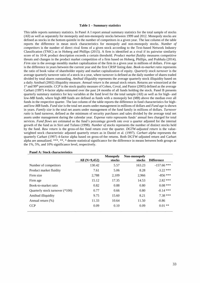
33

Table 1 – Summary statistics

This table reports summary statistics. In Panel A I report annual summary statistics for the total sample of stocks

(All) as well as separately for monopoly and non-monopoly stocks between 1999 and 2012. Monopoly stocks are

defined as stocks in the bottom quintile in the number of competitors in a given year. The last column of the table

reports the difference in mean stock characteristics for monopoly and non-monopoly stocks. Number of

competitors is the number of direct rival firms of a given stock according to the Text-based Network Industry

Classification (TNIC) as in Hoberg and Phillips (2015). A firm is identified as a rival if its pairwise similarity

score of its 10-K product description exceeds a certain threshold. Product market fluidity measures competitive

threats and changes in the product market competition of a firm based on Hoberg, Phillips, and Prabhala (2014).

Firm size is the average monthly market capitalization of the firm in a given year in millions of dollars. Firm age

is the difference in years between the current year and the first CRSP listing date. Book-to-market ratio represents

the ratio of book value of shareholder equity and market capitalization of equity. Quarterly stock turnover is the

average quarterly turnover ratio of a stock in a year, where turnover is defined as the daily number of shares traded

divided by total shares outstanding. Amihud illiquidity represents the average quarterly stock illiquidity based on

a daily Amihud (2002) illiquidity measure. Annual return is the annual stock return. Returns are winsorized at the

1st and 99th percentile. CCP is the stock quality measure of Cohen, Coval, and Pastor (2005) defined as the average

Carhart (1997) 4-factor alpha estimated over the past 24 months of all funds holding the stock. Panel B presents

quarterly summary statistics for key variables at the fund level for the total sample (All) as well as for high- and

low-MB funds, where high-MB funds are defined as funds with a monopoly bet (MB) above the median over all

funds in the respective quarter. The last column of the table reports the difference in fund characteristics for high-

and low-MB funds. Fund size is the total net assets under management in millions of dollars and Fund age is shown

in years. Family size is the total net assets under management of the fund family in millions of dollars. Turnover

ratio is fund turnover, defined as the minimum of security purchases and sales divided by the average total net

assets under management during the calendar year. Expense ratio represents funds’ annual fees charged for total

services. Fund flows are estimated as the fund’s percentage growth rate over a quarter adjusted for the internal

growth of the fund as in Sirri and Tufano (1998). Number of stocks represents the number of distinct stocks held

by the fund. Raw return is the gross-of-fee fund return over the quarter. DGTW-adjusted return is the value-

weighted stock characteristic adjusted quarterly return as in Daniel et al. (1997). Carhart alpha represents the

quarterly Carhart (1997) 4-factor alpha based on gross-of-fee returns. Both DGTW-adjusted return and Carhart

alpha are annualized. ***, **, * denote statistical significance for the difference in means between both groups at

the 1%, 5%, and 10% significance level, respectively.

Panel A: Stock characteristics

All (N=9,452)

Monopoly

stocks

Non-monopoly

stocks Difference

Number of competitors 130.42 5.57 163.23 -157.66 ***

Product market fluidity 7.61 5.06 8.28 -3.22 ***

Firm size 2,788 2,109 2,966 -856 ***

Firm age 15.12 17.35 14.53 2.82 ***

Book-to-market ratio 0.82 0.88 0.80 0.08 ***

Quarterly stock turnover (*100) 0.77 0.66 0.80 -0.14 ***

Amihud illiquidity 9.75 15.60 8.21 7.38 ***

Annual return (%) 11.33 10.64 11.50 -0.86

CCP 0.09 0.10 0.09 0.01 **

34

Table 1 – Summary statistics (continued)

Panel B: Fund characteristics

All (N=2,561) High-MB Low-MB Difference

Fund size 1,353 1,180 1,526 -346 ***

Fund age 14.81 14.68 14.95 -0.27 ***

Turnover ratio (%) 87.09 79.20 95.02 -15.82 ***

Expense ratio (%) 1.30 1.31 1.29 0.02 **

Fund flows (%) 2.24 2.71 1.76 0.95 ***

Number of stocks 111.68 114.17 109.18 4.99 ***

Family size 23,961 21,775 26,166 -4,391 ***

Raw return (%) 3.72 4.48 2.98 1.50 ***

DGTW-adjusted return (%) 0.19 0.64 -0.27 0.91 ***

Carhart alpha (%), gross 0.23 0.62 -0.16 0.78 ***

35

Table 2 – MB and a fund’s reaction to product market competition

This table presents results from pooled OLS regressions that analyze the relation between a fund’s response to a

firm’s product market competition. In Panel A, the dependent variable is Sensitivity, the R2 from the regression of

annual changes in a fund’s holdings of a given stock on changes in the number of competitors of the stock in the

previous two years. The main independent variable is the fund’s monopoly bet (MB). MB is the value-weighted

fraction of monopoly firms in the fund portfolio at a given report date adjusted for the average portfolio weight in

monopoly firms over all funds in the same investment style. I run separate regressions for the continuous variable

as well as for the high-MB dummy, which is equal to one if the fund’s MB is above the median in a given period,

and zero otherwise. Additional independent controls include fund size, fund age, turnover ratio, expense ratio,

fund flows, number of stocks, and family size. Fund size is the logarithm of total net assets under management in

millions of dollars and Fund age is the logarithm of a fund’s age in years. Turnover ratio is fund turnover, defined

as the minimum of security purchases and sales divided by the average total net assets under management during

the calendar year. Expense ratio represents funds’ annual fees charged for total services. Fund flows are estimated

as the fund’s percentage growth rate over a quarter adjusted for the internal growth of the fund as in Sirri and

Tufano (1998). Number of stocks represents the logarithm of the number of distinct stocks held by the fund. Family

size is the logarithm of total net assets under management of the fund family in millions of dollars. All independent

variables are valid at the beginning of the year, for which I calculate Sensitivity. If not indicated otherwise,

regressions are run with time and style fixed effects and p-values (reported in parentheses) are based on standard

errors are clustered at the fund level. In the first two columns of Panel B, the dependent variable is the value-

weighted number of direct competitors of the stock concurrently held by the fund in the non-monopoly stock

portfolio in a given quarter. In the last two columns of Panel B, the dependent variable is the trade-size-weighted

number of direct competitors concurrently bought in the non-monopoly stock portfolio. Both dependent variables

are peer-adjusted by deducting the mean value per investment style and period. The independent variables are the

same as in Panel A, but now valid as of the end of the quarter preceding the calculation of the dependent variables.

Regressions are run with time and style fixed effects. p-values reported in parentheses are based on standard errors

clustered by fund. ***, **, * denote statistical significance at the 1%, 5%, and 10% significance level, respectively.

Panel A: Sensitivity to changes in the number of competitors

Dependent variable: Sensitivity Sensitivity

Monopoly bet (MB) 0.0526 *** 0.0197 ***

(0.0000) (0.0047)

High MB 0.0040 *** 0.0017 ***

(0.0000) (0.0072)

Fund size 0.0004 * 0.0004 *

(0.0922) (0.0903)

Fund age -0.0008 -0.0008

(0.1167) (0.1087)

Turnover ratio -0.0030 *** -0.0031 ***

(0.0000) (0.0000)

Expense ratio 0.0284 0.0308

(0.3907) (0.3405)

Fund flows 0.0023 0.0023

(0.2550) (0.2521)

Number of stocks -0.0192 *** -0.0193 ***

(0.0000) (0.0000)

Family size -0.0004 *** -0.0004 ***

(0.0017) (0.0011)

Time fixed effects No Yes No Yes

Style fixed effects No Yes No Yes

Number of observations 14,507 13,447 14,507 13,447

Adj. R-Squared 0.0070 0.1585 0.0027 0.1580

36

Table 2 – MB and a fund’s reaction to product market competition (continued)

Panel B: Concurrent holding and trading of direct competitors

(Peer-adjusted) Average number of competitors concurrently

Dependent variable: Held Bought

Monopoly bet (MB) -2.9878 *** -1.2959 ***

(0.0000) (0.0000)

High MB -0.4044 *** -0.2132 ***

(0.0000) (0.0000)

Fund size 0.0337 0.0318 0.0507 *** 0.0495 ***

(0.3124) (0.3404) (0.0003) (0.0004)

Fund age -0.3840 *** -0.3819 *** -0.2956 *** -0.2944 ***

(0.0003) (0.0003) (0.0000) (0.0000)

Turnover ratio -0.3654 *** -0.3588 *** 0.1694 *** 0.1688 ***

(0.0003) (0.0004) (0.0000) (0.0000)

Expense ratio 6.8371 6.4127 -2.3794 -2.5328

(0.4024) (0.4270) (0.3856) (0.3535)

Fund flows 0.1816 *** 0.1814 *** 0.4151 *** 0.4150 ***

(0.0002) (0.0002) (0.0000) (0.0000)

Number of stocks 5.4279 *** 5.4440 *** 2.1660 *** 2.1734 ***

(0.0000) (0.0000) (0.0000) (0.0000)

Family size -0.1377 *** -0.1352 *** -0.0309 *** -0.0303 ***

(0.0000) (0.0000) (0.0006) (0.0008)

Time fixed effects Yes Yes Yes Yes

Style fixed effects Yes Yes Yes Yes

Number of observations 54,517 54,517 53,956 53,956

Adj. R-Squared 0.5206 0.5206 0.3877 0.3884

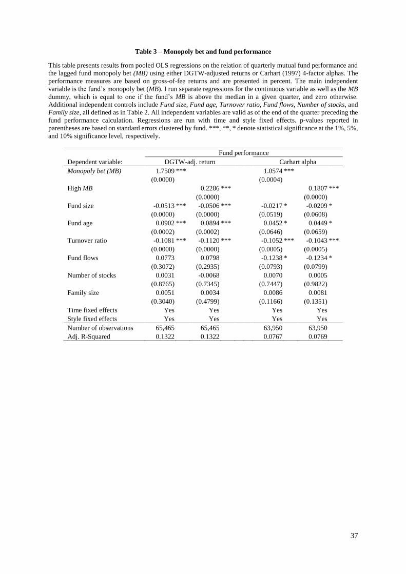
37

Table 3 – Monopoly bet and fund performance

This table presents results from pooled OLS regressions on the relation of quarterly mutual fund performance and

the lagged fund monopoly bet (MB) using either DGTW-adjusted returns or Carhart (1997) 4-factor alphas. The

performance measures are based on gross-of-fee returns and are presented in percent. The main independent

variable is the fund’s monopoly bet (MB). I run separate regressions for the continuous variable as well as the MB

dummy, which is equal to one if the fund’s MB is above the median in a given quarter, and zero otherwise.

Additional independent controls include Fund size, Fund age, Turnover ratio, Fund flows, Number of stocks, and

Family size, all defined as in Table 2. All independent variables are valid as of the end of the quarter preceding the

fund performance calculation. Regressions are run with time and style fixed effects. p-values reported in

parentheses are based on standard errors clustered by fund. ***, **, * denote statistical significance at the 1%, 5%,

and 10% significance level, respectively.

Fund performance

Dependent variable: DGTW-adj. return Carhart alpha

Monopoly bet (MB) 1.7509 *** 1.0574 ***

(0.0000) (0.0004)

High MB 0.2286 *** 0.1807 ***

(0.0000) (0.0000)

Fund size -0.0513 *** -0.0506 *** -0.0217 * -0.0209 *

(0.0000) (0.0000) (0.0519) (0.0608)

Fund age 0.0902 *** 0.0894 *** 0.0452 * 0.0449 *

(0.0002) (0.0002) (0.0646) (0.0659)

Turnover ratio -0.1081 *** -0.1120 *** -0.1052 *** -0.1043 ***

(0.0000) (0.0000) (0.0005) (0.0005)

Fund flows 0.0773 0.0798 -0.1238 * -0.1234 *

(0.3072) (0.2935) (0.0793) (0.0799)

Number of stocks 0.0031 -0.0068 0.0070 0.0005

(0.8765) (0.7345) (0.7447) (0.9822)

Family size 0.0051 0.0034 0.0086 0.0081

(0.3040) (0.4799) (0.1166) (0.1351)

Time fixed effects Yes Yes Yes Yes

Style fixed effects Yes Yes Yes Yes

Number of observations 65,465 65,465 63,950 63,950

Adj. R-Squared 0.1322 0.1322 0.0767 0.0769

38

Table 4 – Performance of buys in monopoly and non-monopoly stocks

This table presents results from pooled OLS regressions on the relation of quarterly performance of buy sub-portfolios in monopoly and non-monopoly stocks and the lagged

monopoly bet (MB). Monopoly stocks are defined as stocks in the bottom quintile according to the number of competitors in a given year. Stocks in the remaining quintiles are part

of the non-monopoly stock portfolio. In Panel A, the dependent variable is the next-quarter performance of a sub-portfolio consisting of a fund’s stock purchases in a given quarter.

I define a purchase as an increase in the number of shares held by a fund in a stock between two consecutive reporting dates. Sub-portfolio performance is measured using DGTW-

adjusted returns and Carhart (1997) 4-factor alphas of the stocks. The performance is presented in percent. I value-weight the performance of stocks making up each sub-portfolio

by the dollar value of the trade (stock price times the number of shares bought or sold of a given stock). In Panel B, the dependent variable is the performance difference between

the buy sub-portfolio of Panel A and a hypothetical portfolio in which the dollar value spent for the actual purchase is equally split over the stock’s rival firms as identified in the

TNIC data. The main independent variable in both Panels is the fund’s monopoly bet (MB). I run separate regressions for the continuous variable as well as the MB dummy, which

is equal to one if the fund’s MB is above the median in a given quarter, and zero otherwise. Additional independent controls are as in Table 3 and suppressed in Panel B of the table.

The independent variables are valid at the end of the quarter preceding the sub-portfolio performance calculation. Regressions are run with time and style fixed effects and standard

errors are clustered by fund. ***, **, * denote statistical significance at the 1%, 5%, and 10% significance level, respectively.

39

Table 4 – Performance of buys in monopoly and non-monopoly stocks (continued)

Panel A: Performance of buy sub-portfolios

Monopoly buys Non-monopoly buys

Dependent variable: DGTW-adj. return Carhart alpha DGTW-adj. return Carhart alpha

Monopoly bet (MB) 2.3871 *** 1.5400 * 2.0515 *** 1.3095 **

(0.0020) (0.0796) (0.0000) (0.0263)

High MB 0.3016 *** 0.2078 ** 0.3162 *** 0.2035 ***

(0.0005) (0.0337) (0.0000) (0.0005)

Fund size -0.0249 -0.0234 0.0132 0.0143 -0.0536 *** -0.0523 *** -0.0528 ** -0.0519 **

(0.4136) (0.4434) (0.7084) (0.6851) (0.0021) (0.0028) (0.0188) (0.0206)

Fund age -0.0099 -0.0121 -0.0208 -0.0223 0.0656 0.0642 0.1022 ** 0.1013 **

(0.8862) (0.8612) (0.7893) (0.7753) (0.1169) (0.1252) (0.0367) (0.0383)

Turnover ratio -0.0947 -0.0998 -0.2105 *** -0.2127 *** -0.1886 *** -0.1889 *** -0.2495 *** -0.2496 ***

(0.1672) (0.1433) (0.0050) (0.0047) (0.0000) (0.0000) (0.0000) (0.0000)

Fund flows 0.2175 * 0.2195 * 0.0152 0.0166 0.2275 ** 0.2300 ** 0.1316 0.1332

(0.0610) (0.0589) (0.9036) (0.8946) (0.0313) (0.0309) (0.2361) (0.2316)

Number of stocks -0.0387 -0.0577 -0.1573 ** -0.1694 *** -0.0596 -0.0710 * -0.1671 *** -0.1743 ***

(0.5025) (0.3125) (0.0162) (0.0095) (0.1035) (0.0521) (0.0002) (0.0001)

Family size -0.0050 -0.0076 0.0037 0.0022 -0.0026 -0.0038 -0.0160 -0.0168

(0.7570) (0.6396) (0.8459) (0.9073) (0.7986) (0.7069) (0.1942) (0.1708)

Time fixed effects Yes Yes Yes Yes Yes Yes Yes Yes

Style fixed effects Yes Yes Yes Yes Yes Yes Yes Yes

Number of

observations 58,331 58,331 58,192 58,192 64,359 64,359 64,335 64,335

Adj. R-Squared 0.0252 0.0252 0.0272 0.0272 0.0408 0.0410 0.0318 0.0319

40

Table 4 – Performance of buys in monopoly and non-monopoly stocks (continued)

Panel B: Performance relative to a firm's rivals

Monopoly buys Non-monopoly buys

Dependent variable: Diff. DGTW Diff. Carhart Diff. DGTW Diff. Carhart

Monopoly bet (MB) 1.8964 ** 1.3969 1.1080 ** 1.8982 ***

(0.0214) (0.1333) (0.0169) (0.0007)

High MB 0.2602 *** 0.2007 * 0.2072 *** 0.2552 ***

(0.0055) (0.0627) (0.0000) (0.0000)

Controls Yes Yes Yes Yes Yes Yes Yes Yes

Time fixed effects Yes Yes Yes Yes Yes Yes Yes Yes

Style fixed effects Yes Yes Yes Yes Yes Yes Yes Yes

Number of observations 58,270 58,270 58,025 58,025 64,359 64,359 64,329 64,329

Adj. R-Squared 0.0204 0.0204 0.0340 0.0340 0.0737 0.0738 0.1534 0.1534

41

Table 5 – Robustness

This table presents robustness checks for the baseline regression of Table 3. For brevity, I only report coefficients

of interest and suppress control variables. If not indicated otherwise, fund performance is measured using DGTW-

adjusted returns or Carhart (1997) 4-factor alphas based on gross-of-fee returns and reported in percent. The main

independent variables are the monopoly bet (MB) or the MB dummy, defined as in Table 2. In Panel A, I vary the

performance measurement. I use the Jensen (1968) 1-factor, the Fama and French (1993) 3-factor, the Pástor and

Stambaugh (2003) 5-factor, as well as the Cremers, Petajisto, and Zitzewitz (2012) 4-and 7-factor models to

estimate fund performance. I also calculate a fund’s Cohen, Coval, and Pástor (2005) alpha, which is the value-

weighted average stock quality measure based on the average Carhart (1997) 4-factor alpha of all funds holding a

particular stock. In Panel B, I modify the empirical approach by using fund fixed effects, manager fixed effects,

family-time fixed effects, or style-time fixed effects. In addition, I report results of a permutation test where the

MB and the high-MB dummy are randomly assigned to funds and the baseline regression of Table 3 is rerun. I

repeat the permutation 10,000 times. p-values of this exercise (reported in parentheses) are equal to the fraction of

permutations that show an effect that is as strong as the performance difference observed in Table 3. Finally, the

last row of Panel B presents results of a weighted matched sample where weights are based on a propensity score

matching. To calculate propensity scores, I estimate a logistic regression of the high-MB dummy on the same

control variables as in the baseline regression as well as time and style fixed effects. In Panel C, I construct

alternative measures to capture a fund’s tendency to invest in stocks with few competitors and repeat the pooled

regression of Table 3 using these alternative proxies. I calculate the equally-weighted instead of the value-weighted

fraction of monopoly stocks, the value-weighted average number of competitors of all firms in the portfolio, the

value-weighted fraction of stocks in the bottom quintile of product market fluidity, and the value-weighted product

market fluidity of all stocks in the portfolio. If not indicated otherwise, the regressions include style and time fixed

effects and p-values reported in parentheses are based on standard errors clustered by fund. ***, **, * denote

statistical significance at the 1%, 5%, and 10% significance level, respectively.

Panel A: Alternative performance measures

MB High MB

Jensen alpha 2.2015 *** 0.2714 ***

(0.0000) (0.0000)

Fama-French alpha 0.8726 *** 0.1413 ***

(0.0041) (0.0000)

Pastor-Stambaugh alpha 0.8688 *** 0.1506 ***

(0.0037) (0.0000)

CPZ-4-factor alpha 1.4967 *** 0.2283 ***

(0.0000) (0.0000)

CPZ-7-factor alpha 1.1681 *** 0.1650 ***

(0.0001) (0.0000)

CCP-4-factor alpha 0.0621 *** 0.0073 ***

(0.0019) (0.0000)

42

Table 5 – Robustness (continued)

Panel B: Estimation method

DGTW-adj. return Carhart alpha

MB High MB MB High MB

Fund fixed effects 1.3874 *** 0.1760 *** 0.7687 ** 0.1419 ***

(0.0009) (0.0000) (0.0440) (0.0000)

Manager fixed effects 0.9876 ** 0.1749 *** 0.7884 * 0.1294 ***

(0.0353) (0.0000) (0.0526) (0.0004)

Family-time fixed effects 1.7223 *** 0.1683 *** 0.8317 *** 0.1447 ***

(0.0000) (0.0000) (0.0026) (0.0000)

Style-time fixed effects 1.7430 *** 0.2293 *** 1.0490 *** 0.1721 ***

(0.0000) (0.0000) (0.0004) (0.0000)

Permutation 1.7509 *** 0.2286 *** 1.0574 *** 0.1807 ***

(0.0000) (0.0000) (0.0004) (0.0000)

Matched sample 0.1911 *** 0.2274 ***

(0.0000) (0.0000)

Panel C: Alternative proxies

DGTW-adj. return Carhart alpha

Continuous

measure

Above median

cutoff

Continuous

measure

Above median

cutoff

Equally-weighted monopoly stocks 1.7987 *** 0.2186 *** 1.0770 *** 0.1535 ***

(0.0000) (0.0000) (0.0007) (0.0000)

Value-weighted number of competitors -0.0074 *** -0.2519 *** -0.0051 *** -0.2143 ***

(0.0000) (0.0000) (0.0000) (0.0000)

Monopoly by product market fluidity 2.6854 *** 0.3462 *** 1.2581 *** 0.1328 ***

(0.0000) (0.0000) (0.0000) (0.0000)

Value-weighted product market fluidity -0.3349 *** -0.4464 *** -0.1924 *** -0.2122 ***

(0.0000) (0.0000) (0.0000) (0.0000)

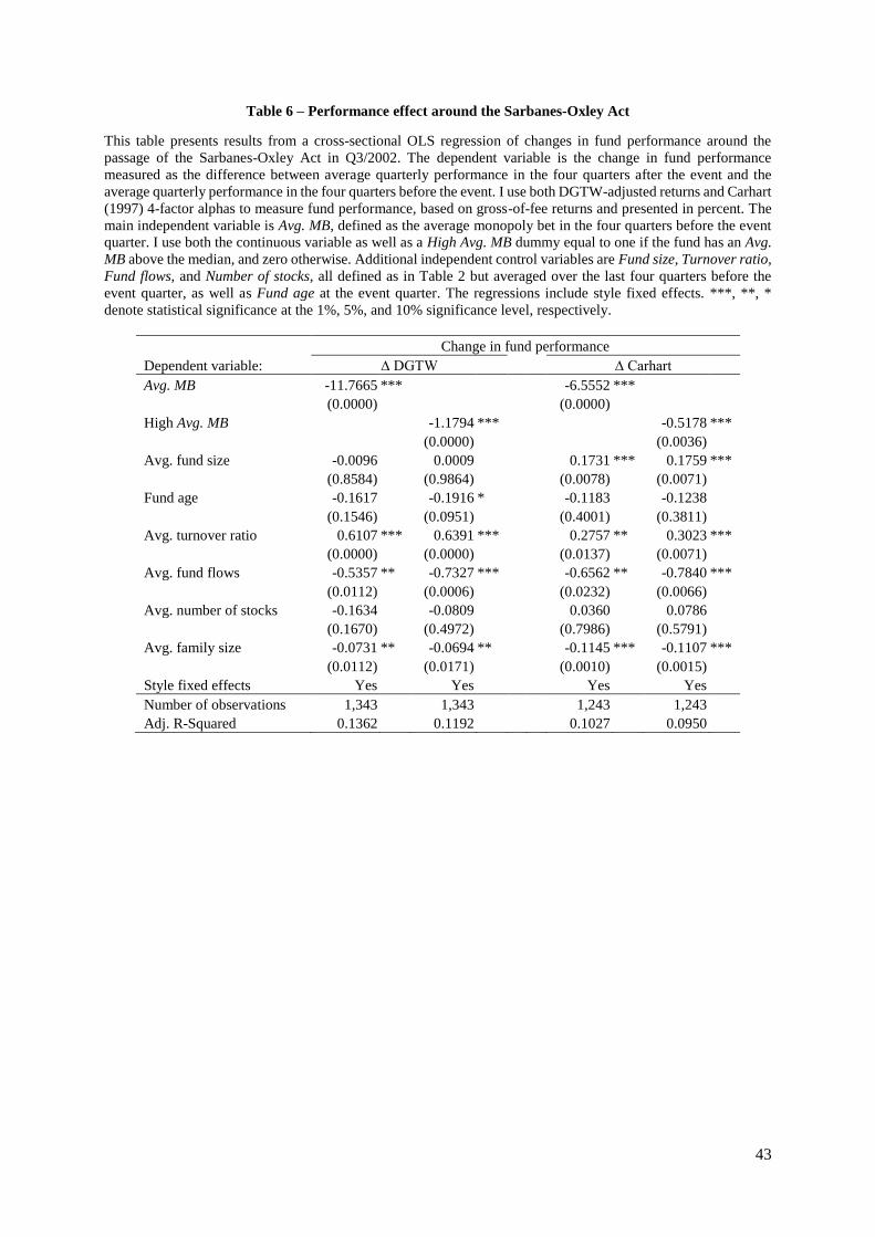
43

Table 6 – Performance effect around the Sarbanes-Oxley Act

This table presents results from a cross-sectional OLS regression of changes in fund performance around the

passage of the Sarbanes-Oxley Act in Q3/2002. The dependent variable is the change in fund performance

measured as the difference between average quarterly performance in the four quarters after the event and the

average quarterly performance in the four quarters before the event. I use both DGTW-adjusted returns and Carhart

(1997) 4-factor alphas to measure fund performance, based on gross-of-fee returns and presented in percent. The

main independent variable is Avg. MB, defined as the average monopoly bet in the four quarters before the event

quarter. I use both the continuous variable as well as a High Avg. MB dummy equal to one if the fund has an Avg.

MB above the median, and zero otherwise. Additional independent control variables are Fund size, Turnover ratio,

Fund flows, and Number of stocks, all defined as in Table 2 but averaged over the last four quarters before the

event quarter, as well as Fund age at the event quarter. The regressions include style fixed effects. ***, **, *

denote statistical significance at the 1%, 5%, and 10% significance level, respectively.

Change in fund performance

Dependent variable: ∆ DGTW ∆ Carhart

Avg. MB -11.7665 *** -6.5552 ***

(0.0000) (0.0000)

High Avg. MB -1.1794 *** -0.5178 ***

(0.0000) (0.0036)

Avg. fund size -0.0096 0.0009 0.1731 *** 0.1759 ***

(0.8584) (0.9864) (0.0078) (0.0071)

Fund age -0.1617 -0.1916 * -0.1183 -0.1238

(0.1546) (0.0951) (0.4001) (0.3811)

Avg. turnover ratio 0.6107 *** 0.6391 *** 0.2757 ** 0.3023 ***

(0.0000) (0.0000) (0.0137) (0.0071)

Avg. fund flows -0.5357 ** -0.7327 *** -0.6562 ** -0.7840 ***

(0.0112) (0.0006) (0.0232) (0.0066)

Avg. number of stocks -0.1634 -0.0809 0.0360 0.0786

(0.1670) (0.4972) (0.7986) (0.5791)

Avg. family size -0.0731 ** -0.0694 ** -0.1145 *** -0.1107 ***

(0.0112) (0.0171) (0.0010) (0.0015)

Style fixed effects Yes Yes Yes Yes

Number of observations 1,343 1,343 1,243 1,243

Adj. R-Squared 0.1362 0.1192 0.1027 0.0950

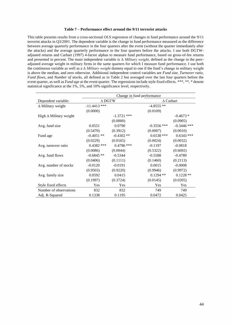
44

Table 7 – Performance effect around the 9/11 terrorist attacks

This table presents results from a cross-sectional OLS regression of changes in fund performance around the 9/11

terrorist attacks in Q3/2001. The dependent variable is the change in fund performance measured as the difference

between average quarterly performance in the four quarters after the event (without the quarter immediately after

the attacks) and the average quarterly performance in the four quarters before the attacks. I use both DGTW-

adjusted returns and Carhart (1997) 4-factor alphas to measure fund performance, based on gross-of-fee returns

and presented in percent. The main independent variable is ∆ Military weight, defined as the change in the peer-

adjusted average weight in military firms in the same quarters for which I measure fund performance. I use both

the continuous variable as well as a ∆ Military weight dummy equal to one if the fund’s change in military weight

is above the median, and zero otherwise. Additional independent control variables are Fund size, Turnover ratio,

Fund flows, and Number of stocks, all defined as in Table 2 but averaged over the last four quarters before the

event quarter, as well as Fund age at the event quarter. The regressions include style fixed effects. ***, **, * denote

statistical significance at the 1%, 5%, and 10% significance level, respectively.

Change in fund performance

Dependent variable: ∆ DGTW ∆ Carhart

∆ Military weight -11.4413 *** -4.8555 **

(0.0000) (0.0109)

High ∆ Military weight -1.3721 *** -0.4673 *

(0.0000) (0.0905)

Avg. fund size 0.0551 0.0790 -0.3556 *** -0.3446 ***

(0.5470) (0.3912) (0.0007) (0.0010)

Fund age -0.4051 ** -0.4302 ** 0.6538 *** 0.6343 ***

(0.0229) (0.0165) (0.0024) (0.0032)

Avg. turnover ratio 0.4382 *** 0.4786 *** -0.1197 -0.0818

(0.0086) (0.0044) (0.5322) (0.6692)

Avg. fund flows -0.6845 ** -0.5344 -0.5588 -0.4789

(0.0406) (0.1111) (0.1460) (0.2113)

Avg. number of stocks -0.0120 -0.0191 0.0015 -0.0008

(0.9503) (0.9220) (0.9946) (0.9972)

Avg. family size 0.0592 0.0415 0.1294 ** 0.1228 **

(0.1997) (0.3724) (0.0145) (0.0205)

Style fixed effects Yes Yes Yes Yes

Number of observations 832 832 749 749

Adj. R-Squared 0.1338 0.1195 0.0472 0.0425

45

Table 8 – Impact of manager changes and manager attributes on MB

This table presents results on the influence of the fund manager on a fund’s monopoly bet (MB). Panel A presents

results on changes in monopoly bets around changes in the fund manager for a sub-sample of single-managed

funds. The dependent variable is the change in average monopoly bets (∆ MB), measured as the difference of the

average quarterly MB in the four quarters after the manager change quarter and the average quarterly MB in the

four quarters before the change quarter. The main independent variables are ∆ MB propensity, which is the

difference between the MB propensity of the new manager and the fund’s average MB in the four quarters before

the change, as well as an indicator variable equal to one if this difference is positive, and zero otherwise (I (∆ MB

propensity > 0)). The MB propensity of the new manager is defined as the average MB in the four quarters before

the change across all single- and team-managed funds managed by the new manager. Additional independent

controls are as in Table 2. All independent variables are valid as of the end of the quarter of the manager switch.

In the first column of Panel B, I present results of pooled OLS regressions where the dependent variable is the

monopoly bet for the fund in a given quarter. In the last column of Panel B, I present results of logistic regressions

where the dependent variable is the high-MB dummy, an indicator variable equal to one if the fund has a monopoly

bet above the median of all funds in a given quarter, and zero otherwise. The main independent variables are

multiple funds per manager, manager tenure, and # Managers. Multiple funds per manager is an indicator variable

equal to one, if the fund managers on average manage more than one fund, and zero otherwise. Manager tenure is

the maximum manager tenure in the fund industry over all managers of the fund. # Managers is the number of

managers of the fund. Additional independent control variables are the same as in Table 2. All independent

variables are lagged by one quarter. Regressions are run with time and style fixed effects. p-values reported in

parentheses are based on standard errors clustered by fund. ***, **, * denote statistical significance at the 1%, 5%,

and 10% significance level, respectively.

Panel A: Changes in MB around manager changes

Dependent variable: ∆MB ∆MB

∆ MB propensity 0.3899 ***

(0.0000)

I (∆ MB propensity > 0) 0.0372 ***

(0.0001)

Fund size 0.0015 0.0066

(0.7400) (0.1787)

Fund age 0.0094 -0.0021

(0.3273) (0.8320)

Turnover ratio 0.0035 0.0015

(0.5698) (0.8006)

Expense ratio 0.9159 0.8306

(0.5825) (0.6437)

Fund flows 0.0141 0.0396

(0.6945) (0.3245)

Number of stocks 0.0069 0.0048

(0.2935) (0.4918)

Family size 0.0012 0.0001

(0.6331) (0.9843)

Style fixed effects Yes Yes

Time fixed effects Yes Yes

Number of observations 140 140

Adj. R-Squared 0.4541 0.3708

46

Table 8 – Impact of manager changes and manager attributes on MB (continued)

Panel B: Determinants of MB

Dependent variable: Monopoly bet (MB) High MB

Multiple funds per manager -0.0060 *** -0.1100 *

(0.0074) (0.0601)

Manager tenure 0.0006 *** 0.0154 ***

(0.0013) (0.0003)

# Managers -0.0009 *** -0.0378 ***

(0.0072) (0.0004)

Fund size -0.0010 -0.0443 ***

(0.1816) (0.0087)

Fund age -0.0013 -0.0137

(0.3933) (0.7223)

Turnover ratio -0.0120 *** -0.3057 ***

(0.0000) (0.0000)

Expense ratio 0.0937 0.1718

(0.2526) (0.9338)

Fund flows 0.0006 0.0015

(0.7251) (0.9715)

Number of stocks -0.0037 ** 0.0497

(0.0172) (0.1829)

Family size -0.0022 *** -0.0396 ***

(0.0000) (0.0001)

Time fixed effects Yes Yes

Style fixed effects Yes Yes

Number of observations 52,009 52,009

Adj./Pseudo R-Squared 0.0453 0.0166

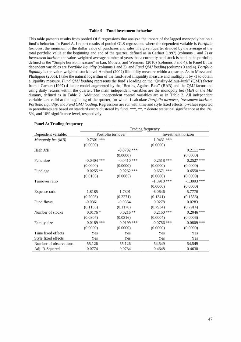
47

Table 9 – Fund investment behavior

This table presents results from pooled OLS regressions that analyze the impact of the lagged monopoly bet on a

fund’s behavior. In Panel A, I report results of pooled OLS regressions where the dependent variable is Portfolio

turnover, the minimum of the dollar value of purchases and sales in a given quarter divided by the average of the

total portfolio value at the beginning and end of the quarter, defined as in Carhart (1997) (columns 1 and 2) or

Investment horizon, the value-weighted average number of years that a currently held stock is held in the portfolio,

defined as the “Simple horizon measure” in Lan, Moneta, and Wermers (2016) (columns 3 and 4). In Panel B, the

dependent variables are Portfolio liquidity (columns 1 and 2), and Fund QMJ loading (columns 3 and 4). Portfolio

liquidity is the value-weighted stock-level Amihud (2002) illiquidity measure within a quarter. As in Massa and

Phalippou (2005), I take the natural logarithm of the fund-level illiquidity measure and multiply it by -1 to obtain

a liquidity measure. Fund QMJ loading represents the fund’s loading on the “Quality-Minus-Junk” (QMJ) factor

from a Carhart (1997) 4-factor model augmented by the “Betting-Against-Beta” (BAB) and the QMJ factor and

using daily returns within the quarter. The main independent variables are the monopoly bet (MB) or the MB

dummy, defined as in Table 2. Additional independent control variables are as in Table 2. All independent

variables are valid at the beginning of the quarter, for which I calculate Portfolio turnover, Investment horizon,

Portfolio liquidity, and Fund QMJ loading. Regressions are run with time and style fixed effects. p-values reported

in parentheses are based on standard errors clustered by fund. ***, **, * denote statistical significance at the 1%,

5%, and 10% significance level, respectively.

Panel A: Trading frequency

Trading frequency

Dependent variable: Portfolio turnover Investment horizon

Monopoly bet (MB) -0.7301 *** 1.9431 ***

(0.0000) (0.0000)

High MB -0.0782 *** 0.2111 ***

(0.0000) (0.0000)

Fund size -0.0404 *** -0.0410 *** 0.2518 *** 0.2527 ***

(0.0000) (0.0000) (0.0000) (0.0000)

Fund age 0.0255 ** 0.0262 *** 0.6571 *** 0.6558 ***

(0.0103) (0.0085) (0.0000) (0.0000)

Turnover ratio -1.3910 *** -1.3993 ***

(0.0000) (0.0000)

Expense ratio 1.8185 1.7391 -6.0646 -5.7770

(0.2003) (0.2271) (0.1341) (0.1556)

Fund flows -0.0361 -0.0364 0.0278 0.0283

(0.1155) (0.1176) (0.7934) (0.7914)

Number of stocks 0.0176 * 0.0216 ** 0.2150 *** 0.2046 ***

(0.0807) (0.0316) (0.0004) (0.0006)

Family size 0.0189 *** 0.0199 *** -0.0786 *** -0.0809 ***

(0.0000) (0.0000) (0.0000) (0.0000)

Time fixed effects Yes Yes Yes Yes

Style fixed effects Yes Yes Yes Yes

Number of observations 55,126 55,126 54,549 54,549

Adj. R-Squared 0.0774 0.0734 0.4648 0.4638

48

Table 9 – Fund investment behavior (continued)

Panel B: Investment strategies

Investment strategy

Dependent variable: Portfolio liquidity Fund QMJ loading

Monopoly bet (MB) -4.7907 *** 0.3526 ***

(0.0000) (0.0000)

High MB -0.4156 *** 0.0429 ***

(0.0000) (0.0000)

Fund size 0.0584 *** 0.0573 *** -0.0057 *** -0.0055 ***

(0.0027) (0.0037) (0.0039) (0.0050)

Fund age 0.0080 0.0110 -0.0031 -0.0033

(0.8577) (0.8095) (0.4883) (0.4588)

Turnover ratio 0.0313 0.0601 -0.0641 *** -0.0652 ***

(0.3874) (0.1032) (0.0000) (0.0000)

Expense ratio -30.6955 *** -31.4225 *** -2.5145 *** -2.4568 ***

(0.0000) (0.0000) (0.0002) (0.0004)

Fund flows -0.0969 *** -0.0992 *** -0.0054 -0.0049

(0.0042) (0.0027) (0.2825) (0.3383)

Number of stocks -0.4523 *** -0.4270 *** 0.0134 *** 0.0113 ***

(0.0000) (0.0000) (0.0002) (0.0019)

Family size 0.0757 *** 0.0826 *** -0.0008 -0.0012

(0.0000) (0.0000) (0.4196) (0.2551)

Time fixed effects Yes Yes Yes Yes

Style fixed effects Yes Yes Yes Yes

Number of observations 54,755 54,782 66,569 66,569

Adj. R-Squared 0.5585 0.5585 0.1586 0.1572

49

Market Power in the Portfolio: Product Market Competition and

Mutual Fund Performance

Internet Appendix

September 2016

This Internet Appendix presents additional results to accompany the paper “Market Power in

the Portfolio: Product Market Competition and Mutual Fund Performance”. The contents of the

Appendix are as follows.

Table A.1 reports results on logistic regressions of a fund’s decision to sell or drop a stock

depending on its average similarity with the newly-purchased stocks in a given quarter.

Table A.2 reports performance and performance differences of buy and sell sub-portfolios

between high- and low-MB funds.

Table A.3 estimates the cross-sectional regression of Table 6 using Q4/2005 as a placebo period

and compares the placebo results with the original results of Table 6.

Table A.4 estimates the results of the average investment horizon (Panel A of Table 9)

separately for monopoly- and non-monopoly sub-portfolios.

50

Table A.1 – Replacing competitors

This table presents results of logistic regressions on the relation between a fund’s decision to replace rival firms

and the monopoly bet (MB). The dependent variable is either a Sell (column 1) or a Drop (column 2) dummy

variable equal to one if the fund has decreased the number of shares of a stock in a given quarter or has eliminated

the stock from the portfolio, respectively, and zero otherwise. Sell and Drop are only calculated for non-monopoly

stocks. The main independent variable is the MB dummy as of the end of the previous quarter. The other main

independent variable is Average similarity, which is the average pairwise similarity score of the stock with all

initiating buys in the same period. A higher score indicates a stronger product similarity. Additional independent

controls at the stock level are the annual return, stock turnover, book-to-market ratio, all defined as in Table 1, and

return volatility which is defined as the standard deviation of daily stock returns within a given quarter. Additional

independent controls at the fund level are the same as in Table 2. Regressions are run with Fama-French-48

industry fixed effects, time fixed effects, and style fixed effects. p-values reported in parentheses are based on

standard errors clustered by fund-stock combination. ***, **, * denote statistical significance at the 1%, 5%, and

10% significance level, respectively.

Trade

Dependent variable: Sell Drop

High MB -0.0510 *** -0.0671 ***

(0.0000) (0.0000)

Average similarity 0.6357 *** 0.6692 ***

(0.0000) (0.0000)

High MB *Average similarity 0.5065 *** 0.2842 ***

(0.0000) (0.0001)

Prior quarter return -0.0000 -0.4745 ***

(0.9987) (0.0000)

Stock turnover 8.5957 *** 13.8996 ***

(0.0000) (0.0000)

Market cap 0.0256 *** -0.1273 ***

(0.0000) (0.0000)

Book-to-market ratio -0.0340 *** -0.0229 ***

(0.0000) (0.0000)

Return volatility 0.2458 *** 0.4818 ***

(0.0000) (0.0000)

Fund size -0.0200 *** -0.0323 ***

(0.0000) (0.0000)

Fund age 0.0568 *** 0.0415 ***

(0.0000) (0.0000)

Turnover ratio 0.5350 *** 0.5557 ***

(0.0000) (0.0000)

Expense ratio 2.7975 *** -1.1541 ***

(0.0000) (0.0001)

Fund flows -1.6122 *** -0.0825 ***

(0.0000) (0.0000)

Number of stocks -0.1977 *** -0.2637 ***

(0.0000) (0.0000)

Family size 0.0505 *** 0.0384 ***

(0.0000) (0.0000)

Industry fixed effects Yes Yes

Time fixed effects Yes Yes

Style fixed effects Yes Yes

Number of observations 4,930,058 4,930,058

Pseudo R-Squared 0.0616 0.0637

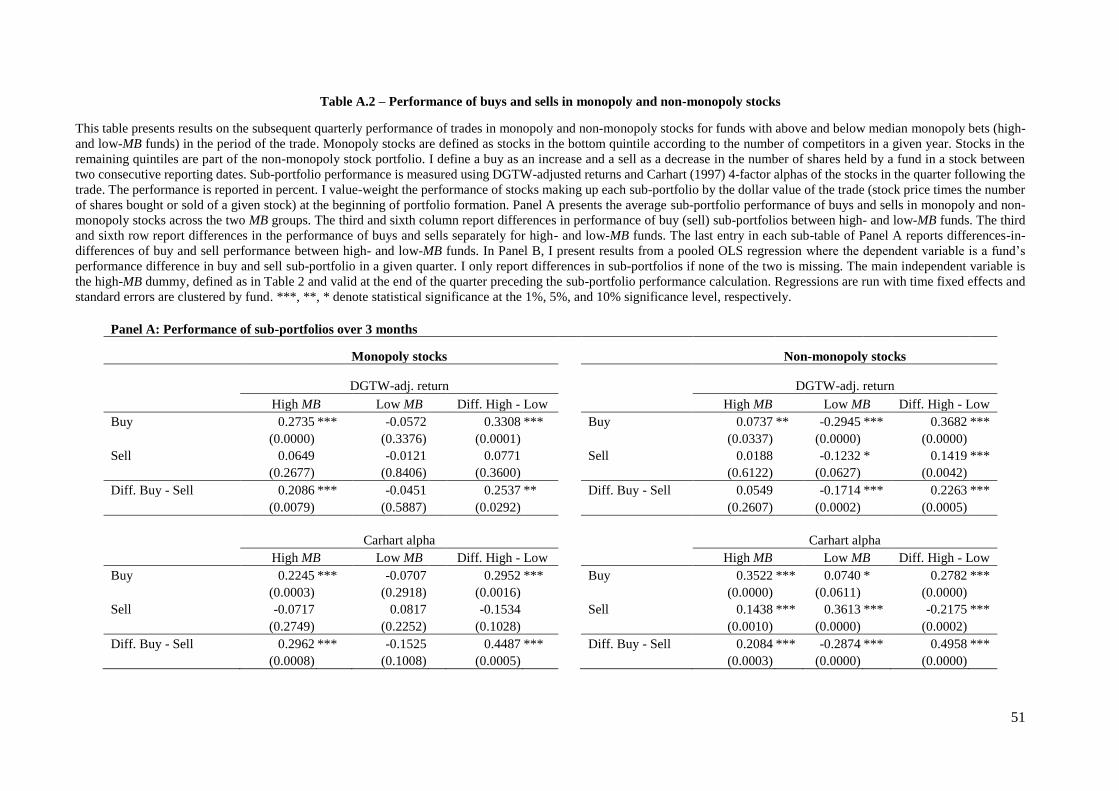
51

Table A.2 – Performance of buys and sells in monopoly and non-monopoly stocks

This table presents results on the subsequent quarterly performance of trades in monopoly and non-monopoly stocks for funds with above and below median monopoly bets (high-

and low-MB funds) in the period of the trade. Monopoly stocks are defined as stocks in the bottom quintile according to the number of competitors in a given year. Stocks in the

remaining quintiles are part of the non-monopoly stock portfolio. I define a buy as an increase and a sell as a decrease in the number of shares held by a fund in a stock between

two consecutive reporting dates. Sub-portfolio performance is measured using DGTW-adjusted returns and Carhart (1997) 4-factor alphas of the stocks in the quarter following the

trade. The performance is reported in percent. I value-weight the performance of stocks making up each sub-portfolio by the dollar value of the trade (stock price times the number

of shares bought or sold of a given stock) at the beginning of portfolio formation. Panel A presents the average sub-portfolio performance of buys and sells in monopoly and non-

monopoly stocks across the two MB groups. The third and sixth column report differences in performance of buy (sell) sub-portfolios between high- and low-MB funds. The third

and sixth row report differences in the performance of buys and sells separately for high- and low-MB funds. The last entry in each sub-table of Panel A reports differences-in-

differences of buy and sell performance between high- and low-MB funds. In Panel B, I present results from a pooled OLS regression where the dependent variable is a fund’s

performance difference in buy and sell sub-portfolio in a given quarter. I only report differences in sub-portfolios if none of the two is missing. The main independent variable is

the high-MB dummy, defined as in Table 2 and valid at the end of the quarter preceding the sub-portfolio performance calculation. Regressions are run with time fixed effects and

standard errors are clustered by fund. ***, **, * denote statistical significance at the 1%, 5%, and 10% significance level, respectively.

Panel A: Performance of sub-portfolios over 3 months

Monopoly stocks Non-monopoly stocks

DGTW-adj. return DGTW-adj. return

High MB Low MB Diff. High - Low High MB Low MB Diff. High - Low

Buy 0.2735 *** -0.0572 0.3308 *** Buy 0.0737 ** -0.2945 *** 0.3682 ***

(0.0000) (0.3376) (0.0001) (0.0337) (0.0000) (0.0000)

Sell 0.0649 -0.0121 0.0771 Sell 0.0188 -0.1232 * 0.1419 ***

(0.2677) (0.8406) (0.3600) (0.6122) (0.0627) (0.0042)

Diff. Buy - Sell 0.2086 *** -0.0451 0.2537 ** Diff. Buy - Sell 0.0549 -0.1714 *** 0.2263 ***

(0.0079) (0.5887) (0.0292) (0.2607) (0.0002) (0.0005)

Carhart alpha Carhart alpha

High MB Low MB Diff. High - Low High MB Low MB Diff. High - Low

Buy 0.2245 *** -0.0707 0.2952 *** Buy 0.3522 *** 0.0740 * 0.2782 ***

(0.0003) (0.2918) (0.0016) (0.0000) (0.0611) (0.0000)

Sell -0.0717 0.0817 -0.1534 Sell 0.1438 *** 0.3613 *** -0.2175 ***

(0.2749) (0.2252) (0.1028) (0.0010) (0.0000) (0.0002)

Diff. Buy - Sell 0.2962 *** -0.1525 0.4487 *** Diff. Buy - Sell 0.2084 *** -0.2874 *** 0.4958 ***

(0.0008) (0.1008) (0.0005) (0.0003) (0.0000) (0.0000)

52

Table A.2 – Performance of buys and sells in monopoly and non-monopoly stocks (continued)

Panel B: Difference-in-differences of sub-portfolio performance

Dependent variable: Difference in buy and sell performance (3 months) Dependent variable: Difference in buy and sell performance (3 months)

DGTW-adj. Carhart alpha DGTW-adj. Carhart alpha High MB 0.2474 ** 0.4445 *** High MB 0.2256 *** 0.4958 ***

(0.0325) (0.0008) (0.0005) (0.0000)

Time fixed effects Yes Yes Time fixed effects Yes Yes

Number of observations 58,798 58,818 Number of observations 70,285 70,263

Adj. R-Squared 0.0013 0.0024 Adj. R-Squared 0.0034 0.0016

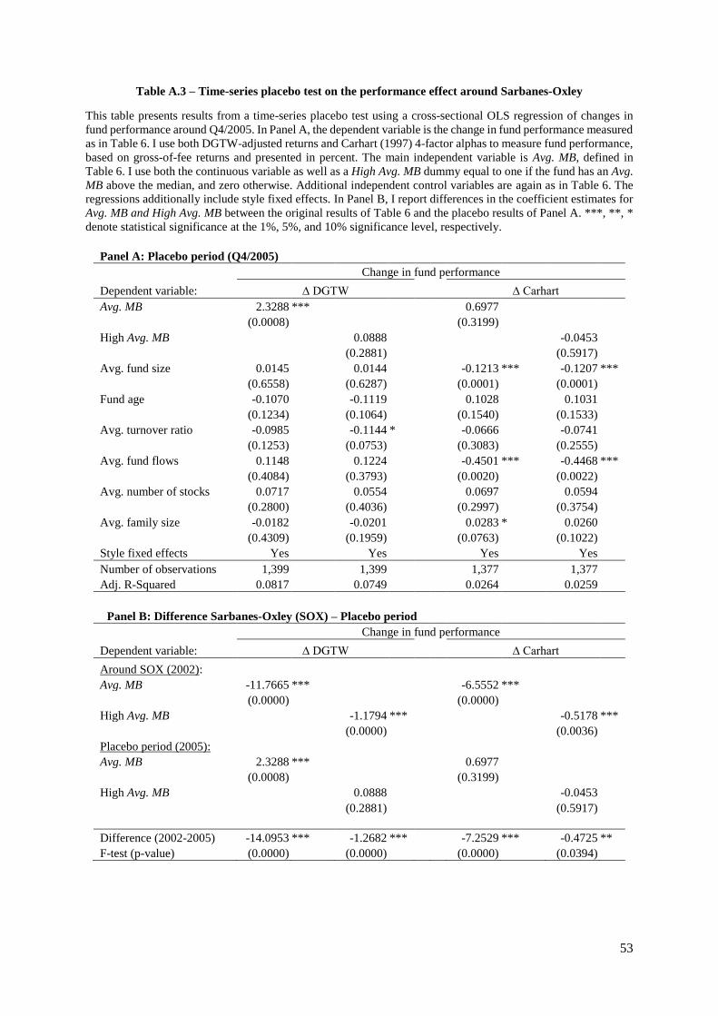
53

Table A.3 – Time-series placebo test on the performance effect around Sarbanes-Oxley

This table presents results from a time-series placebo test using a cross-sectional OLS regression of changes in

fund performance around Q4/2005. In Panel A, the dependent variable is the change in fund performance measured

as in Table 6. I use both DGTW-adjusted returns and Carhart (1997) 4-factor alphas to measure fund performance,

based on gross-of-fee returns and presented in percent. The main independent variable is Avg. MB, defined in

Table 6. I use both the continuous variable as well as a High Avg. MB dummy equal to one if the fund has an Avg.

MB above the median, and zero otherwise. Additional independent control variables are again as in Table 6. The

regressions additionally include style fixed effects. In Panel B, I report differences in the coefficient estimates for

Avg. MB and High Avg. MB between the original results of Table 6 and the placebo results of Panel A. ***, **, *

denote statistical significance at the 1%, 5%, and 10% significance level, respectively.

Panel A: Placebo period (Q4/2005)

Change in fund performance

Dependent variable: ∆ DGTW ∆ Carhart

Avg. MB 2.3288 *** 0.6977

(0.0008) (0.3199)

High Avg. MB 0.0888 -0.0453

(0.2881) (0.5917)

Avg. fund size 0.0145 0.0144 -0.1213 *** -0.1207 ***

(0.6558) (0.6287) (0.0001) (0.0001)

Fund age -0.1070 -0.1119 0.1028 0.1031

(0.1234) (0.1064) (0.1540) (0.1533)

Avg. turnover ratio -0.0985 -0.1144 * -0.0666 -0.0741

(0.1253) (0.0753) (0.3083) (0.2555)

Avg. fund flows 0.1148 0.1224 -0.4501 *** -0.4468 ***

(0.4084) (0.3793) (0.0020) (0.0022)

Avg. number of stocks 0.0717 0.0554 0.0697 0.0594

(0.2800) (0.4036) (0.2997) (0.3754)

Avg. family size -0.0182 -0.0201 0.0283 * 0.0260

(0.4309) (0.1959) (0.0763) (0.1022)

Style fixed effects Yes Yes Yes Yes

Number of observations 1,399 1,399 1,377 1,377

Adj. R-Squared 0.0817 0.0749 0.0264 0.0259

Panel B: Difference Sarbanes-Oxley (SOX) – Placebo period

Change in fund performance

Dependent variable: ∆ DGTW ∆ Carhart

Around SOX (2002):

Avg. MB -11.7665 *** -6.5552 ***

(0.0000) (0.0000)

High Avg. MB -1.1794 *** -0.5178 ***

(0.0000) (0.0036)

Placebo period (2005):

Avg. MB 2.3288 *** 0.6977

(0.0008) (0.3199)

High Avg. MB 0.0888 -0.0453

(0.2881) (0.5917)

Difference (2002-2005) -14.0953 *** -1.2682 *** -7.2529 *** -0.4725 **

F-test (p-value) (0.0000) (0.0000) (0.0000) (0.0394)

54

Table A.4 – Investment horizon in monopoly and non-monopoly sub-portfolios

This table presents results from pooled OLS regressions that analyze the impact of the lagged monopoly bet on a fund’s investment horizon in its monopoly and non-monopoly

sub-portfolios. The dependent variable is the investment horizon measure of a fund in a given quarter, defined as in Table 9. In columns 1 and 2, the investment horizon is measured

for the monopoly sub-portfolios and in columns 3 and 4, it is applied to non-monopoly sub-portfolios. In columns 5 and 6, the dependent variable is the difference between the

average investment horizons in a fund’s monopoly- and non-monopoly sub-portfolios in a given quarter. The main independent variables are the monopoly bet (MB) or the MB

dummy, defined as in Table 2. Additional independent control variables are as in Table 2. All independent variables are valid at the beginning of the quarter, for which I calculate

the investment horizons for the sub-portfolios and the horizon differences. Regressions are run with time and style fixed effects. p-values reported in parentheses are based on

standard errors clustered by fund. ***, **, * denote statistical significance at the 1%, 5%, and 10% significance level, respectively.

Investment horizon

Dependent variable:

Monopoly stocks

Non-monopoly stocks Horizon difference

Monopoly bet (MB) 4.3981 *** 1.7650 *** 2.6333 ***

(0.0000) (0.0002) (0.0000)

High MB 0.4830 *** 0.1784 *** 0.3047 ***

(0.0000) (0.0001) (0.0000)

Fund size 0.2497 *** 0.2519 *** 0.2515 *** 0.2523 *** -0.0019 -0.0005

(0.0000) (0.0000) (0.0000) (0.0000) (0.8864) (0.9734)

Fund age 0.6843 *** 0.6812 *** 0.6450 *** 0.6438 *** 0.0395 0.0376

(0.0000) (0.0000) (0.0000) (0.0000) (0.2814) (0.3037)

Turnover ratio -1.4163 *** -1.4329 *** -1.4098 *** -1.4177 *** -0.0066 -0.0153

(0.0000) (0.0000) (0.0000) (0.0000) (0.7340) (0.4330)

Expense ratio -7.1197 -6.3002 -7.4646 -7.1303 0.3425 0.8281

(0.1063) (0.1565) (0.1057) (0.1234) (0.7957) (0.5247)

Fund flows 0.0312 0.0328 0.0302 0.0309 0.0011 0.0020

(0.7896) (0.7828) (0.7739) (0.7702) (0.9554) (0.9252)

Number of stocks 0.2469 *** 0.2191 *** 0.2477 *** 0.2365 *** -0.0006 -0.0172

(0.0001) (0.0005) (0.0000) (0.0001) (0.9820) (0.5227)

Family size -0.0712 *** -0.0766 *** -0.0781 *** -0.0805 *** 0.0069 0.0039

(0.0000) (0.0000) (0.0000) (0.0000) (0.3514) (0.6082)

Time fixed effects Yes Yes Yes Yes Yes Yes

Style fixed effects Yes Yes Yes Yes Yes Yes

Number of observations 54,251 54,251 54,246 54,246 54,246 54,246

Adj. R-Squared 0.3903 0.3866 0.4638 0.4628 0.0350 0.0315

CFR WCFR WCFR WCFR Working orking orking orking Paper SPaper SPaper SPaper Serieserieserieseries

Centre for Financial ResearchCentre for Financial ResearchCentre for Financial ResearchCentre for Financial Research CologneCologneCologneCologne

CFR Working Papers are available for download from www.cfrwww.cfrwww.cfrwww.cfr----cologne.decologne.decologne.decologne.de. Hardcopies can be ordered from: Centre for Financial Research (CFR), Albertus Magnus Platz, 50923 Koeln, Germany. 2016201620162016 No. Author(s) Title 16-08 S. Kanne, O. Korn,

M.Uhrig-Homburg

Stock Illiquidity, Option Prices and Option Returns

16-07 S. Jaspersen Market Power in the Portfolio: Product Market Competition and Mutual Fund Performance

16-06 O. Korn, M.-O. Rieger

Hedging With Regret

16-05 E. Theissen, C. Westheide

Call of Duty: Designated Market Maker Participation in Call Auctions

16-04 P. Gomber, S. Sagade, E. Theissen, M.C. Weber, C. Westheide

Spoilt for Choice: Order Routing Decisions in Fragmented Equity Markets

16-03 T.Martin, F. Sonnenburg Managerial Ownership Changes and Mutual Fund Performance

16-02

A.Gargano, A. G. Rossi, R. Wermers

The Freedom of Information Act and the Race Towards Information Acquisition

16-01 G. Cici, S. Gibson, C. Rosenfeld

Cross-Company Effects of Common Ownership: Dealings Between Borrowers and Lenders With a Common Blockholder

2015201520152015 No. Author(s) Title 15-17 O. Korn, L. Kuntz Low-Beta Investment Strategies

15-16 D. Blake, A.G. Rossi, A.

Timmermann, I. Tonks, R. Wermers

Network Centrality and Pension Fund Performance

15-15 S. Jank, E. Smajbegovic Dissecting Short-Sale Performance: Evidence from Large Position Disclosures

15-14 M. Doumet, P. Limbach, E. Theissen

Ich bin dann mal weg: Werteffekte von Delistings deutscher Aktiengesellschaften nach dem Frosta-Urteil

15-13 G. Borisova, P.K. Yadav Government Ownership, Informed Trading and Private Information

15-12 V. Agarwal, G.O. Aragon, Z. Shi

Funding Liquidity Risk of Funds of Hedge Funds: Evidence from their Holdings

15-11

L. Ederington, W. Guan, P.K. Yadav

Dealer spreads in the corporate Bond Market: Agent vs. Market-Making Roles

15-10 J.R. Black, D. Stock, P.K. Yadav

The Pricing of Different Dimensions of Liquidity: Evidence from Government Guaranteed Bank Bonds

15-09 15-08 15-07 15-06 15-05 15-04

V. Agarwal, H. Zhao V. Agarwal, T. C. Green, H. Ren V. Agarwal, S. Ruenzi, F. Weigert C. Lan, F. Moneta, R. Wermers L.K. Dahm, C. Sorhage A. Kempf, D. Mayston, M. Gehde-Trapp, P. K. Yadav

Interfund lending in mutual fund families: Role of internal capital markets Alpha or Beta in the Eye of the Beholder: What drives Hedge Fund Flows? Tail risk in hedge funds: A unique view from portfolio holdings Mutual Fund Investment Horizon and Performance Milk or Wine: Mutual Funds’ (Dis)economies of Life Resiliency: A Dynamic View of Liquidity

15-03

V. Agarwal, Y. E. Arisoy, N. Y. Naik

Volatility of Aggregate Volatility and Hedge Funds Returns

15-02

G. Cici, S. Jaspersen, A. Kempf

Speed of Information Diffusion within Fund Families

15-01 M. Baltzer, S. Jank, E. Smajlbegovic

Who trades on momentum?

2014201420142014 No. Author(s) Title 14-15

M. Baltzer, S. Jank, E.Smajlbegovic

Who Trades on Monumentum?

14-14

G. Cici, L. K. Dahm, A. Kempf

Trading Efficiency of Fund Families: Impact on Fund Performance and Investment Behavior

14-13 V. Agarwal, Y. Lu, S. Ray Under one roof: A study of simultaneously managed hedge funds and funds of hedge funds

14-12 P. Limbach, F. Sonnenburg

Does CEO Fitness Matter?

14-11 G. Cici, M. Gehde-Trapp, M. Göricke, A. Kempf

What They Did in their Previous Life: The Investment Value of Mutual Fund Managers’ Experience outside the Financial Sector

14-10 O. Korn, P. Krischak, E. Theissen

Illiquidity Transmission from Spot to Futures Markets

14-09 E. Theissen, L. S. Zehnder Estimation of Trading Costs: Trade Indicator Models Revisited

14-08 C. Fink, E. Theissen Dividend Taxation and DAX Futures Prices

14-07 F. Brinkmann, O. Korn Risk-adjusted Option-implied Moments

14-06 J. Grammig, J. Sönksen Consumption-Based Asset Pricing with Rare Disaster Risk

14-05 J. Grammig, E. Schaub Give me strong moments and time – Combining GMM and SMM to estimate long-run risk asset pricing

14-04 C. Sorhage Outsourcing of Mutual Funds’ Non-core Competencies 14-03

D. Hess, P. Immenkötter

How Much Is Too Much? Debt Capacity And Financial Flexibility

14-02 C. Andres, M. Doumet, E. Fernau, E. Theissen

The Lintner model revisited: Dividends versus total payouts

14-01 N.F. Carline, S. C. Linn, P.

K. Yadav Corporate Governance and the Nature of Takeover Resistance

2013201320132013 No. Author(s) Title

13-11

R. Baule, O. Korn, S. Saßning

Which Beta is Best? On the Information Content of Option-implied Betas

13-10 V. Agarwal, L. Ma, K. Mullally

Managerial Multitasking in the Mutual Fund Industry

13-09 M. J. Kamstra, L.A. Kramer, M.D. Levi, R. Wermers

Seasonal Asset Allocation: Evidence from Mutual Fund Flows

13-08 F. Brinkmann, A. Kempf, O. Korn

Forward-Looking Measures of Higher-Order Dependencies with an Application to Portfolio Selection

13-07 G. Cici, S. Gibson,

Y. Gunduz, J.J. Merrick, Jr.

Market Transparency and the Marking Precision of Bond Mutual Fund Managers

13-06 S. Bethke, M. Gehde-

Trapp, A. Kempf Investor Sentiment, Flight-to-Quality, and Corporate Bond Comovement

13-05 P. Schuster, M. Trapp,

M. Uhrig-Homburg A Heterogeneous Agents Equilibrium Model for the Term Structure of Bond Market Liquidity

13-04

V. Agarwal, K. Mullally, Y. Tang, B. Yang

Mandatory Portfolio Disclosure, Stock Liquidity, and Mutual Fund Performance

13-03 V. Agarwal, V. Nanda, S.Ray

Institutional Investment and Intermediation in the Hedge Fund Industry

13-02 C. Andres, A. Betzer, M. Doumet, E. Theissen

Open Market Share Repurchases in Germany: A Conditional Event Study Approach

13-01 J. Gaul, E. Theissen

A Partially Linear Approach to Modelling the Dynamics of Spot and Futures Price

2222012012012012 No. Author(s) Title 12-12 M. Gehde-Trapp,

Y. Gündüz, J. Nasev The liquidity premium in CDS transaction prices: Do frictions matter?

12-11 Y. Wu, R. Wermers, J. Zechner

Governance and Shareholder Value in Delegated Portfolio Management: The Case of Closed-End Funds

12-10 M. Trapp, C. Wewel Transatlantic Systemic Risk 12-09 G. Cici, A. Kempf,

C. Sorhage Do Financial Advisors Provide Tangible Benefits for Investors? Evidence from Tax-Motivated Mutual Fund Flows

12-08 S. Jank Changes in the composition of publicly traded firms:

Implications for the dividend-price ratio and return predictability 12-07 G. Cici, C. Rosenfeld A Study of Analyst-Run Mutual Funds:

The Abilities and Roles of Buy-Side Analysts 12-06 A. Kempf, A. Pütz,

F. Sonnenburg Fund Manager Duality: Impact on Performance and Investment Behavior

12-05 L. Schmidt, A.

Timmermann, R. Wermers Runs on Money Market Mutual Funds

12-04 R. Wermers A matter of style: The causes and consequences of style drift

in institutional portfolios 12-02 C. Andres, E. Fernau,

E. Theissen Should I Stay or Should I Go? Former CEOs as Monitors

12-01 L. Andreu, A. Pütz Choosing two business degrees versus choosing one:

What does it tell about mutual fund managers’ investment behavior?

2011201120112011 No. Author(s) Title 11-16 V. Agarwal, J.-P. Gómez,

R. Priestley Management Compensation and Market Timing under Portfolio Constraints

11-15 T. Dimpfl, S. Jank Can Internet Search Queries Help to Predict Stock Market

Volatility? 11-14 P. Gomber,

U. Schweickert, E. Theissen

Liquidity Dynamics in an Electronic Open Limit Order Book: An Event Study Approach

11-13 D. Hess, S. Orbe Irrationality or Efficiency of Macroeconomic Survey Forecasts?

Implications from the Anchoring Bias Test 11-12 D. Hess, P. Immenkötter Optimal Leverage, its Benefits, and the Business Cycle 11-11 N. Heinrichs, D. Hess,

C. Homburg, M. Lorenz, S. Sievers

Extended Dividend, Cash Flow and Residual Income Valuation Models – Accounting for Deviations from Ideal Conditions

11-10 A. Kempf, O. Korn, S. Saßning

Portfolio Optimization using Forward - Looking Information

11-09 V. Agarwal, S. Ray Determinants and Implications of Fee Changes in the Hedge Fund Industry

11-08 G. Cici, L.-F. Palacios On the Use of Options by Mutual Funds: Do They Know What They Are Doing?

11-07 V. Agarwal, G. D. Gay, L. Ling

Performance inconsistency in mutual funds: An investigation of window-dressing behavior

11-06 N. Hautsch, D. Hess, D. Veredas

The Impact of Macroeconomic News on Quote Adjustments, Noise, and Informational Volatility

11-05 G. Cici The Prevalence of the Disposition Effect in Mutual Funds' Trades

11-04 S. Jank Mutual Fund Flows, Expected Returns and the Real Economy

11-03 G.Fellner, E.Theissen

Short Sale Constraints, Divergence of Opinion and Asset Value: Evidence from the Laboratory

11-02 S.Jank Are There Disadvantaged Clienteles in Mutual Funds?

11-01 V. Agarwal, C. Meneghetti The Role of Hedge Funds as Primary Lenders

2222010010010010

No. Author(s) Title 10-20

G. Cici, S. Gibson, J.J. Merrick Jr.

Missing the Marks? Dispersion in Corporate Bond Valuations Across Mutual Funds

10-19 J. Hengelbrock,

E. Theissen, C. Westheide Market Response to Investor Sentiment

10-18 G. Cici, S. Gibson The Performance of Corporate-Bond Mutual Funds:

Evidence Based on Security-Level Holdings

10-17 D. Hess, D. Kreutzmann,

O. Pucker Projected Earnings Accuracy and the Profitability of Stock Recommendations

10-16 S. Jank, M. Wedow Sturm und Drang in Money Market Funds: When Money Market Funds Cease to Be Narrow

10-15 G. Cici, A. Kempf, A. Puetz

The Valuation of Hedge Funds’ Equity Positions

10-14 J. Grammig, S. Jank Creative Destruction and Asset Prices

10-13 S. Jank, M. Wedow Purchase and Redemption Decisions of Mutual Fund Investors and the Role of Fund Families

10-12 S. Artmann, P. Finter, A. Kempf, S. Koch, E. Theissen

The Cross-Section of German Stock Returns: New Data and New Evidence

10-11 M. Chesney, A. Kempf The Value of Tradeability

10-10 S. Frey, P. Herbst The Influence of Buy-side Analysts on Mutual Fund Trading

10-09 V. Agarwal, W. Jiang, Y. Tang, B. Yang

Uncovering Hedge Fund Skill from the Portfolio Holdings They Hide

10-08 V. Agarwal, V. Fos, W. Jiang

Inferring Reporting Biases in Hedge Fund Databases from Hedge Fund Equity Holdings

10-07 V. Agarwal, G. Bakshi, J. Huij

Do Higher-Moment Equity Risks Explain Hedge Fund Returns?

10-06 J. Grammig, F. J. Peter Tell-Tale Tails: A data driven approach to estimate unique market information shares

10-05 K. Drachter, A. Kempf Höhe, Struktur und Determinanten der Managervergütung- Eine Analyse der Fondsbranche in Deutschland

10-04 J. Fang, A. Kempf, M. Trapp

Fund Manager Allocation

10-03 P. Finter, A. Niessen-Ruenzi, S. Ruenzi

The Impact of Investor Sentiment on the German Stock Market

10-02 D. Hunter, E. Kandel, S. Kandel, R. Wermers

Mutual Fund Performance Evaluation with Active Peer Benchmarks

10-01 S. Artmann, P. Finter, A. Kempf

Determinants of Expected Stock Returns: Large Sample Evidence from the German Market

2009200920092009 No. Author(s) Title 09-17

E. Theissen

Price Discovery in Spot and Futures Markets: A Reconsideration

09-16 M. Trapp Trading the Bond-CDS Basis – The Role of Credit Risk and Liquidity

09-15 A. Betzer, J. Gider,

D.Metzger, E. Theissen Strategic Trading and Trade Reporting by Corporate Insiders

09-14 A. Kempf, O. Korn, M. Uhrig-Homburg

The Term Structure of Illiquidity Premia

09-13 W. Bühler, M. Trapp Time-Varying Credit Risk and Liquidity Premia in Bond and CDS Markets

09-12 W. Bühler, M. Trapp

Explaining the Bond-CDS Basis – The Role of Credit Risk and Liquidity

09-11 S. J. Taylor, P. K. Yadav, Y. Zhang

Cross-sectional analysis of risk-neutral skewness

09-10 A. Kempf, C. Merkle, A. Niessen-Ruenzi

Low Risk and High Return – Affective Attitudes and Stock Market Expectations

09-09 V. Fotak, V. Raman, P. K. Yadav

Naked Short Selling: The Emperor`s New Clothes?

09-08 F. Bardong, S.M. Bartram, P.K. Yadav

Informed Trading, Information Asymmetry and Pricing of Information Risk: Empirical Evidence from the NYSE

09-07 S. J. Taylor , P. K. Yadav, Y. Zhang

The information content of implied volatilities and model-free volatility expectations: Evidence from options written on individual stocks

09-06 S. Frey, P. Sandas The Impact of Iceberg Orders in Limit Order Books

09-05 H. Beltran-Lopez, P. Giot, J. Grammig

Commonalities in the Order Book

09-04 J. Fang, S. Ruenzi Rapid Trading bei deutschen Aktienfonds: Evidenz aus einer großen deutschen Fondsgesellschaft

09-03 A. Banegas, B. Gillen,

A. Timmermann, R. Wermers

The Cross-Section of Conditional Mutual Fund Performance in European Stock Markets

09-02 J. Grammig, A. Schrimpf, M. Schuppli

Long-Horizon Consumption Risk and the Cross-Section of Returns: New Tests and International Evidence

09-01 O. Korn, P. Koziol The Term Structure of Currency Hedge Ratios

2008200820082008 No. Author(s) Title 08-12

U. Bonenkamp, C. Homburg, A. Kempf

Fundamental Information in Technical Trading Strategies

08-11 O. Korn Risk Management with Default-risky Forwards

08-10 J. Grammig, F.J. Peter International Price Discovery in the Presence of Market Microstructure Effects

08-09 C. M. Kuhnen, A. Niessen Public Opinion and Executive Compensation

08-08 A. Pütz, S. Ruenzi Overconfidence among Professional Investors: Evidence from Mutual Fund Managers

08-07 P. Osthoff What matters to SRI investors?

08-06 A. Betzer, E. Theissen Sooner Or Later: Delays in Trade Reporting by Corporate Insiders

08-05 P. Linge, E. Theissen Determinanten der Aktionärspräsenz auf

Hauptversammlungen deutscher Aktiengesellschaften 08-04 N. Hautsch, D. Hess,

C. Müller

Price Adjustment to News with Uncertain Precision

08-03 D. Hess, H. Huang, A. Niessen

How Do Commodity Futures Respond to Macroeconomic News?

08-02 R. Chakrabarti, W. Megginson, P. Yadav

Corporate Governance in India

08-01 C. Andres, E. Theissen Setting a Fox to Keep the Geese - Does the Comply-or-Explain Principle Work?

2007200720072007 No. Author(s) Title 07-16

M. Bär, A. Niessen, S. Ruenzi

The Impact of Work Group Diversity on Performance: Large Sample Evidence from the Mutual Fund Industry

07-15 A. Niessen, S. Ruenzi Political Connectedness and Firm Performance: Evidence From Germany

07-14 O. Korn Hedging Price Risk when Payment Dates are Uncertain

07-13 A.Kempf, P. Osthoff

SRI Funds: Nomen est Omen

07-12 J. Grammig, E. Theissen, O. Wuensche

Time and Price Impact of a Trade: A Structural Approach

07-11 V. Agarwal, J. R. Kale On the Relative Performance of Multi-Strategy and Funds of Hedge Funds

07-10 M. Kasch-Haroutounian, E. Theissen

Competition Between Exchanges: Euronext versus Xetra

07-09 V. Agarwal, N. D. Daniel, N. Y. Naik

Do hedge funds manage their reported returns?

07-08 N. C. Brown, K. D. Wei,

R. Wermers Analyst Recommendations, Mutual Fund Herding, and Overreaction in Stock Prices

07-07 A. Betzer, E. Theissen Insider Trading and Corporate Governance: The Case of Germany

07-06 V. Agarwal, L. Wang Transaction Costs and Value Premium

07-05 J. Grammig, A. Schrimpf Asset Pricing with a Reference Level of Consumption: New Evidence from the Cross-Section of Stock Returns

07-04 V. Agarwal, N.M. Boyson, N.Y. Naik

Hedge Funds for retail investors? An examination of hedged mutual funds

07-03 D. Hess, A. Niessen The Early News Catches the Attention: On the Relative Price Impact of Similar Economic Indicators

07-02 A. Kempf, S. Ruenzi, T. Thiele

Employment Risk, Compensation Incentives and Managerial Risk Taking - Evidence from the Mutual Fund Industry -

07-01 M. Hagemeister, A. Kempf CAPM und erwartete Renditen: Eine Untersuchung auf Basis der Erwartung von Marktteilnehmern

2006200620062006 No. Author(s) Title 06-13

S. Čeljo-Hörhager, A. Niessen

How do Self-fulfilling Prophecies affect Financial Ratings? - An experimental study

06-12 R. Wermers, Y. Wu, J. Zechner

Portfolio Performance, Discount Dynamics, and the Turnover of Closed-End Fund Managers

06-11 U. v. Lilienfeld-Toal, S. Ruenzi

Why Managers Hold Shares of Their Firm: An Empirical Analysis

06-10 A. Kempf, P. Osthoff The Effect of Socially Responsible Investing on Portfolio Performance

06-09 R. Wermers, T. Yao, J. Zhao

Extracting Stock Selection Information from Mutual Fund holdings: An Efficient Aggregation Approach

06-08 M. Hoffmann, B. Kempa The Poole Analysis in the New Open Economy Macroeconomic Framework

06-07 K. Drachter, A. Kempf, M. Wagner

Decision Processes in German Mutual Fund Companies: Evidence from a Telephone Survey

06-06 J.P. Krahnen, F.A. Schmid, E. Theissen

Investment Performance and Market Share: A Study of the German Mutual Fund Industry

06-05 S. Ber, S. Ruenzi On the Usability of Synthetic Measures of Mutual Fund Net-Flows

06-04 A. Kempf, D. Mayston Liquidity Commonality Beyond Best Prices

06-03 O. Korn, C. Koziol Bond Portfolio Optimization: A Risk-Return Approach

06-02 O. Scaillet, L. Barras, R. Wermers

False Discoveries in Mutual Fund Performance: Measuring Luck in Estimated Alphas

06-01 A. Niessen, S. Ruenzi Sex Matters: Gender Differences in a Professional Setting

2005200520052005

No. Author(s) Title 05-16

E. Theissen

An Analysis of Private Investors´ Stock Market Return Forecasts

05-15 T. Foucault, S. Moinas, E. Theissen

Does Anonymity Matter in Electronic Limit Order Markets

05-14 R. Kosowski, A. Timmermann, R. Wermers, H. White

Can Mutual Fund „Stars“ Really Pick Stocks? New Evidence from a Bootstrap Analysis

05-13 D. Avramov, R. Wermers Investing in Mutual Funds when Returns are Predictable

05-12 K. Griese, A. Kempf Liquiditätsdynamik am deutschen Aktienmarkt

05-11 S. Ber, A. Kempf, S. Ruenzi

Determinanten der Mittelzuflüsse bei deutschen Aktienfonds

05-10 M. Bär, A. Kempf, S. Ruenzi

Is a Team Different From the Sum of Its Parts? Evidence from Mutual Fund Managers

05-09 M. Hoffmann Saving, Investment and the Net Foreign Asset Position

05-08 S. Ruenzi Mutual Fund Growth in Standard and Specialist Market Segments

05-07 A. Kempf, S. Ruenzi Status Quo Bias and the Number of Alternatives - An Empirical Illustration from the Mutual Fund Industry

05-06 J. Grammig, E. Theissen Is Best Really Better? Internalization of Orders in an Open Limit Order Book

05-05 H. Beltran-Lopez, J. Grammig, A.J. Menkveld

Limit order books and trade informativeness

05-04 M. Hoffmann Compensating Wages under different Exchange rate Regimes

05-03 M. Hoffmann Fixed versus Flexible Exchange Rates: Evidence from Developing Countries

05-02 A. Kempf, C. Memmel Estimating the Global Minimum Variance Portfolio

05-01 S. Frey, J. Grammig Liquidity supply and adverse selection in a pure limit order book market

2004200420042004 No. Author(s) Title 04-10

N. Hautsch, D. Hess

Bayesian Learning in Financial Markets – Testing for the Relevance of Information Precision in Price Discovery

04-09 A. Kempf, K. Kreuzberg Portfolio Disclosure, Portfolio Selection and Mutual Fund Performance Evaluation

04-08 N.F. Carline, S.C. Linn, P.K. Yadav

Operating performance changes associated with corporate mergers and the role of corporate governance

04-07 J.J. Merrick, Jr., N.Y. Naik, P.K. Yadav

Strategic Trading Behaviour and Price Distortion in a Manipulated Market: Anatomy of a Squeeze

04-06 N.Y. Naik, P.K. Yadav Trading Costs of Public Investors with Obligatory and Voluntary Market-Making: Evidence from Market Reforms

04-05 A. Kempf, S. Ruenzi Family Matters: Rankings Within Fund Families and Fund Inflows

04-04 V. Agarwal, N.D. Daniel, N.Y. Naik

Role of Managerial Incentives and Discretion in Hedge Fund Performance

04-03 V. Agarwal, W.H. Fung, J.C. Loon, N.Y. Naik

Risk and Return in Convertible Arbitrage: Evidence from the Convertible Bond Market

04-02 A. Kempf, S. Ruenzi Tournaments in Mutual Fund Families

04-01 I. Chowdhury, M. Hoffmann, A. Schabert

Inflation Dynamics and the Cost Channel of Monetary Transmission

Cfr/University of cologne

Albertus-Magnus-Platz

D-50923 Cologne

Fon +49(0)221-470-6995

Fax +49(0)221-470-3992

Kempf@cfr-Cologne.dewww.cfr-cologne.de