CFD Investigation of Large Scale Pallet Stack Fires in ...c.ymcdn.com/sites/ · PDF fileCFD...

CFD Investigation of Large ScalePallet Stack Fires in Tunnels Protected

by Water Mist Systems

JAVIER TRELLES* AND JACK R. MAWHINNEY

Hughes Associates, Inc., Baltimore, Maryland, USA

ABSTRACT: A series of full-scale fire suppression tests was conducted at the SanPedro de Anes test tunnel facility near Gıjon, Asturias, Spain in February 2006. Thefuel was wooden pallets or a mixed load of wood and high density polyethylenepallets. Fire protection was provided by water mist systems in different configura-tions. Because of facility restrictions, some scenarios of great interest, such as a freeburn fire, could not be investigated. However, in order to complement theexperimental results, a number of computational fluid dynamics simulations wereconducted on a 140m section of the tunnel facility. The Fire Dynamics Simulator,version 4, was used for the numerical investigation. An algorithm was developed toallow the fire to spread along the top of a series of pallet loads in such a way that themeasured heat release rate was reproduced. Verification and validation studiesconfirmed that the model predicted the measured ventilation speeds and peaktemperatures. The agreement between the simulations and the field measurements wasvery good prior to activation of the water mist. Back-layering was modeled well. Afteractivation of the mist, the simulations predicted a large drop in gas temperatures, andretreat of the back-layer, but under-predicted the thermal cooling by the water mistdownstream of the fire. With the suppression system, high temperatures and heatfluxes were limited to the immediate vicinity of the burning pallets. The model wasthen used to simulate a free burn fire in the tunnel. The simulation demonstrated thecatastrophic conditions created by an unsuppressed fire in a tunnel when comparedagainst the thermally managed conditions under suppressed conditions.

KEY WORDS: tunnel, water mist, CFD validation, fire suppression, flame spreadmodeling.

INTRODUCTION

AS A RESULT of a number of multiple-death fires that have occurred inthe last decade in highway tunnels in Europe [1], there is growing

*Author to whom correspondence should be addressed. E-mail: [email protected]

Journal of FIRE PROTECTION ENGINEERING, Vol. 20—August 2010 149

1042-3915/10/03 0149–50 $10.00/0 DOI: 10.1177/1042391510367359� Society of Fire Protection Engineers 2010

SAGE Publications, Los Angeles, London, New Delhi and Singapore

pressure on public highway officials to increase the level of fire protection inroad tunnels. Passive fire safety systems receiving increased attention includeimproved insulation to protect the tunnel lining, improved smoke and firedetection, improved traffic surveillance, and automated video detection [1].Active fire safety systems under consideration include sprinkler systems,water mist systems, and both high-expansion and compressed-air foamsystems. The current investigation examines the effectiveness of highpressure water mist systems against the very large fires that can occur intunnels. Any of the active systems proposed raise questions regardingevaluation of the benefits of the systems relative to the range of fire severitythat can occur. Transportation authorities must decide the difficult questionof what constitutes an adequate, affordable level of protection, both in termsof life safety and of property protection.

To address some of these questions, extensive fire testing of a highpressure water mist system against heavy goods vehicle (HGV) fires wasconducted in the San Pedro de Anes fire test tunnel in Spain. Data from thefire tests was reported in [2] on the heat release rates of burning wood andplastic-wood pallet mixtures under suppressed or partially suppressedconditions. The test series raised a number of questions about the nature ofthe impact of the suppression system on the tunnel. In order to completelyunderstand the performance of the systems, computational fluid dynamics(CFD) modeling was used to analyze the complex turbulent fires of this testseries. The goal was to illustrate the dynamic flows and the thermalenvironment in specific regions within the zone of influence of the fire and inregions beyond the instrumented portion of the tunnel.

It is known that standard HGVs loaded with common materials such asfurniture may contain significant amounts of plastic materials. The fires thatcan be produced by transport vehicles carrying such materials have beenshown to exceed 150MWunder unsuppressed conditions [3] depending on thequantity of plastic contained in the fuel. In this investigation, the CFDmodelwas validated against data obtained from a series of test fires in wood palletsonly (referred to as standard severity fires) and test fires involvingwoodpalletswith 16%HDPE plastic pallets (referred to as high severity fires). The goal ofthe current article, whichonly discusses thewoodpallet fires, is to quantify anddemonstrate the benefits of the suppression system for these fires. The reader’sattention is also directed to a companion article, Mawhinney and Trelles [4],which covers certain topics not addressed here in great detail.

LITERATURE REVIEW

The following is a sampling of the tunnel CFD work that has been done todate. Reviews can be found in [5–12]. A great deal of the existing literature

150 J. TRELLES AND J. R. MAWHINNEY

covers ventilation studies. For example, [13] gives advice on how to performtunnel ventilation studies in the presence of fires and then gives results fromseveral case studies. Data obtained from the Ofenegg Tunnel fire tests werevalidated [14] with the commercial CFD code, Flow3D. Flow3D was alsoused to model the heptane tests [15] performed in Project Eureka as well asto investigate the interaction between tunnel ventilation and fire-inducedflows [16,17]. Sensitivity analyses were performed and uncertainty estimatesreported in the latter studies. References [18–21] used CFD to determineventilation rates that prevent back layering while [22] compared 3DFLUENT calculations with 1D SPRINT results. An unnamed CFDmodel was used to look at the influence of slope on 30MW fires within astretch of underground roadway beneath Barcelona [23]. That study lookedinto the propagation and extraction of smoke (by means of semi-transversalventilation), particularly in the initial stages previous to the activation of thesmoke control system when the spread of smoke is checked only by thepresence of the smoke ducts.

SOLVENT [24] was developed for tunnel ventilation simulations in PhaseIV of the Memorial Tunnel Fire Test Ventilation Program [25]. It is basedon the general-purpose CFD code COMPACT-3D [26] and was used at theNational Research Council of Canada (NRCC) in a series of tunnelventilation studies [27–31]. The target tunnel had a short ramp-down, a longstraightway, and then a short ramp up. These authors have also used firedynamics simulator (FDS) in their series of studies of fires in tunnels.

TUNFIRE was used for ventilation validation [32] using data fromseveral tunnel studies. JASMINE-SPARTA was used to look at drag-downfrom sprinkler systems and to calculate water flux maps. In [33], variousaspects of modeling spray barriers were investigated, including an annularbarrier midway through a cylinder. This work is also significant forcomparing the Eulerian and Lagrangian methods of modeling sprays.FLUENT was used to study the impact of a small water mist system on a50 kW propane fire in a 2D tunnel 2m tall in the absence of ventilation [34].That study found that sufficiently high water flow rates led to conditionsthat would not sustain combustion.

FDS and its antecedents have been used in several studies. For example,FDS was used for extensive safety studies within the tunnel networks thatcomprise the Gran Sasso National Laboratory in Italy [35,36]. These effortsencompass smoke transport, egress studies, and water mist protection. FDSwas also used to investigate the fire that occurred in the Howard StreetTunnel in Baltimore [37,38], but Richtwasserstaat (RWS) [39] temperaturescould not be achieved at structural surfaces. Ventilation issues resultingfrom tunnel boring operations were examined with a combination of 2D and3D modeling [40]. In [41], FDS was used to model the gasoline fire within

CFD Investigation of Large Scale Pallet Stack Fires 151

the Caldecott Tunnel, where the maximum wall temperature was 9508C.FDS was used in [42] to reproduce the RWS time curve [39] in the ClydeTunnel, where it was found that the inclination was such that a 500MW firehad to be used to get temperatures similar to the RWS curve. In order to aidwith the design of the IPS foam system, Cafaro et al. [43] used FLUENT tomodel complex tunnel geometries and FDS for near-field conditions. In [44],several models were used for risk-assessment studies intended to guide thedecision making process in the presence of aleatory and epistemicuncertainties. A validation study [45] was performed based on data gatheredfrom fires conducted within the YuamJiang #1 Tunnel for which FDS ver.4results agreed very well with the data collected during that test series. TheMemorial Tunnel test data were used in [46] to perform sensitivity analysesand a flame spread algorithm was developed in [47], similar to the one usedin the current publication, for Runehamar fuel loads.

Nmira et al. [48] represents an important advance in the modeling of firesin tunnels protected by water mist. The model they developed usedArrhenius kinetics for the heat release rate and predicted suppression/extinction. The scale of their computational domain was relevant totransportation tunnels. Although they used simple fuels (PMMA) and onlyone water mist nozzle, the results were very impressive.

UNCERTAINTY

It is desirable to know how the uncertainty in key input variables, such asthe heat release rate, is reflected in the calculated results. One way ofaccomplishing this is through a sensitivity analysis. Early examples withrespect to tunnel simulations can be found in [49,50]. In general, thesensitivity analysis approach involves either solving extra sensitivityequations, which are not currently part of FDS, or performing extrasimulations with certain variables perturbed, which greatly increasesturnaround time. For these reasons it was decided to adopt the method ofHamins and McGrattan [51], which is described in the Appendix.

NOZZLE AND SPRAY CHARACTERISTICS

Multi-port High Pressure Nozzles

Two Hi-Fog nozzles were used in the test series. As is shown in Figure 1,the 4S 1MD6MD1000 model is a cap-protected, multi-port nozzle. Model2N1MD6MD10RE is a closed, individually thermally activated nozzle witha protective cap (Figure 2). Model 4S 1MD6MD1000 was used in the


Figure 1. The Marioff 4S 1MD 6MD 1000 HI-FOG (4S) high pressure water mist nozzle hasseven orifices. Each nozzle is protected by a cap that is hydraulically released uponpressurization of the deluge zone piping. Its K-factor is 5.5 L/min/bar1/2.

Figure 2. Model 2N 1MD 6MD 10RE (2N) is a closed cap, thermally activated, multi-portnozzle with seven orifices identical to the deluge nozzle shown in Figure 1. It has a K-factor of5.3 L/min/bar1/2. The protective cap is hydraulically released to expose the thermal elementupon pressurization of the zone piping. (The color version of this figure is available online.)


hybrid tests and it would be the only nozzle used in the zoned deluge modeexperiments. Model 2N1MD6MD10RE was used in conjunction with theopen spray nozzles in the hybrid tests. It was the only nozzle used in thewater-mist sprinkler mode tests. Flow data are given in Table 1.

Drop Size Distribution

The drop size distribution was measured by the manufacturer only for the4S 1MD6MD1000 nozzle [2]. It is expected that the drop size distributionfor the 2N1MD6MD10RE nozzle would be very similar because bothnozzles have the same orifice diameters, operate at the same pressure, andhave nominally the same K-factors. FDS uses a Rosin-Rammler/log-normaldistribution for the drop size distribution. Refer to [52] for a completedescription of the relevant formulae. Chan [53] found that this compositeanalytical distribution provided a good fit to traditional sprinkler data.Reference [4] explains how the distribution parameters were determined forwater mist nozzles.

FULL-SCALE FIRE TESTS

Full-scale fire suppression tests were conducted at the San Pedro de Anestest tunnel facility near Gıjon, Asturias, Spain in February 2006. The fire testsinvolved fuel packages representative of HGV loads. A water mist systemwasinstalled in the tunnel with two different operating modes – ‘water mistsprinkler mode’, which is a zoned piping system with individually thermallyactivated nozzles covered by protective caps (Figure 2), and a hybrid mode

Table 1. Summary of tunnel and system conditions for the selected tests.

Test

identifier

Tunnel

station

bounds

(m)

System

mode

Target

pressure

(bar)

Achieved

pressure

(bar)

Tact

(8C)

# Nozzles

activated/

zone

total

_V

(L/min)

TH2O

(8C)

Ventilation

speeda

(m/s)

T1,air

(8C)

1 [358–430] Hybrid 100 100 141 21/24 1128 50 52 5.5

2 [358–430] Hybrid 80 80 141 21/24 1009 50 52 9.0

3 [358–430] Sprinkler 80 78 141 15/24 689 80c 1.9 7.0

10 [372–400] Sprinkler 80 120–80b 141 16/24 744 80 3.4 1.5

13 [370–402] Hybrid 80 80 141 21/24 1014 50 2.9 9.0

aIncludes the effects of exterior wind.bThe sequence indicates that the pressure dropped as additional water mist nozzles were openedby heat.cIn the water mist sprinkler mode, the quantity of water flowing in the pipes is less than in the hybridmode. As the pipes are exposed to heat from the flames, the temperature of the water inside the pipes ishigher than when flow rates are higher.


system, which is a zoned piping systemwith water mist sprinklers interspersedwith open spray nozzles. The objective of the fire tests was to evaluate theeffectiveness of the water mist system at controlling temperatures, reducingthe severity of the fires, and preventing fire propagation in the tunnel.

Of 11 tests conducted in the tunnel and fully documented, five werechosen to be simulated. Refer to Table 2 for fuel load details. The firstthree tests involved the same fuel package, consisting of wood ‘euro-pallets’ stacked on an elevated platform to represent a ‘standard severity’HGV load. The estimated maximum potential heat release rate for thestandard severity fuel package was 75–100MW. The pallets wereconstructed to an ISO standard so that dimensions, weight, and moisturecontent of the wood were as consistent as possible for all tests. In each ofthe first three tests, the wood pallets were stacked on the centerline of thetunnel directly under the middle water mist line. The pallets wereuncovered and open to the ventilation air flow in the tunnel, which wasin each case approximately 2m/s. The only differences between the threetests were the details of the water mist system. In the first test, the watermist system was operated in ‘hybrid’ mode at 100 bar pressure; in thesecond test, in ‘hybrid’ mode but at 80 bar pressure. Refer to Table 1 forwater mist systems data.

CFD simulations were performed for all the tests shown in Tables 1 and 2.However, since only results for Test 1 are presented in this article, adiscussion of the other tests is left to a subsequent publication.

It was not possible to conduct a full-scale test with an unsuppressed fire inthe San Pedro de Anes test tunnel, due to concerns about damaging thestructure. However, a sixth simulation was performed using the HRR inputmeasured for the severe fire load in Test 10-02-2006, placed in the same

Table 2. Summary of fuel data for the fire tests that constitute thevalidation suite.

Test

identifier

�_Qm

(MW)

Fuel

configuration Fuel type

Fuel array

dimensions

(m�m�m)

Tunnel

station

bounds

(m) Tarp?

Wind

breaker?

Percent

left

standing

1 20 14�2�9 Euro Pallets 7.7�2.4�2.1 [386–394] No No 28



10 58 14�2�7 EP & HDPE 6.7�2.4�2.5 [383–389] Yes No 0


In Test 13 the fuel package was positioned 2.4 m off center. �_Qm refers to the nominal maximum heat

release rate. The growth period is the time it took to get to �_Qm. The spread rate is along the length of thefuel array. EP stands for Euro Pallet. HDPE stands for high density polyethylene (pallet).


position in the tunnel as the fuel package in Tests 1, 2, and 3, but with thewater mist system turned off.

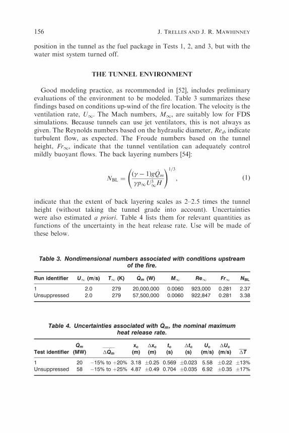
THE TUNNEL ENVIRONMENT

Good modeling practice, as recommended in [52], includes preliminaryevaluations of the environment to be modeled. Table 3 summarizes thesefindings based on conditions up-wind of the fire location. The velocity is theventilation rate, U1. The Mach numbers, M1, are suitably low for FDSsimulations. Because tunnels can use jet ventilators, this is not always asgiven. The Reynolds numbers based on the hydraulic diameter, Red, indicateturbulent flow, as expected. The Froude numbers based on the tunnelheight, Fr1, indicate that the tunnel ventilation can adequately controlmildly buoyant flows. The back layering numbers [54]:

NBL ¼� � 1ð Þg _Qm

�p1U31H

!1=3

, ð1Þ

indicate that the extent of back layering scales as 2–2.5 times the tunnelheight (without taking the tunnel grade into account). Uncertaintieswere also estimated a priori. Table 4 lists them for relevant quantities asfunctions of the uncertainty in the heat release rate. Use will be made ofthese below.

Table 3. Nondimensional numbers associated with conditions upstreamof the fire.

Run identifier U1 (m/s) T1 (K) _Qm (W) M1 Re1 Fr1 NBL

1 2.0 279 20,000,000 0.0060 923,000 0.281 2.37Unsuppressed 2.0 279 57,500,000 0.0060 922,847 0.281 3.38

Table 4. Uncertainties associated with _Qm, the nominal maximumheat release rate.

Test identifier

_Qm

(MW) � _Qm

xc

(m)�xc

(m)tc(s)

�tc(s)

Uc

(m/s)�Uc

(m/s) �T

1 20 �15% to þ20% 3.18 �0.25 0.569 �0.023 5.58 �0.22 �13%Unsuppressed 58 �15% to þ25% 4.87 �0.49 0.704 �0.035 6.92 �0.35 �17%


SIMULATIONS

CFD Model – FDS 4.0.7

FDS 4.0.7 was used for all the simulations. FDS 4 is a 3D large eddysimulation CFD model [55,56] created specifically for studies related to fireprotection engineering and fire science. It contains many sub-models andcontrol features that allow inclusion of items such as vents and nozzles,which open and close at specified times. The following subsections discusscertain aspects in more detail.

The FDS simulations were run on a cluster of Linux computers comprisedof Pentium IV single processors with 4GB of memory each and multi-coreprocessors with access to 8GB of memory. Each processor/core had a clockspeed in the 3GHz range. Run times ranged as long as 7 days.

Modifications to FDS4

Overall, the ‘official’ release of FDS 4.0.7 has been used for all thecalculations. However, it has one inadequacy that was rectified for thisstudy. FDS4 calculates the log-normal standard deviation, rLN, from theRosin-Rammler exponent, gRR, by imposing slope continuity at theintersection between the two branches of the composite distribution.Unfortunately, there is no justification for this smoothness and it hasbeen found to provide a poor prediction of the diameter at the 10%cumulative volume fraction point (Dv10) for watermist applications. Figure 3compares Rosin-Rammler/log-normal fits with measured data that wereobtained in a separate study [57,58] for a Marioff 4S 1MC8MB1100 nozzle.The smooth log-normal branch advocated by FDS4 provides a poorerrepresentation of the data than does the nonsmooth branch obtained by themethods presented in [4,52]. This was found to be the case with all of thewater mist nozzle data that the authors validated. Hence the version ofFDS4 used for the current study was modified so that both gRR and rLN

could be input and then processed as input in all the pertinent calculationswithin FDS4. Both gRR and rLN can be independently defined in FDS5.

Heat of Combustion

The gross heat of combustion of ‘wood’ burned under optimumconditions may be as high as 20.4MJ/kg [59]. However, for the currentinvestigation, a �HC of 15MJ/kg for wood in cribs was used based ona review of the available published data and the understanding that the


water mist would not allow the full 20.4MJ/kg to be achieved. This value isdeemed to be representative of ‘standard severity’ fuel packages, mainlycommon wood combustibles.

Oxygen Depletion

It is well known that one of the suppression mechanisms of water mist isoxygen depletion. The evaporating water displaces the oxygen, resulting inlower oxygen concentration. Combustion itself consumes the availableoxygen. FDS can alter the heat release rate by comparing the local oxygenconcentration and temperature with an oxygen volume fraction-temperaturemap [56] that delimits burn and no burn zones. The heat release ratereduction algorithm is invoked at cells that bind the flame interface. AsFigure 4 shows, runs performed with this oxygen depletion option turned ondid not always track the input HRR because of dips related to localsuppression of the HRR. (This effect was more pronounced in other tests

d (µm)

Cum

ulat

ive

volu

me

frac

tion

F (

d)

0

0

50

50

100

100

150

150

200

200

250

250

300

300

350

350

400

400

450

450

500

500

0.0 0.0

0.1 0.1

0.2 0.2

0.3 0.3

0.4 0.4

0.5 0.5

0.6 0.6

0.7 0.7

0.8 0.8

0.9 0.9

1.0 1.0

1.1 1.1

Rosin-Rammler branchNonsmooth log-normal branchSmooth log-normal branchMeasured

Figure 3. The nonsmooth (at the median drop size point) log-normal branch of cumulativevolume fraction for a Marioff 4S 1MC 8MB 1100 water mist nozzle better matches the data thandoes the smooth default of standard FDS4. (The color version of this figure is available online.)


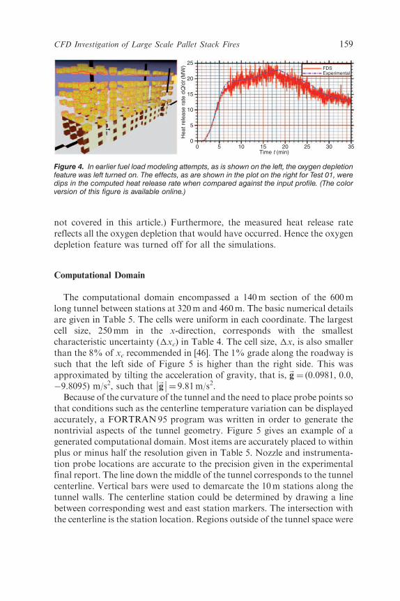
not covered in this article.) Furthermore, the measured heat release ratereflects all the oxygen depletion that would have occurred. Hence the oxygendepletion feature was turned off for all the simulations.

Computational Domain

The computational domain encompassed a 140m section of the 600mlong tunnel between stations at 320m and 460m. The basic numerical detailsare given in Table 5. The cells were uniform in each coordinate. The largestcell size, 250mm in the x-direction, corresponds with the smallestcharacteristic uncertainty (�xc) in Table 4. The cell size, �x, is also smallerthan the 8% of xc recommended in [46]. The 1% grade along the roadway issuch that the left side of Figure 5 is higher than the right side. This wasapproximated by tilting the acceleration of gravity, that is, g

!

¼ (0.0981, 0.0,�9.8095) m/s2, such that g

!�� ¼ 9.81m/s2.

Because of the curvature of the tunnel and the need to place probe points sothat conditions such as the centerline temperature variation can be displayedaccurately, a FORTRAN95 program was written in order to generate thenontrivial aspects of the tunnel geometry. Figure 5 gives an example of agenerated computational domain. Most items are accurately placed to withinplus or minus half the resolution given in Table 5. Nozzle and instrumenta-tion probe locations are accurate to the precision given in the experimentalfinal report. The line down the middle of the tunnel corresponds to the tunnelcenterline. Vertical bars were used to demarcate the 10m stations along thetunnel walls. The centerline station could be determined by drawing a linebetween corresponding west and east station markers. The intersection withthe centerline is the station location. Regions outside of the tunnel space were

25

Hea

t rel

ease

rat

e dQ

/dt (

MW

)

20

15

10

5

00 5 10 15

Time t (min)20

FDSExperimental

25 30 35

Figure 4. In earlier fuel load modeling attempts, as is shown on the left, the oxygen depletionfeature was left turned on. The effects, as are shown in the plot on the right for Test 01, weredips in the computed heat release rate when compared against the input profile. (The colorversion of this figure is available online.)


blocked off in order to avoid calculating flows in unwanted areas. Thelocation of items such as nozzles and thermocouple trees were based oncenterline station location. Points off the centerline were measured along theradius perpendicular to the centerline.

Boundary Conditions

The default thermal boundary condition was based on the properties ofconcrete as reported in Tables 6 and 7. The section of the ceiling betweenstations 370m and 420m was protected by two layers of Promat Promatect-H [60,61] insulating board. Refer to Tables 6 and 7. The right (plan north)boundary condition is open. Gases enter and leave this area according to the

Table 5. Summary of FDS 4.0.7 input parameters shared amongst thedifferent simulations.

Category Parameter Value

CFD Domain Facility San Pedro de Anes Research TunnelSimulation dimensions 140 m� 23 m� 5.17 m

Numerical Grid dimensions 560�100�24 cellsCell size 250�230�215 mmTotal # of cells 1,344,000Gravity vector (0.0981, 0.0, �9.8095) m/s2

Wall boundary conditions ConcreteFloor boundary conditions ConcreteCeiling boundary conditions Concrete/Promat Promatect-H

Nozzle Type Marioff 4S1MD6MD(1000,10RE)water mist

Configuration 4 m� 3.3 m grid, hybrid (1000,10RE)or 10RE only

Activation criteria Times as determined fromexperimental data

320

320. 355. 390. 425. 460.

330 340 350 360 370 380 390 400 410 420 430 440 450 460

Figure 5. The generic computational domain for a 140 m curved section of tunnel. The leftend of the tunnel (plan south) contains the forced flow boundary condition. The right end(plan north) is open. The water mist system is situated between stations 356 m and 424 m.The diagram shows ceiling thermocouples, four thermocouple trees, and a composite fuelload centered on station 390 m. (The color version of this figure is available online.)


difference between the local and the outside pressure heads. The left (plansouth) boundary condition is a fixed velocity according to Table 1. Becauseof the curved geometry, the velocity at each cell in the y-direction woulddiffer in its x- and y-components. Hence the left boundary was broken upinto vertical cell strips as is shown in Figure 6. The entries for the velocity atthe center of each cell strip were calculated and output using theaforementioned domain generation program. The specified velocityboundary condition has the drawback that it does not let back layeringpass through it. However, this boundary at station 320m was sufficiently faraway from the instrumented section (between 345m and 450m) so that flowreversal had little impact on the results of the simulations.

Because mechanical forces in the governing equations underlying FDSrespondwith infinite speed [52,55], the velocity boundary condition establishesitself almost immediately throughout the length of the tunnel. (FDS has adefault 1 s ramp up period for numerical stability reasons.) Nonetheless thereare other transients, such as thewake downstream of the pallet stack, that needtime to decay to the predominant turbulent flow. For this reason, up to 1minof delay time was provided before the fire was allowed to start burning.

Table 7. Thicknesses of boundary elements.

Item Thickness (m)

Tunnel concrete 0.40Ceiling slabs 0.25Floor 0.30Promat boards 0.032Gypsum board 0.013Wood 0.20Plate thermometer steel 0.0007

Table 6. Thermal properties of the thermally thick surfaces used in theFDS modeling.

Surface name

Thermalconductivityk (W/(m �K))

Density q(kg/m3)

Specific heatc (J/(kg �K)) Reference

Concrete Variable 2070 Variable [72]Gypsum board 0.48 1440 840 [73]Wood 0.17 500 2.5 [73]PT-Steel 40 7800 460 [73]Promat Promatect-H Variable 870 920 [60]


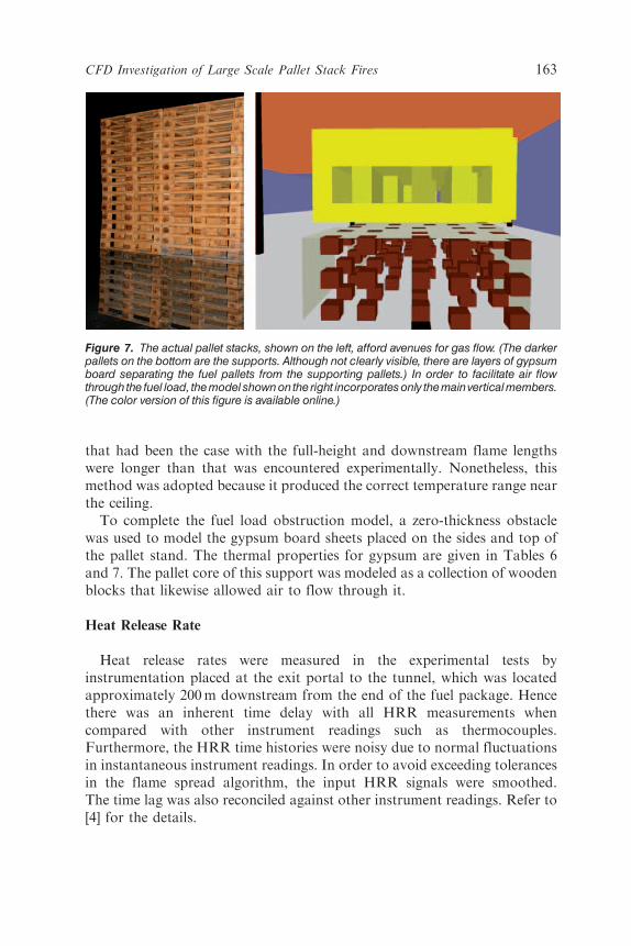
Fuel Load and Pallet Supports

Because of the nominal ¼m resolution in the computational domain, thefull detail of the stacked pallets could not be represented. Instead, methodswere explored by which some of the effects of flow through porous mediacould be obtained given that FDS has no such capabilities and given theresolution used for the simulations. In the final method adopted, denoted asthe ‘top cell method,’ the fuel load was modeled as the main member in thepallet load with wood thermal boundary conditions (see Figures 7 and 8 forvisualizations of the pallet stacks that formed the fuel array). The porosityof pallet stacks varies in the downstream direction but a uniform porosityapproach was pursued. Although the sole function of the fuel load in the topcell method is to support the top cells, modeling the fuel load as a collectionof main member allows air to flow through the arrangement. This addressedthe concern of having an otherwise impenetrable obstacle in the center of thetunnel. Initial trials with a full height commodity found that not enoughspace was available for flame volume, even with the receding pallet stack.Much better results were obtained with a half height fuel load. This methodallowed for more flame volume above the fire bed cells that are all locatedon one vertical plane. The drag across the half-height load was lower than

17.2 23.0

Figure 6. Diagram illustrating the method of inputting the upstream velocity boundarycondition as a series of vertical strips, one cell-width wide. (The color version of this figure isavailable online.)


that had been the case with the full-height and downstream flame lengthswere longer than that was encountered experimentally. Nonetheless, thismethod was adopted because it produced the correct temperature range nearthe ceiling.

To complete the fuel load obstruction model, a zero-thickness obstaclewas used to model the gypsum board sheets placed on the sides and top ofthe pallet stand. The thermal properties for gypsum are given in Tables 6and 7. The pallet core of this support was modeled as a collection of woodenblocks that likewise allowed air to flow through it.

Heat Release Rate

Heat release rates were measured in the experimental tests byinstrumentation placed at the exit portal to the tunnel, which was locatedapproximately 200m downstream from the end of the fuel package. Hencethere was an inherent time delay with all HRR measurements whencompared with other instrument readings such as thermocouples.Furthermore, the HRR time histories were noisy due to normal fluctuationsin instantaneous instrument readings. In order to avoid exceeding tolerancesin the flame spread algorithm, the input HRR signals were smoothed.The time lag was also reconciled against other instrument readings. Refer to[4] for the details.

Figure 7. The actual pallet stacks, shown on the left, afford avenues for gas flow. (The darkerpallets on the bottom are the supports. Although not clearly visible, there are layers of gypsumboard separating the fuel pallets from the supporting pallets.) In order to facilitate air flowthrough the fuel load, the model shown on the right incorporates only the main vertical members.(The color version of this figure is available online.)


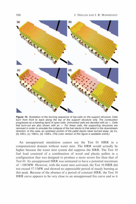
The flame spread methodology was as follows. The top cells on the topof the loads would start to burn according to the input HRR curve. Eachcell had the same heat release rate per unit area, _Q00. This quantity variedfrom simulation to simulation. It was determined by taking the maximumHRR achieved in a test and multiplying it by a scaling factor proportionalto the cell-life-to-run-time ratio, dividing it by the number of availablecells, and by the area of one top cell. In the absence of longitudinal flamespread data, each cell was given a finite life of about a quarter of the totalsimulation time (see Figure 9 for an example). This would create a de factospreading front across the surface of the fuel load. The number ofavailable top cells varied from simulation to simulation as well, beingdetermined by the fuel array dimensions and by the percentage of thepallet load that was left standing at the termination of the test (as listed inTable 2). Once a strip of top cells ceased to burn, the supporting obstacleswere removed as well. The progression was from strip center cell to cellson the left and right (in an even fashion as can be seen in Figure 10) andfrom the front (upstream) to the back (downstream) of the pallet load(again, refer to Figure 10).

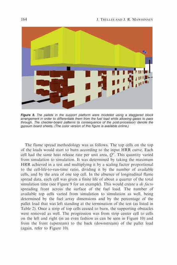
Figure 8. The pallets in the support platform were modeled using a staggered blockarrangement in order to differentiate them from the fuel load while allowing gases to passthrough. The checker-board patterns (a consequence of the post-processor) denote thegypsum board sheets. (The color version of this figure is available online.)


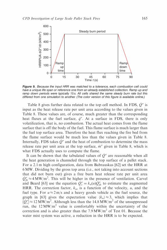
Table 8 gives further data related to the top cell method. In FDS, _Q00 isinput as the heat release rate per unit area according to the values given inTable 8. These values are, of course, much greater than the correspondingheat fluxes at the fuel surface, _q00. At a surface in FDS, there is onlyvolatilization, that is, no combustion. The actual heat comes from the flamesurface that is off the body of the fuel. This flame surface is much larger thanthe fuel top surface area. Therefore the heat flux reaching the fire bed fromthe flame surface would be much less than the values given in Table 8.Internally, FDS takes _Q00 and the heat of combustion to determine the massrelease rate per unit area at the top surface, _m00 given in Table 8, which iswhat FDS actually uses to compute the flame.

It can be shown that the tabulated values of _Q00 are reasonable when allthe heat generation is channeled through the top surface of a pallet stack.For a 2.1m high configuration, data from Babrauskas [62] set the HRR at6MW. Dividing by the gross top area (i.e., not taking into account sectionsthat did not burn out) gives a free burn heat release rate per unit area_Q00fb� 4MW/m2. This will be higher in the presence of ventilation. Carveland Beard [63] use the equation _Q00v ¼ kuðuÞ _Q00fb to estimate the augmentedHRR. The correction factor, ku, is a function of the velocity, u, and thefuel type. For u� 2m/s and a heavy goods vehicle as the fuel source, thegraph in [63] gives the expectation value kuh i� 3, which implies that

_Q00v� �� 12MW/m2. Although less than the 14.8MW/m2 of the unsuppressed

run, the 12MW/m2 value is comfortably within the uncertainty of thecorrection and is also greater than the 7.9MW/m2 of Test 01. Because thewater mist system was active, a reduction in the HRR is to be expected.

Rampdowntime

Steady burn period

Rampup

time

Time t (s)

HR

RP

UA

dQ

¥/dt

(kW

/m2)

0 15 30 45 60 75 900

100

200

300

400

500

600

Figure 9. Because the input HRR was matched to a tolerance, each combustion cell couldhave a unique life span or reference one from an already established collection. Ramp up andramp down periods were typically 15 s. All cells shared the same steady burn rate but thisdiffered from one simulation to another. (The color version of this figure is available online.)


An unsuppressed simulation cannot use the Test 01 HRR in acomputational domain without water mist. The HRR would actually behigher because the water mist system did suppress the HRR. The Test 10fuel load consisted of a combination of wood and plastic pallets in aconfiguration that was designed to produce a more severe fire than that ofTest 01. Its unsuppressed HRR was estimated to have a potential maximumof �100MW. However, with the water mist activated, the Test 10 HRR didnot exceed 57.5MW and showed no appreciable period of steady burning atthis peak. Because of the absence of a period of constant HRR, the Test 10HRR curve appears to be very close to an unsuppressed fire curve and so it

Figure 10. Illustration of the burning sequence of top-cells on the support structure. Cellsburn from front to back along the top of the support structure only. The combustionprogresses as a traveling band of open cells. Uninvolved cells are denoted with an �. Cellsthat burn-out are also shown with an �. For these cells, the supporting structures areremoved in order to simulate the collapse of the fuel stacks to that extent in the downstreamdirection. In this case, an upstream portion of the pallet stacks never burned away: (a) 0 s,(b) 430 s, (c) 1094 s, (d) 1446 s. (The color version of this figure is available online.)


was chosen to be representative of an unsuppressed fire. The fuel geometryand ventilation of Test 01 were used for the unsuppressed run. Theunsuppressed HRR could have been that of Test 01 until the nozzles cameon, switching to the Test 10 HRR from then on. However, it was decided touse the unadulterated Test 10 HRR because it came directly frommeasurements. A consequence of this decision is that the two runs start todiffer noticeably just before the water mist system comes on in Test 01.

Watermist System

Activation times for the open and thermally activated water mist nozzleswere obtained from the experimental data. The sources include notes onobservations made during the tests and the system water pressure plots.Even though the domain generation program creates the whole water mistsystem, only nozzles that activated were used in each simulation in order tominimize the calculation overhead. The pressure in the nozzle characteriza-tion files was set to match the nominal zone pressures for each test.

The default policy of FDS4 is to remove droplets that have reached the floor.The opposite setting would use the droplets that reached the ground inevaporation and heat transfer calculations. This would have the desirable effectof cooler floor temperatures but at the cost of extended run times because ofthe increasing number of droplets that FDS4 would have to manage.Simulations were performed which maintained droplets on the floor untilthey completely evaporated away. The differences in the results were negligible.Hence the simulation suite used the option to remove droplets once theyreached the floor (i.e., the lowest index in the z-coordinate computational grid).

The spherical model for characterizing the nozzle was employed. In thismethodology, droplets can be introduced through any of the user-definedsolid angles that make up the sphere surrounding the nozzle (see [52] forfurther details). The sphere was chosen to have a radius of 0.2m and wasdivided into 1056 solid angles; 54 of the solid angles were assigned a non-zero flow value. The distribution of the droplets from the 54 solid angles was

Table 8. Parameters at the fire boundary conditions( _Q00 is the heat release rate per unit area and _m00 is the mass

release rate per unit area).

Test identifier No. of cells _Q00 (kW/m2) _m00 (kg/s/m2)

1 322 7870 0.525Unsuppressed 334 14,800 0.988


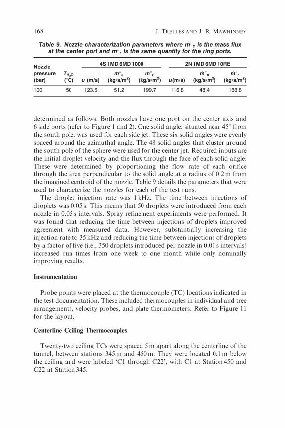
determined as follows. Both nozzles have one port on the center axis and6 side ports (refer to Figure 1 and 2). One solid angle, situated near 458 fromthe south pole, was used for each side jet. These six solid angles were evenlyspaced around the azimuthal angle. The 48 solid angles that cluster aroundthe south pole of the sphere were used for the center jet. Required inputs arethe initial droplet velocity and the flux through the face of each solid angle.These were determined by proportioning the flow rate of each orificethrough the area perpendicular to the solid angle at a radius of 0.2m fromthe imagined centroid of the nozzle. Table 9 details the parameters that wereused to characterize the nozzles for each of the test runs.

The droplet injection rate was 1 kHz. The time between injections ofdroplets was 0.05 s. This means that 50 droplets were introduced from eachnozzle in 0.05 s intervals. Spray refinement experiments were performed. Itwas found that reducing the time between injections of droplets improvedagreement with measured data. However, substantially increasing theinjection rate to 35 kHz and reducing the time between injections of dropletsby a factor of five (i.e., 350 droplets introduced per nozzle in 0.01 s intervals)increased run times from one week to one month while only nominallyimproving results.

Instrumentation

Probe points were placed at the thermocouple (TC) locations indicated inthe test documentation. These included thermocouples in individual and treearrangements, velocity probes, and plate thermometers. Refer to Figure 11for the layout.

Centerline Ceiling Thermocouples

Twenty-two ceiling TCs were spaced 5m apart along the centerline of thetunnel, between stations 345m and 450m. They were located 0.1m belowthe ceiling and were labeled ‘C1 through C22’, with C1 at Station 450 andC22 at Station 345.

Table 9. Nozzle characterization parameters where _m00c is the mass fluxat the center port and _m00r is the same quantity for the ring ports.

Nozzlepressure(bar)

TH2O

(8C)

4S 1MD 6MD 1000 2N 1MD 6MD 10RE

u (m/s)

_m00c(kg/s/m2)

_m00r(kg/s/m2) u(m/s)

_m00c(kg/s/m2)

_m00r(kg/s/m2)

100 50 123.5 51.2 199.7 116.8 48.4 188.8


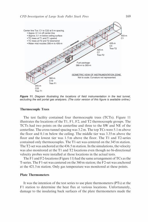
Thermocouple Trees

The test facility contained four thermocouple trees (TCTs). Figure 11illustrates the locations of the T1, F1, F2, and T2 thermocouple groups. TheTCTs had two points on the centerline and three to the SW and NE of thecenterline. The cross-tunnel spacing was 3.2m. The top TCs were 5.1m abovethe floor and 0.1m below the ceiling. The middle tier was 3.35m above thefloor and the lowest tier was 1.5m above the floor. The T1 and T2-seriescontained only thermocouples. The T1-set was centered on the 345m station.TheT2-setwas anchored at the 436.5mstation. In the simulations, the velocitywas also monitored at the T1 and T2 locations even though no bi-directionalvelocity probes were installed at those locations in the actual tests.

The F1 andF2-locations (Figure 11) had the same arrangement of TCs as theT-series. The F1-set was centered on the 360m station; the F2-set was anchoredat the 421.5m station. Only gas temperature was monitored at these points.

Plate Thermometers

It was the intention of the test series to use plate thermometers (PTs) at theF1 station to determine the heat flux at various locations. Unfortunately,damage to the insulating back surfaces of the plate thermometers made the

Center line Tcs: C1 to C22 at 5-m spacing.• Appox. 0.1-m off center-line• Approx. 0.1 m below ceiling surface• TC trees at T1 and F1 upwind• TC trees at F2 and T2 downwind• Water mist nozzles 356-m to 426-m

345-mC22Tree T1

360-mC19Tree F1

Fuel package:386-m to 393-m

420-mC7Tree F2

435-mC4Tree T2

450-mC1

ISOMETRIC VEIW OF INSTRUMENTATION ZONE Not to scale. Curvature not represented.

Figure 11. Diagram illustrating the locations of field instrumentation in the test tunnel,excluding the exit portal gas analyzers. (The color version of this figure is available online.)


measurements unreliable. Plate thermometers stabilize temperature readingsduring highly turbulent fire conditions. Hence they are useful for establishingperformance criteria for water mist systems. It was decided to insert them intheCFDanalyses. Each plate thermometer wasmodeled as a single-cell block.The data collection side had the properties of 0.7mm thick steel with aperfectly insulated backing. The plate thermometer face had the dimensions ofthe corresponding computational cell surface. This is as close as therecommendations in [64] could be followed given the limitations of resolutionand of the FDS model. The plate thermometer temperature is the walltemperature of the exposed face calculated by FDS, thus providing a physics-based model for damped temperatures. In addition, at the face of each platethermometer, the net heat flux calculated by FDS was recorded. Unlike themethodology presented in [64], where the heat fluxes were calculated fromdamped temperature readings, thenetheat flux to a surface as calculatedbyFDSis undamped. Figure 12 shows the downstream plate thermometers for Test 1.

BASIC VERIFICATIONS

Verification and validation have been performed according toDepartment of Defense Guidelines [65]. In this section, certain calculated

Figure 12. The three cubes visible behind the fuel load are the downstream platethermometers used in the Test 1 simulation. The dark face on each block indicates the platethermometer orientation. (The color version of this figure is available online.)


values from the simulations of five fire tests are verified, that is, examinedfor reasonableness, when compared to the known or measured conditionsduring the fire tests. Comparison of the calculated conditions from thesimulations, with corresponding test plots from the fire test instrumentation,is presented and discussed in the next major section.

Tunnel Ventilation Air Velocity

The ventilation air velocity in the tunnel prior to ignition of the fire wasmeasured for each test as an average over a nine-point equal area traverseupwind of the fuel array. This average was input as a boundary condition.To verify that the simulation reflected the measured ventilation conditions,the calculated average air velocity versus time plots are shown for aparticular location. The averages of the ventilation air velocities at the T1location, 40m upstream of the fire, are shown in Figure 13. For the lowerventilation velocities and faster fire growth rates, the back-layering couldreach the T1-station. This can be seen in Figure 13 as a disruption of theotherwise steady readings. Recall that the grade of the tunnel roadwayfavors buoyant flow in the direction opposite to the fan velocity. The valuefor Run 1 in Table 1 was used for the unsuppressed run (i.e., 2m/s).

The T1 locations at which measurements were made were not the ceilingpoints where the back layering was strongest. The back layering reduced thecross-sectional area through which the flow associated with tunnel ventilationcould travel. It is also affected by the fixed velocity boundary condition as

Time t (s)

Spe

ed v

(m

/s)

0 240 480 720 960 1200 1440 1680 1920 21600.5

1.0

1.5

2.0

2.5

3.0

3.5

UnsuppressedTest 01Test 02Test 03Test 10Test 13

Figure 13. Simulation results for the velocities at the T1 location as functions of time.(The color version of this figure is available online.)


mentioned above. Hence, by continuity, the measured velocity at the stationsbelow the back-layer increased as is evidenced by Figure 13. This implies that,even though the purpose of Figure 13 is basic verification of a velocityboundary condition, it also serves to indicate when significant back-layeringarrived at station T1. Because of the high heat release rate in the unsuppressedrun, the back layering reached the T1 position by 200 s and dominated thevelocity readings from thereon. Conditions before 200 s show that the targetvelocity was achieved. In spite of the limitations of the ventilation BC,Figure 13 shows no evidence of recirculated flow reaching the T1 position.

Heat Release Rates

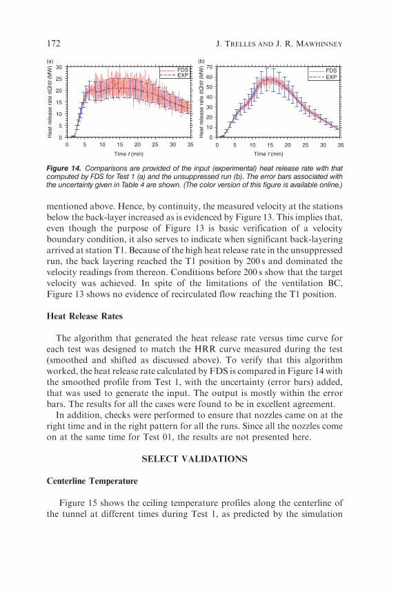
The algorithm that generated the heat release rate versus time curve foreach test was designed to match the HRR curve measured during the test(smoothed and shifted as discussed above). To verify that this algorithmworked, the heat release rate calculated by FDS is compared in Figure 14 withthe smoothed profile from Test 1, with the uncertainty (error bars) added,that was used to generate the input. The output is mostly within the errorbars. The results for all the cases were found to be in excellent agreement.

In addition, checks were performed to ensure that nozzles came on at theright time and in the right pattern for all the runs. Since all the nozzles comeon at the same time for Test 01, the results are not presented here.

SELECT VALIDATIONS

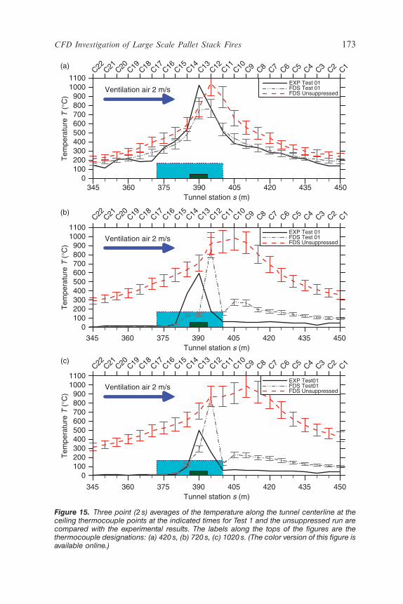
Centerline Temperature

Figure 15 shows the ceiling temperature profiles along the centerline ofthe tunnel at different times during Test 1, as predicted by the simulation

Time t (min)

Hea

t rel

ease

rat

e dQ

/dt (

MW

)

0 5 10 15 20 25 30 350

5

10

15

20

25

30(a) (b)

FDSEXP

Time t (min)

Hea

t rel

ease

rat

e dQ

/dt (

MW

)

0 5 10 15 20 25 30 350

10

20

30

40

50

60

70FDSEXP

Figure 14. Comparisons are provided of the input (experimental) heat release rate with thatcomputed by FDS for Test 1 (a) and the unsuppressed run (b). The error bars associated withthe uncertainty given in Table 4 are shown. (The color version of this figure is available online.)


Ventilation air 2 m/s

Tunnel station s (m)

Tem

pera

ture

T (

°C)

345 360 375 390 405 420 435 450

C22 C21 C20 C19 C18 C17 C16 C15 C14 C13 C12 C11 C10 C9 C8 C7 C6 C5 C4 C3 C2 C1



0100200300400500600700800900

10001100

EXP Test 01FDS Test 01FDS Unsuppressed

(a)



Tem

pera

ture

T (

°C)

345 360 375 390 405 420 435 450

0100200300400500600700800900

10001100

EXP Test 01FDS Test 01FDS Unsuppressed

(b)



Tem

pera

ture

T (

°C)

345 360 375 390 405 420 435 450

0100200300400500600700800900

10001100

EXP Test01FDS Test01FDS Unsuppressed

(c)

Figure 15. Three point (2 s) averages of the temperature along the tunnel centerline at theceiling thermocouple points at the indicated times for Test 1 and the unsuppressed run arecompared with the experimental results. The labels along the tops of the figures are thethermocouple designations: (a) 420 s, (b) 720 s, (c) 1020 s. (The color version of this figure isavailable online.)


and as measured in the fire test. The lower abscissa shows the tunnel stationnumbers and the upper abscissa shows the corresponding TC designation.The extent of the pallet array is indicated by the block above the lowerabscissa. The larger rectangle denotes the area protected by water mist.Figure 15 gives three-point (2 s) averages of the temperature at the ceiling forthree times, as predicted by the simulation for Test 1. The first time (420 s) isindicative of the highest temperature conditions just before the water mistsystem came on. Each successive time period was 5min later than theprevious one, and is cooler than the profile shown for 5 minutes earlier.

The results clearly show that the water mist eliminated back layeringupstream of station 375m. The agreement of the back layering brancheswith their experimental counter points in Figure 15 is very good. Thetemperature at C14 was higher in the tests than in the simulation. From C13to C1, though, the numerical results are generally higher than the test data,the dip at C11 is due to the presence of a nozzle just below the TC. Thus,prior to activation of the water mist system, there is extremely goodagreement between the simulation and the test data for regions 10 or moremeters from the fire location. Otherwise, the tests recorded much bettertemperature reduction along the ceiling than was predicted by the model. Itmust be noted, though, that FDS is providing dry gas temperature while thetest measurements were affected by the moist environment created by thesprays and may record a ‘wet-bulb’ temperature expected to be lower thanthe gas temperature. Another point to be noted is that the error bars shownin Figure 15 refer to the uncertainty in the simulation results only. They arenot representative of the difference between test and prediction. They are anindication of how the uncertainty in the input heat release rate manifestsitself in the temperature predictions.

Immediately over the fire itself there are several differences between thesimulation and the test results. The peak temperature measured (at C13 inthe test) was above 10008C whereas the peak temperature (at C12 in thesimulation) was approximately 750–8508C (but higher at adjacent times).The shift of peak from C13 to C12 is an artifact of the method ofcharacterizing the fuel package, and is considered to be of minorsignificance.

In the area directly above the fire, flame extensions impact directly onthe ceiling. Temperatures of 8008C or greater are deemed to represent thepresence of flame [66]. The distance from the top of the fuel package to theceiling was only 1.9 meters, while the ‘flame height’ of a 20MW fire wouldbe expected to be in the order of 10m. In the confinement of a tunnel, flameheight converts to flame length in a horizontal direction. In the test data,three thermocouples (C12, C13, and C14) showed the direct influence ofintermittent or continuous flame. As shown in Figure 16, TC C14 was about


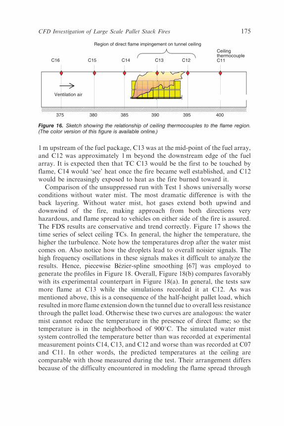
1m upstream of the fuel package, C13 was at the mid-point of the fuel array,and C12 was approximately 1m beyond the downstream edge of the fuelarray. It is expected then that TC C13 would be the first to be touched byflame, C14 would ‘see’ heat once the fire became well established, and C12would be increasingly exposed to heat as the fire burned toward it.

Comparison of the unsuppressed run with Test 1 shows universally worseconditions without water mist. The most dramatic difference is with theback layering. Without water mist, hot gases extend both upwind anddownwind of the fire, making approach from both directions veryhazardous, and flame spread to vehicles on either side of the fire is assured.The FDS results are conservative and trend correctly. Figure 17 shows thetime series of select ceiling TCs. In general, the higher the temperature, thehigher the turbulence. Note how the temperatures drop after the water mistcomes on. Also notice how the droplets lead to overall noisier signals. Thehigh frequency oscillations in these signals makes it difficult to analyze theresults. Hence, piecewise Bezier-spline smoothing [67] was employed togenerate the profiles in Figure 18. Overall, Figure 18(b) compares favorablywith its experimental counterpart in Figure 18(a). In general, the tests sawmore flame at C13 while the simulations recorded it at C12. As wasmentioned above, this is a consequence of the half-height pallet load, whichresulted inmore flame extension down the tunnel due to overall less resistancethrough the pallet load. Otherwise these two curves are analogous: the watermist cannot reduce the temperature in the presence of direct flame; so thetemperature is in the neighborhood of 9008C. The simulated water mistsystem controlled the temperature better than was recorded at experimentalmeasurement points C14, C13, and C12 and worse than was recorded at C07and C11. In other words, the predicted temperatures at the ceiling arecomparable with those measured during the test. Their arrangement differsbecause of the difficulty encountered in modeling the flame spread through

C14 C13 C12 C16 C15

Region of direct flame impingement on tunnel ceiling

004 093380 375 385 395

Ventilation air

Ceiling thermocouple C11

Figure 16. Sketch showing the relationship of ceiling thermocouples to the flame region.(The color version of this figure is available online.)


the fuel package. Peak temperatures are best judged from Figure 17 whichshows that they compare quite favorably. For the unsuppressed fire inFigure 18(c), as the fire spreads along the top of the fuel load, the temperaturebecomes more uniform along the ceiling centerline.

In examining Figure 18, it is evident that the simulation reproducedthe major cooling effects associated with the water mist acting on the fire.

Time t (min)

Tem

pera

ture

T (

°C)

0 5 10 15 20 25 30 350

100

200

300

400

500

600

700

800

900

1000

1100

C07C11C12C13C14

(a)

Time t (min)

Tem

pera

ture

T (

°C)

0 2 4 6 8 10 12 14 16 18 20 22 24 26 28 30 32 340

100

200

300

400

500

600

700

800

900

1000

1100

C07C11C12C13C14

(b)

Figure 17. Temperature histories along the tunnel centerline at the indicated instrumentationpoints for Test 1 and the unsuppressed run (a) FDS Test 01, (b) FDS Unsuppressed. (Thecolor version of this figure is available online.)


Just prior to activation of the water mist system, the temperature at TC C07,26m from the fire area, was measured at 3508C; the simulation indicated atemperature of 3008C. At the same time, TC C11 indicated temperatures justover 5008C; the simulation showed approximately 5508C. The differencesbetween test and simulation temperature were within 508C. Prior toactivation of the water mist, the thermocouples immediately above thefuel package in the flame zone, that is, C12 and C13, recorded temperatures

Time t (min)

Tem

pera

ture

T (

°C)

0 5 10 15 20 25 30 350

100200300400500600700800900

10001100

C07

C11

C12

C13

C14

(a)

Time t (min)

Tem

pera

ture

T (

°C)

0 5 10 15 20 25 30 35

0100200300400500600700800900

10001100

C07C11C12C13C14

(b)

Time t (min)

Tem

pera

ture

T (

°C)

0 2 4 6 8 10 12 14 16 18 20 22 24 26 28 30 32 34

0100200300400500600700800900

10001100

C07C11C12C13C14

(c)

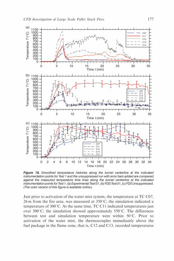
Figure 18. Smoothed temperature histories along the tunnel centerline at the indicatedinstrumentation points for Test 1 and the unsuppressed run with error bars added are comparedagainst the measured temperature time lines along the tunnel centerline at the indicatedinstrumentation points for Test 1: (a) Experimental Test 01, (b) FDS Test 01, (c) FDS Unsuppressed.(The color version of this figure is available online.)


from 8008C to 10008C. The simulation predicted temperatures in the samerange, i.e. above 8008C. Following activation of the water mist, thesimulation captured the dramatic reduction in temperatures downstream ofthe fire, particularly for the regions not immediately in the ‘flame zone’. ForTCs C10 to C07 the simulation temperatures were generally between 1508Cand 2008C, whereas the measured values indicated temperatures between508C and 1008C. Thus, the simulation temperatures were approximately1008C higher than measured values. Given that the FDS simulation reports‘gas phase’ temperature, whereas the thermocouples record a ‘wet-bulb’temperature, it is to be expected that the simulation will predict highertemperatures than measured in the area of water spray.

In the simulation, Figure 18(b) shows that only two TCs (C12 and C13)registered temperatures close to the flame temperature. It is noted that in thetest (Figure 18(a)), TC C13 was apparently in direct flame through most ofthe test, whereas TC C14 saw more heat and C12 much less than in thesimulation: the area of flame contact on the ceiling was shifted down-windto TC C12. This shift is attributed to the approximations inherent in the top-cell method. The top-cell method devised for this study succeeded inmodeling the HRR versus time curve. However, details of the geometry ofthe flames rising through the wood pallets and the transition of flame heightto flame length in the confined dimensions of the tunnel made it difficult toquantify the important parameter _Q00. Notwithstanding the shift of theregion of flame impact from C13 to C12, the simulation clearly illustratesthat there is a region directly above the fuel array where flames will impingeon the ceiling, and where it is impractical to expect temperatures to be belowthe damage threshold for concrete. The model, with reasonable accuracy,defined the limits of the area of tunnel ceiling where thermal damage tostructural concrete may be unavoidable.

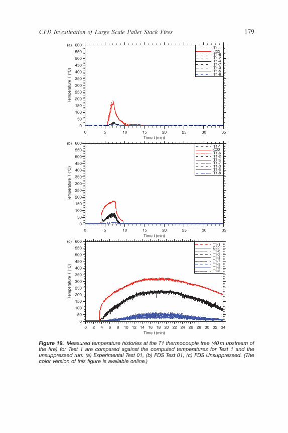
Temperature at the Thermocouple Trees

Figures 19–22 show the temperature at the thermocouple trees (TCTs) atT1, F1, F2, and T2. The arrangement of the figures is from the mostupstream TCT (T1 in Figure 19) to the most downstream TCT (T2 inFigure 21). The trees were located near enough to ceiling stations that theceiling TC reading was used for the ceiling center data. Because of thelayering, readings at the same height are presented in the same shade withdifferent line types. Typically, these cannot be discerned due to overlap ofreadings at the same level. Comparing with the experimental counterparts inFigure 19(a), the three ceiling TCs in Figure 19(b) agree very well althoughthe numerical rate of rise is steeper. The predicted mid-height temperaturesare higher than the measured values by more than 508C but the lowest rung


Time t (min)

Tem

pera

ture

T (

°C)

0 5 10 15 20 25 30 35

0

50

100

150

200

250

300

350

400

450

500

550

600T1-1C22T1-6T1-2T1-4T1-7T1-3T1-5T1-8

(a)

Time t (min)

Tem

pera

ture

T (

°C)

0 5 10 15 20 25 30 35

0

50

100

150

200

250

300

350

400

450

500

550

600T1-1C22T1-6T1-2T1-4T1-7T1-3T1-5T1-8

(b)

Time t (min)

Tem

pera

ture

T (

°C)

0 2 4 6 8 10 12 14 16 18 20 22 24 26 28 30 32 34

0

50

100

150

200

250

300

350

400

450

500

550

600T1-1C22T1-6T1-2T1-4T1-7T1-3T1-5T1-8

(c)

Figure 19. Measured temperature histories at the T1 thermocouple tree (40 m upstream ofthe fire) for Test 1 are compared against the computed temperatures for Test 1 and theunsuppressed run: (a) Experimental Test 01, (b) FDS Test 01, (c) FDS Unsuppressed. (Thecolor version of this figure is available online.)


Time t (min)

Tem

pera

ture

T (

°C)

0 5 10 15 20 25 30 35

0

50

100

150

200

250

300

350

400

450

500

550

600C19F1-6F1-4F1-7F1-3F1-5F1-8

(a)

Time t (min)

Tem

pera

ture

T (

°C)

0 5 10 15 20 25 30 35

0

50

100

150

200

250

300

350

400

450

500

550

600F1-1C19F1-6F1-2F1-4F1-7F1-3F1-5F1-8

(b)

Time t (min)

Tem

pera

ture

T (

°C)

0 2 4 6 8 10 12 14 16 18 20 22 24 26 28 30 32 34

0

50

100

150

200

250

300

350

400

450

500

550

600F1-1C19F1-6F1-2F1-4F1-7F1-3F1-5F1-8

(c)

Figure 20. Measured temperature histories at the F1 thermocouple tree (25 m upstream ofthe fire) for Test 1 are compared with the results of the simulations for Test 1 and theunsuppressed run: (a) Experimental Test 01, (b) FDS Test 01, (c) FDS Unsuppressed. (Thecolor version of this figure is available online.)


Time t (min)

Tem

pera

ture

T (

°C)

0 5 10 15 20 25 30 35

0

50

100

150

200

250

300

350

400

450

500

550

600F2-1C07F2-6F2-2F2-4F2-7F2-5F2-8

(a)

Time t (min)

Tem

pera

ture

T (

°C)

0 5 10 15 20 25 30 35

0

50

100

150

200

250

300

350

400

450

500

550

600F2-1C07F2-6F2-2F2-4F2-7F2-3F2-5F2-8

(b)

Time t (min)

Tem

pera

ture

T (

°C)

0 2 4 6 8 10 12 14 16 18 20 22 24 26 28 30 32 34

0

50

100

150

200

250

300

350

400

450

500

550

600F2-1C07F2-6F2-2F2-4F2-7F2-3F2-5F2-8

(c)

Figure 21. Measured temperature histories at the F2 thermocouple tree (27 m downstreamof the fire) for Test 1 are compared with the results of the simulations for Test 1 and theunsuppressed run: (a) Experimental Test 01, (b) FDS Test 01, (c) FDS Unsuppressed. (Thecolor version of this figure is available online.)


Time t (min)

Tem

pera

ture

T (

°C)

0 5 10 15 20 25 30 35

0

50

100

150

200

250

300

350

400

450

500

550

600T2-1C04T2-6T2-2T2-4T2-7T2-3T2-5T2-8

(a)

Time t (min)

Tem

pera

ture

T (

°C)

0 5 10 15 20 25 30 35

0

50

100

150

200

250

300

350

400

450

500

550

600T2-1C04T2-6T2-2T2-4T2-7T2-3T2-5T2-8

(b)

Time t (min)

Tem

pera

ture

T (

°C)

0 2 4 6 8 10 12 14 16 18 20 22 24 26 28 30 32 34

0

50

100

150

200

250

300

350

400

450

500

550

600T2-1C04T2-6T2-2T2-4T2-7T2-3T2-5T2-8

(c)

Figure 22. Measured temperature histories at the T2 thermocouple tree (approximately 40 mdownstream of the fire) for Test 1 (left) are compared with the results of the simulations forTest 1 and the unsuppressed run: (a) Experimental Test 01, (b) FDS Test 01, (c) FDSUnsuppressed. (The color version of this figure is available online.)


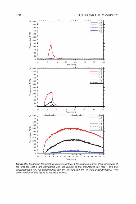
of TCs compare quite well. At F1 (Figure 20(b)), closer to the fire but stillupstream, the trend is the same. At F2 (which is downstream of the fire) inFigure 21, the agreement before water mist activation is very good. Afteractivation, the predicted ceiling TC temperatures were higher, the mid-levelTC temperature agreed very well, and the simulated lowest rung TCs wasbetter than what was measured in the tests. Overall, the comparison of thesimulation and the test results far from the fire is very good.

For Test 1, Figure 21(b) shows that, prior to activation of the water mist,the stratification in the tunnel is evident as is the case in the test data shown inFigure 21(a). Three ceiling elevation thermocouples recorded temperaturesnear 3008C. Thermocouples at 1.5 and 3.15m heights showed temperatures inthe range of 50–758C. Strikingly, the simulation also showed ceilingtemperatures at 3008C prior to system activation, only slightly highertemperatures than was measured at the 3.15m height. Temperatures at 1.5mheight were very close to those measured. After activation of the water mist inthe fire test, temperatures at all elevations and positions at F2 were measuredbetween 508C and 608C, indicating a fully mixed, non-stratified region overthe height and width of the tunnel. In contrast, the simulation indicated agreater degree of stratification at F2 than was evident in the test data. Thehigh temperature trace (TC C07 at the ceiling) at approximately 1758C wassignificantly higher than the 608C measured. However, temperatures at 1.5and 3.15m were within 108C of the measured values. As was discussed inrelation to Figure 15, FDS predicted ceiling temperatures from 508C to 1008Chigher than were measured at F2. Again, the same reasons for the differencesas were put forth in the previous section apply here as well.

Because of the lack of back layering control in the unsuppressed fire,Figure 19(c) shows that the ceiling temperature at T1 presents a burn hazardfor inhabitants at the ground. The situation only gets worse at F1(Figure 20(c)). Downstream, Figure 21(c) shows that temperatures are ashigh as 9008C at the F2 station which is 27m from the center of the fuel array.At station T2, 40m from the fire, Figure 22(c) shows moderate improvementcompared to Figure 21(c) at 27m from the fire. For the unsuppressed firecase, it is expected that even 40m away from the fire, the tunnel lining wouldbe exposed to temperatures high enough to cause spalling of unprotectedconcrete, leading to catastrophic damage to the tunnel structure.

DISCUSSION

Energy Absorbed by the Mist

A good measure of the impact of the water mist system on the fire canbe obtained by integrating the mass of water per time per area, _m00H2O

, at


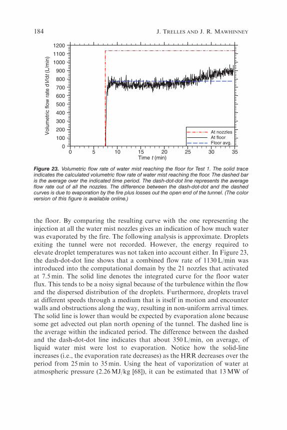
the floor. By comparing the resulting curve with the one representing theinjection at all the water mist nozzles gives an indication of how much waterwas evaporated by the fire. The following analysis is approximate. Dropletsexiting the tunnel were not recorded. However, the energy required toelevate droplet temperatures was not taken into account either. In Figure 23,the dash-dot-dot line shows that a combined flow rate of 1130L/min wasintroduced into the computational domain by the 21 nozzles that activatedat 7.5min. The solid line denotes the integrated curve for the floor waterflux. This tends to be a noisy signal because of the turbulence within the flowand the dispersed distribution of the droplets. Furthermore, droplets travelat different speeds through a medium that is itself in motion and encounterwalls and obstructions along the way, resulting in non-uniform arrival times.The solid line is lower than would be expected by evaporation alone becausesome get advected out plan north opening of the tunnel. The dashed line isthe average within the indicated period. The difference between the dashedand the dash-dot-dot line indicates that about 350L/min, on average, ofliquid water mist were lost to evaporation. Notice how the solid-lineincreases (i.e., the evaporation rate decreases) as the HRR decreases over theperiod from 25min to 35min. Using the heat of vaporization of water atatmospheric pressure (2.26MJ/kg [68]), it can be estimated that 13MW of

Time t (min)

Vol

umet

ric fl

ow r

ate

dV/d

t (L/

min

)

0 5 10 15 20 25 30 350

100

200

300

400

500

600

700

800

900

1000

1100

1200

At nozzlesAt floorFloor avg.

Figure 23. Volumetric flow rate of water mist reaching the floor for Test 1. The solid traceindicates the calculated volumetric flow rate of water mist reaching the floor. The dashed baris the average over the indicated time period. The dash-dot-dot line represents the averageflow rate out of all the nozzles. The difference between the dash-dot-dot and the dashedcurves is due to evaporation by the fire plus losses out the open end of the tunnel. (The colorversion of this figure is available online.)


energy were absorbed, on average, due to evaporation. The water depositionrate at the floor responds inversely to the HRR, indicating that moreevaporation will occur as the severity of the fire increases. This built-inresponse mechanism is one of the key fire protection features of water mistsystems.

Plate Thermometers

The plate thermometers (PT) were modeled as described above. They wereplaced at the locations of targets (4 and 5m downstream of the fire), and atTC tree stations 20m upstream and downstream of the fuel array. Figure 24shows that PT temperatures are smoother than their point-wise gastemperature counterparts. These temperatures reflect convection, radiativeexchange in the presence of smoke and water mist, the cooling effects ofdroplets, and the response of the lumped mass. Note the steep gradient inthe downstream direction. For the unsuppressed run, Figure 24(b) showsthat the temperature readings at the 4m and 5m position essentiallycoincide when the heat release rate is above 50MW.

As was mentioned above, the heat flux readings (in the units of power perunit area) are direct reflections of the thermal environment. (A positive heatflux indicates a plate surface that is heating up and a negative heat fluxcorresponds with a surface that is cooling down. The y-axis bounds inFigure 25 are burn-pain thresholds.) At about 5min, the heat fluxmeasurements at the 4 and 5m positions in Figure 25 cease their rapidgrowths due to the descent of the smoke layer. In addition, the PT readingsfor the suppressed run in Figure 25(a) are affected by the droplet streamafter the water mist system comes on. (This is a circumstance not consideredin [64].) Hence the appearance of negative heat fluxes soon after activation.From then on the heat fluxes are in response to the turbulent, smoke anddroplet seeded flows in which the plate thermometers are situated. Figure26(a) shows how the far PT heat fluxes rise until the HRR stabilizes anddrop when the water mist comes on. The upstream PT slowly cools to noheat flux. The downstream PT reading starts to drop as the smokeconcentration increases, dips negative at activation, and then registers someheat from the fire that is still burning. By the end of the run, both far PTs areregistering essentially zero heat flux. At a distance of 20m downstream ofthe pallet edge, the heat flux readings for the unsuppressed run in Figure26(b) show a rapid rise until the smoke concentration becomes heavy. Figure25(b) shows that the PT temperature is stable from about 12min to 22min.From then on it decreases. This is reflected in Figure 26(b) as negative heatfluxes (i.e., cooling of the lumped mass). For the upstream PT, after an


initial rise, Figure 26(b) shows a gradual decay in response to the decreasingvisibility associated with the unchecked back layering and to a flame frontthat is receding from the upstream PT location. A comparison of the Test 1heat fluxes with their unsuppressed counterparts clearly shows how worsethings would be even 20m away from the fire without the water mist.

Time t (min)

Tem

pera

ture

T (

°C)

0 5 10 15 20 25 30 350

50100150200250300350400450500550600650700750800850900

20 m upstream20 m downstream4 m downstream5 m downstream

(a)

Time t (min)

Tem

pera

ture

T (

°C)

0 2 4 6 8 10 12 14 16 18 20 22 24 26 28 30 32 340

50100150200250300350400450500550600650700750800850900


(b)

Figure 24. Lumped mass plate thermometer temperatures for Test 1 and the unsuppressedrun: (a) FDS Test 01, (b) FDS Unsuppressed. (The color version of this figure isavailable online.)


Comparison of Temperature Isosurfaces

Figures 27 and 28 compare the evolution of the 1008C, 3508C, 5008C, and1,0008C temperature envelopes for the suppressed and unsuppressed Test 1simulations. Figure 27 shows conditions before the water mist comes on.Both simulations have back layering to the upwind boundary of thesimulation at station 320m. They also have �40m stretches for the 3508Cand �10m stretches of the 5008C temperature envelopes. (These differbecause the HRR growths differ.) At 8min (30 s after the water mistactivated), the water mist had completely removed the back layering. At10min, the suppressed fire was near its peak. Figure 28 shows that the 1008Cenvelope is no longer in contact with the open boundary of the CFD model.By contrast, the unsuppressed simulation has a sizable pocket withtemperatures at or above 10008C. (Note that the bottom image is showinga combination of the isosurfaces and the water mist droplets.)

Time t (min)

Net

hea

t flu

x dq

¥/dt

(kW

/m2)

0 5 10 15 20 25 30 35–2.0

–1.5

–1.0

–0.5

0.0

0.5

1.0

1.5

2.0(a) (b)

20 m upstream20 m downstream

Time t (min)

Net

hea

t flu

x dq

¥/dt

(kW

/m2)

0 2 4 6 8 10 12 14 16 18 20 22 24 26 28 30 32 34–2.0

–1.5

–1.0

–0.5

0.0

0.5

1.0

1.5

2.0

20 m upstream20 m downstream

Figure 26. Net heat fluxes at the far plate thermometers: (a) Suppressed Test 01,(b) Unsuppressed Test 01. (The color version of this figure is available online.)

Time t (min)

Net

hea

t flu

x dq

¥/dt

(kW

/m2)

0 5 10 15 20 25 30 35–12–10–8–6–4–202468

1012


Time t (min)

Net

hea

t flu

x dq

¥/dt

(kW

/m2)

0 2 4 6 8 10 12 14 16 18 20 22 24 26 28 30 32 34–12–10–8–6–4–202468

1012


(a) (b)

Figure 25. Net heat fluxes at the plate thermometers: (a) Suppressed Test 01,(b) Unsuppressed Test 01. (The color version of this figure is available online.)


Floor Surface Temperature Contours

The surface floor temperature at 253 s is shown in Figure 29. This is not thetemperature of the gas but the temperature response of the concrete in thefloor to the flames above. Figure 29 shows clear evidence of shadowing inthe temperature footprint. The temperature is cool nearest to the pallet stacks.It then increases along the tunnel centerline, peaks, and then drops again.Figure 29 also shows that the highest temperatures are located off the tunnelcenterline because of the turbulence of the downstream flames.

(a) 320

320. 355. 390. 425. 460.

330 340 350 360 370 380 390 400 410 420 430 440 450 460

320330 340 350 360 370 380 390 400 410 420 430 440 450 460

(b)

320.

0:10:00.0

0:10:00.0

355. 390. 425. 460.

Figure 28. Comparison of temperature isosurfaces at 10 min. The values, from outermostenvelope to innermost, are 1008C, 3508C, 5008C, and 10008C: (a) Unsuppressed Test 1,(b) Suppressed Test 1. (The color version of this figure is available online.)

(a) 320

320. 355. 390. 425. 460.

330 340 350 360 370 380 390 400 410 420 430 440 450 460

320 330 340 350 360 370 380 390 400 410 420 430 440 450 460

(b)

320.

0:07:30.0

0:07:30.0

355. 390. 425. 460.

Figure 27. Comparison of temperature isosurfaces for the two tunnel simulations at 7.5 min(before activation of water mist in Test 1). The values, from outermost envelope to innermost,are 1008C, 3508C, 5008C, and 10008C: (a) Unsuppressed Test 1, (b) Suppressed Test 1. (Thecolor version of this figure is available online.)


CONCLUSIONS

The goal of this investigation was to increase the value of and confidencein the findings of an experimental series [2] concerned with pallet stack fires(representing very large heavy goods vehicle fires) in ventilated tunnelsprotected by water mist systems. CFD simulations were employed as theprimary means of inquiry. The CFD study required the development of aflame spread algorithm of sufficient flexibility to reasonably reproduceexperimental temperature measurements. The resulting top cell method didso while providing other necessary characteristics such as sufficient flamevolume, flow avenues through the fuel load, and sequential collapse of themodeled pallet stacks.

The CFD model was validated against data collected during the SanPedro test series. This FDS 4.0.7 model successfully predicted conditionssuch as the following:

1. Ceiling temperatures along the centerline of the tunnel prior to water mistactivation to within 508C.

2. Back layering phenomena at different ventilation air velocities before andafter activation of the water mist.

Bndrytemp

320

318

316

314

312

310

308

306

304

302

300

C

Figure 29. These contours of the floor surface temperature (at 253 s for the unsuppressed57.5 MW fire) show the phenomenon of shadowing in the lee of a burning pallet stackwhereby the region of greatest exposure is some distance away from the end of the fuel array.(The color version of this figure is available online.)


3. Conservative predictions (higher than measured in a test) of reducedceiling temperatures after water mist activation.

4. Temperatures at elevations below the ceiling at stations away from thefire.

5. The range of ceiling temperatures in the tunnel for a fire that wascontrolled by the water mist over the duration of the fire.

Issues such as the true thermocouple readings remain to be addressed. Itcan be said that the thermal management achieved by a water mist systemprovides considerable protection to inhabitants of the tunnel outside of theflame zone. Checking of back layering by the water mist system clears anavenue for emergency response teams. Propagation of fire from vehicle tovehicle along the length of the tunnel also would be unlikely. Concerns overadequate water supply are lessened because the results indicate that350L/min was sufficient to control a standard severity fire. The remainingflow provides coverage because the location of the fire cannot beanticipated. The results confirm that water mist systems are effectiveactive suppression systems for the thermal management and control of verylarge tunnel fires. When combined with fire test measurements, CFDmodeling greatly enhances the ability to analyze the performance of thesesuppression systems against very large, complex test fires.

NOMENCLATURE

c ¼ Specific heat (J/(kg �K))d ¼ Diameter (m)

Fr ¼ Froude number ()g ¼ Acceleration of gravity (9.81m/s2)k ¼ Thermal conductivity (W/(m �K))ku ¼ Ventilation correction factor ()M ¼ Mach number ()N ¼ A number ()m ¼ Mass (kg)p ¼ Pressure (Pa)Q ¼ Total heat (energy) or heat released (J)q ¼ Local heat (energy) (J)R ¼ Ideal gas constant (J/(kg �K))Re ¼ Reynolds number ()s ¼ Station along the tunnel centerline (m)T ¼ Temperature (8C)t ¼ Time (s)


U ¼ Boundary condition velocity (m/s)u ¼ Velocity (m/s)V ¼ Volume (m3)x ¼ The Cartesian position vector, equal to (x, y, z) (m,m,m)x ¼ The first Cartesian coordinate (m)y ¼ The second Cartesian coordinate (m)y ¼ A yield based on the fuel mass (kg/kg)z ¼ The third Cartesian coordinate (m)

Greekg ¼ Ratio of specific heats ()

gRR ¼ Rossin-Rammler exponent ()� ¼ The difference operator ()

�HC ¼ Heat of combustion (J/kg)� ¼ Density (kg/m3)

�LN ¼ Log-normal standard deviation ()

Superscripts— ¼ Denotes a relative uncertainty� ¼ Quantity per unit time (s�1)00 ¼ Quantity per unit area (m�2)000 ¼ Quantity per unit volume (m�3)

Subscripts0 ¼ Denotes an initial quantity

act ¼ Denotes an activated quantityBL ¼ Refers to a back layering quantityfb ¼ Denotes a free burn quantity

H2O ¼ Refers to a water quantitym ¼ Refers to a maximum quantityv ¼ Denotes a ventilated quantity1 ¼ Denotes an ambient quantity

List of Abbreviations

BFRL ¼ Building and Fire Research LaboratoryCFD ¼ Computational Fluid DynamicsHRR ¼ Heat release rateFDS ¼ Fire Dynamics Simulator

NFPA ¼ National Fire Protection AssociationNIST ¼ National Institute of Standards and Technology

Oy ¼ IncorporatedPT ¼ Plate thermometer


SFPE ¼ Society of Fire Protection EngineersTC ¼ Thermocouple

TCT ¼ Thermocouple treeUS ¼ United States

ACKNOWLEDGMENTS

Support for this research was provided by Marioff Oy and UnitedTechnologies and benefitted greatly by the guidance of Dr MaaritTuomissari, Director of Research at Marioff-UTC.

APPENDIX

To measure the HRR of very large fires as a function of time in tunnels itis necessary to capture all of the exhaust gases from the fire and direct thempast a measurement point, usually the exit portal of the tunnel. For the SanPedro de Anes tunnel tests, the quality of the data providing cross-sectionalarea, gas temperature, gas velocity, and oxygen concentration varied fromtest to test. Consequently, the uncertainty in the calculation of HRR in theexperimental work is estimated to be in the range of �15% to þ25%typically, and to range as high as 30% for two tests in which there wereproblems with an oxygen analyzer line. It is estimated that the calculation ofHRR tended to underestimate the HRR, therefore the uncertainty is notabove (þ) or below (�) the calculated value.

It is of interest to know how the relatively high uncertainty in themeasured HRR manifests itself in CFD predictions for variables of commoninterest such as temperature and velocity. As will be shown in this section,the uncertainty imparted on these variables from the heat release rate itself isnever as high as the uncertainty in the heat release rate.

The following characteristic scales for length, xc, time, tc, and velocity, Uc,are associated with a free, purely buoyant plume [52]:

xc ¼�� 1ð Þ _Qmax

�p1ffiffiffigp

" #2=5

, tc ¼�� 1ð Þ _Qmax

�p1g3

" #1=5

, Uc ¼�� 1ð Þg2 _Qmax

�p1

" #1=5

: ð2Þ

These scales are presented in terms of the highest heat release rate thatwas achieved, _Qmax, because the lowest, 0, results in trivial scales. Theremaining variables are the ratio of the specific heats, g, the ambient


pressure, p1, and the acceleration of gravity, g. Taking the differential ofeach results in the most basic expressions for the uncertainties:

�x ¼2

5

ð� � 1Þ

�p1ffiffiffigp

� �2=5� _Q

_Q3=5max

, �t ¼1

5

ð� � 1Þ

�p1g3

� �1=5� _Q

_Q4=5max

,

�U ¼1

5

ð� � 1Þg2

�p1

� �1=5� _Q

_Q4=5max

:

ð3Þ

Capital delta applied to a variable indicates its uncertainty (i.e., thestandard deviation from the calculated mean). Dividing each expression inEquation (3) by its original characteristic scale results in the relativeuncertainties:

�x ¼�x

xc¼

2

5

� _Q

_Qmax

¼2

5� _Q, �t ¼

1

5� _Q, �U ¼

1

5� _Q: ð4Þ

Temperature difference, (T�T1), whether it be in the plume, in the hotgas layer, in the ceiling jet, or from a radiative source, scales as [51]:

T� T1ð Þ / _Q2=3: ð5Þ

(Because it is independent of the heat release rate, the flame temperaturedifference scales as a constant with respect to HRR [69].) This implies thatthe relative uncertainty of the predicted temperature is

� T� T1ð Þ ¼2

3� _Q: ð6Þ

Some examples of how uncertainty in the heat release rate measurementmanifests itself in predicted variables of interest are now provided.

If � _Q ¼ 15% then �x ¼ 6%, �t ¼ 3%, �U ¼ 3%; and � T� T1ð Þ ¼ 10%:

If � _Q ¼ 20% then �x ¼ 8%, �t ¼ 4%, �U ¼ 4%, and � T� T1ð Þ ¼ 13%:




Above it was indicated that Equations (4) and (6) are the most basicexpressions for the uncertainty. This is true for a variety of reasons. First of


all, each variable depends on more than just the heat release rate. However,since the other variables in Equations (4) and (6) do not have equallyhigh uncertainties, their contributions are not expected to add much tothe overall uncertainty. Formally, the squares of the uncertainties arevariances of the respective measurements. If the sample size associatedwith the measurements was not sufficiently high then the standarddeviations would be multiplied by a bias factor which would increase theiruncertainties [70].

IfU is the relative uncertainty of any desired quantity thenU ¼UðtÞ at anymeasurement point. In other words, the uncertainty can vary with time.However, in the present analysis, U is assumed to be constant for the

duration of the test because � _Q is only estimated over the length of eachexperimental run.

The exception would be for calculated temperatures in excess of 8008C.This threshold corresponds with the continuous flame zone in theunobstructed fire plume [66] for the coldest test day (1.58C). Above 8008Cthe uncertainty does not disappear. It is just no longer possible tocharacterize it as a function of the HRR uncertainty. The temperatureuncertainty would be expected to depend on other variables but it would becontinuous across the 8008C threshold. As of this writing, no suitableexpression has been found so the policy has been adopted to keep theuncertainty constant at the 8008C value for temperatures higher than thisvalue:

� T� T1ð Þ ¼23 � _Q T� T1ð Þ if T 800�C23 � _Q 800�C� T1ð Þ if T > 800�C

(: ð7Þ

The characteristic quantities in Equation (2) formally apply to anunconstrained plume. In a tunnel, the plume and fire would be affected bythe corridor geometry and by the ventilation. However, since the plume isfundamental even in the tunnel, it is a rational starting point. Hamins andMcGrattan [51] give the example of the flame height based on the Heskestadexpression [71]. Even though flame height is a distance, because of itsdependency on heat release rate and pool fire diameter, the asymptotic

relative uncertainty of the flame height scales as �L ¼ 12 � _Q. This is greater

than the 2/5 coefficient in Equation (4). In general, the complicationsassociated with large fires with flames impinging on the graded ceiling of atunnel indicate increased uncertainty. For these reasons it is believed thatthe relative uncertainties expressed above, which were based on Equations(4) and (6), are lower bounds.


REFERENCES

1. Beard, A. and Carvel, R. (eds), The Handbook of Tunnel Fire Safety. London, ThomasTelford, 2005.

2. Mawhinney, J.R. and Ingason, H., Full-Scale Fire Testing of Suppressed Heavy GoodsVehicle Fires in Road Tunnels. Client Report HAI 5022-010-2 for Marioff Oy, Finland onthe San Pedro de Anes Test Tunnel, Hughes Associates Inc., Baltimore MD USA, 2006.

3. Ingason, H. and Lonnermark, A., ‘‘Heat Release Rates from Heavy Goods Vehicle TrailerFires in Tunnels,’’ Fire Safety Journal, Vol. 40, No. 7, 2005, pp. 648–668.

4. Mawhinney, J.R. and Trelles, J., ‘‘Testing Water Mist Systems against Large Fires inTunnels: Integrating Test Data with CFD Simulations,’’ Fire Technology, 2009; DOI:10.1007/s10694-009-0129-1 (published online).

5. Kashef, A., Benichou, N. and Lougheed, G., Numerical Modeling of Movementand Behaviour of Smoke Produced from Fires in the Ville-Marie and L.-H.-La FontaineTunnels: Literature Review. IRC-RR-141, Ottawa, Canada, National Research Council,2003.

6. Bradeis, J. and Bergmann, D.J., ‘‘A Numerical Study of Tunnel Fires,’’ Combustion Scienceand Technology, Vol. 35, 1983, pp. 133–155.

7. Kumar, S. and Cox, G., ‘‘Mathematical Modelling of Fires in Road Tunnels,’’ In: 5thInternational Symposium on Aerodynamics and Ventilation of Vehicular Tunnels, Cranfield,UK, The British Hydromechanics Research Association (BHRA), 1985.

8. Kumar, S. and Cox, G., ‘‘Radiant Heat and Surface Roughness Effects in the NumericalModelling of Tunnel Fires,’’ In: 6th International Symposium on Aerodynamics andVentilation of Vehicular Tunnels. Cranfield, UK, The British Hydromechanics ResearchAssociation (BHRA), 1988.

9. Kawabata, N., Ohashi, H. and Kato, Y., ‘‘Numerical Simulation of Fire PlumePropagation Along the Ceiling of a Down-Grade Tunnel,’’ In: Proceedings of theInternational Symposium on Aerodynamics and Ventilation of Vehicle Tunnels, London, pp.319–335, 1991.

10. Fletcher, D.F., Kent, J.H., Apte, V.B. and Green, A.R., ‘‘Numerical Simulations of SmokeMovement from a Pool Fire in a Ventilated Tunnel,’’ Fire Safety Journal, Vol. 23, No. 3,1994, pp. 305–325.

11. Rhodes, N., ‘‘Review of Tunnel Fire and Smoke Simulations,’’ In: 8th InternationalSymposium on Aerodynamics and Ventilation of Vehicular Tunnels, The BritishHydromechanics Research (BHR) Group Conference Series Publication No. 12,London, pp. 471–486, 1994.

12. Biollay, H. and Chasse, P., ‘‘Validating and Optimizing 2D and 3D Computer Simulationsfor the Ofenegg Tunnel Fire Tests,’’ In: 8th International Symposium on Aerodynamics andVentilation of Vehicular Tunnels, The British Hydromechanics Research (BHR) GroupConference Series Publication No. 12, London, pp. 357–381, 1994.

13. Bettelini, M., CFD for Tunnel Safety. Fluent User’s Meeting, Hanover, NH USA, Fluent,2001.

14. Chasse, P., Validation du code Flow3D sur un Essai Incendie du Tunnel de l’Ofenegg. Lyons,France, Centre D’etudes de Tunnels, 1995.

15. Biollay, H., ‘‘Projet Eureka 499: Simulations numeriques de l’essai d’heptane H32,’’ In:Journee de presentation de resultats de recherche a l’Arche de la defence, Paris, France, pp.1–13, 1996.

16. Woodburn, P.J. and Britter, R.E., ‘‘CFD Simulations of a Tunnel Fire – Part I,’’ FireSafety Journal, Vol. 26, No. 1, 1996, pp. 35–62.

17. Woodburn, P.J. and Britter, R.E., ‘‘CFD Simulations of a Tunnel Fire – Part II,’’ FireSafety Journal, Vol. 26, No. 1, 1996, pp. 63–90.


18. Atkinson, G.T., Bettis, R.J., Jagger, S.F. and Lea, C.J., ‘‘Fire Tests and CFD Modeling ofCritical Velocity Behavior,’’ In: ITC Seminar on Smoke and Critical Velocity in Tunnels,London, Health and Safety Laboratory, 1996.

19. Rhodes, N., ‘‘Smoke Modeling & Critical Velocity in Tunnels,’’ In: ITC Seminar on Smokeand Critical Velocity in Tunnels, London, Health and Safety Laboratory, 1996.

20. Hwang, C.C. and Edwards, J.C., ‘‘CFD Modeling of Smoke Reversal,’’ In: Proceedings ofthe International Conference on Engineered Fire Protection Design, Bethesda, MD USA,Society of Fire Protection Engineers, pp. 376–387, 2001.

21. Hwang, C.C. and Edwards, J.C., ‘‘The Critical Ventilation Velocity in Tunnel Fires—AComputer Simulation,’’ Fire Safety Journal, Vol. 40, No. 3, 2005, pp. 213–244.

22. Schabacker, J., Bettelini, M. and Rudin, Ch., ‘‘CFD Study of Temperature and SmokeDistribution in a Railway Tunnel with Natural Ventilation System,’’ Tunnel ManagementInternational, Vol. 5, No. 3, 2002, pp. 1–10.

23. SantolariaMorros, C., Ballesteros Tajadura, R., BlancoMarigorta, E. andMartinez Viejo, J.,‘‘Influencia de la Pendiente en la Ventilation Semitransversal de unTunelUrbano,’’ In: CapoteAbreu, J.A., ed., Computational Simulation Models in Fire Engineering and Research, pp. 59–68. Santander, Spain, GIDAI, 2004.

24. IRI & PBI, SOLVENT Version 1.0. Innovative Research, Inc.,/Parsons Brinkerhoff, Inc.,Minneapolis, MN USA, 2000.

25. Massachusetts Highway Department & FHA, Memorial Tunnel Fire Test VentilationProgram – Phase IV Report. Central Artery/Tunnel Project, Boston, Commonwealth ofMassachusetts, 1999.

26. Innovative Research, Reference Manual for COMPACT-3D. Innovative Research, Inc.,Minneapolis, MN USA, 1998

27. Kashef, A., Benichou, N. and Lougheed, G., Application of CFD Technique to ModelAerodynamic Tests in Road Tunnels. Ottawa, Canada, NRCC-46727, National ResearchCouncil, 2003.

28. Kashef, A., Benichou, N., Lougheed, G. and Debs, A., Numerical Modeling of AirMovement in Road Tunnels. Ottawa, Canada, NRCC-43714, National Research Council,2003.

29. Kashef, A., Benichou, N., Lougheed, G. and Debs, A., Compuational Fluid DynamicsSimulations of In-Situ Fire Tests in Road Tunnels. Ottawa, Canada, NRCC-45174, NationalResearch Council, 2004.

30. Kashef, A., Benichou, N., Lougheed, G. and Debs, A., CFD Simulations of In-Situ AirflowMeasurements in Road Tunnels. Ottawa, Canada, NRCC-47707, National ResearchCouncil, 2004.

31. Kashef, A., Benichou, N., Lougheed, G. and Debs, A., Application of CFD Techniques forModelling Fire Tests in Road Tunnels. Ottawa, Canada, NRCC-46772, National ResearchCouncil, 2004.

32. Kumar, S., ‘‘Recent Achievements in Modelling the Transport of Smoke and Toxic Gasesin Tunnel Fires,’’ In: First International Symposium on Safe & Reliable Tunnels, Lausanne,Switzerland, ITA-AITES, pp. 97–105, 2004.

33. Gant, S.E., CFD Modelling of Water Spray Barriers. HSL/2006/79. Buxton Derbyshire,UK, Health & Safety Laboratory, 2006.

34. Hart, R.A., Ren, T.X. and Edwards, J.S., ‘‘Numerical Simulation of Water MistSuppression of Tunnel-Fire Scenarios,’’ In: Third International Conference on CFD in theMinerals and Process Industries, Melbourne, Australia, CSIRO, 2003.

35. Aprili, P., Giuseppe, D., Dino, F., Zappellini, G. and Ferrari, A., ‘‘CFD Simulations of aTruck Fire in the Underground Gran Sasso National Laboratory,’’ In: Proceedings of the5th Italian Conference on Chemical and Process Engineering, Associazione Italiana DiIngegneria Chimica (AIDIC), London, Elsevier, 2002.


36. Aprili, P. and Franciotti, D., ‘‘CFD Simulations to Better Evaluate TechnicalImprovements to Reduce Fire Damage,’’ In: Bedford, T. and van Gelder, P.H.A.J.M.,eds, In: Safety and Reliability: Proceedings of ESREL 2003, European Safety and ReliabilityConference. Vol. 1, pp. 45–53. Washington, DC, Taylor & Francis, 2003.

37. McGrattan, K.B. and Hamins, A., Numerical Simulation of the Howard Street Tunnel Fire,Baltimore, Maryland, July 2001. NISTIR 6902, NUREG/CR-6793, NRC Job Code J5414,Gaithersburg, MD USA, National Institute of Standards and Technology, 2003.

38. McGrattan, K.B. and Hamins, A., ‘‘Numerical Simulation of the Howard Street TunnelFire,’’ Fire Technology, Vol. 42, No. 4, 2006, pp. 273–281.

39. van de Leur, P.H.E., Tunnel Fire Simulations for the Ministry of Public Works (in Dutch).Report B-91-0043, Delft, TNO, 1991.

40. Johansson, M., Mowrer, F.M. and de Joseph, J., ‘‘An Analysis of Conditions Resultingfrom Fire during Tunnel Boring Operations,’’ In: Interflam 2004, London, InterscienceCommunications, pp. 1505–1516, 2004.

41. McGrattan, K.B., Numerical Simulation of the Caldecott Tunnel Fire, April 1982. NISTIR7231, Gaithersburg, MD USA, National Institute of Standards and Technology, 2005.

42. Carvel, R.O. and Torero, J.L., ‘‘Refurbished Clyde Tunnel Fire Scenario: CFD Modellingand Heat Transfer Calculations,’’ Tunnel Management International, Vol. 9, No. 3–4, 2006,pp. 41–46.

43. Cafaro, E., Cima, C., Stantero, L. and Arelli, A., ‘‘Tunnel Fire Mitigation System: FullScale Tests,’’ Tunnel Management International, Vol. 9, No. 3–4, 2006, pp. 8–16.

44. Cafaro, E., Focaracci, A., Guarascio, M. and Stantero, L., ‘‘Quantitative Risk Analysis forTunnel Safety,’’ Tunnel Management International, Vol. 9, No. 3–4, 2006, pp. 32–40.

45. Hu, L.H., Huo, R. and Wang, H.B., ‘‘Experimental and Numerical Studies onLongitudinal Smoke Temperature Distribution Upstream and Downstream from theFire in a Road Tunnel,’’ Journal of Fire Sciences, Vol. 25, No. 3, 2007, pp. 23–43.

46. Kim, E., Woycheese, J. and Dembsey, N., ‘‘Fire Dynamics Simulator (Version 4.0)Simulation for Tunnel Fire Scenarios with Forced, Transient, Longitudinal VentilationFlows,’’ Fire Technology, Vol. 44, No. 2, 2008, pp. 137–166.

47. Cheong, M., Spearpoint, M. and Fleischmann, C., ‘‘Calibrating an FDS Simulation ofGoods Vehicle Fire Growth in a Tunnel Using the Runehamar Experiment,’’ Journal ofFire Protection Engineering, Vol. 19, No. 3, 2009, pp. 177–196.

48. Nmira, F., Consalvi, J., Kaiss, A., Fernandez-Pello, A. and Porterie, B., ‘‘A NumericalStudy of Water Mist Mitigation of Tunnel Fires,’’ Fire Safety Journal, Vol. 44, No. 2, 2009,pp. 198–211.

49. Chasse, P., ‘‘Sensitivity Study of Different Modeling Techniques for the ComputerSimulation of Tunnel Fires,’’ In: CFD International Users Conference, London, AEATechnology, 1993.

50. Tuovinen, H., Holmstedt, G. and Bengtson, S., ‘‘Sensitivity Calculations of Tunnel FiresUsing CFD,’’ Fire Technology, Vol. 32, No. 2, 1996, pp. 99–119.

51. Hamins, A. and McGrattan, K.B., Verification and Validation of Selected Fire Models forNuclear Power Plant Applications, Volume 2: Experimental Uncertainty. NUREG-1824 andEPRI 1011999, Rockville, MD, U.S. Nuclear Regulatory Commission and Palo Alto, CA,Electric Power Research Institute (EPRI), 2007.

52. Trelles, J. and Floyd, J.E., ‘‘Chapter 11: The Implementation and Application of aFire CFD Model,’’ In: Faghri, M. and Sunden, B., eds., Transport Phenomena in Fires,pp. 407–440. Southampton, UK, WIT Press, 2008.

53. Chan, T.S., ‘‘Measurements of Water Density and Drop Size Distributions of SelectedESFR Sprinklers,’’ Journal Fire Protection Engineering, Vol. 6, No. 2, 1994, pp. 79–87.

54. Ingason, H., ‘‘Fire Dynamics,’’ In: Beard, A. and Carvel, R., eds., The Handbook of TunnelFire Safety, pp. 231–266. London, Thomas Telford, 2005.


55. McGrattan, K.B., Fire Dynamics Simulator (Version 4) – Technical Reference Guide. NISTSpecial Publication 1018, Gaithersburg, MD USA, National Institute of Standards andTechnology, 2006.

56. McGrattan, K.B. and Forney, G.P., Fire Dynamics Simulator (Version 4) – User’s Guide.NIST Special Publication 1019, Gaithersburg, MD USA, National Institute of Standardsand Technology, 2004.

57. Mawhinney, J., DiNenno, P.J. and Williams, F.W., Water Mist Flashover Suppression andBoundary Cooling System for Integration with DC-ARM – Volume I: Summary of Testing.Technical Report NRL/MR/6180—99-8400, Washington, DC, Naval ResearchLaboratory, 1999.

58. Mawhinney, J., DiNenno, P.J. and Williams, F.W., Water Mist Flashover Suppression andBoundary Cooling System for Integration with DC-ARM – Volume II: Mist Concentrationand Fire Test Data. Technical Report NRL/MR/6180—99-8401, Washington, DC, NavalResearch Laboratory, 1999.

59. Cox, G. and Kumar, S., ‘‘Modeling Enclosure Fires Using CFD,’’ In: DiNenno, P.J.,Drysdale, D., Beyler, C.L., Walton, W.D., Custer, R.L.P., Hall Jr, J.R. and Watts Jr, J.M.,eds, SFPE Handbook of Fire Protection Engineering, 3rd edn., pp. 3-194–3-218. Quincy,MA USA, Society of Fire Protection Engineers, 2002.

60. Promat, Technical Data Sheet for Promatect-H. Genova, Italy, Promat S.p.A., 2004.

61. Promat, Promat Passive Fire Protection in Tunnels. Marketing Brochure, Ratingen,Germany, Promat GmbH, 2001.

62. Babrauskas, V., ‘‘Heat Release Rates,’’ In: DiNenno, P.J., Drysdale, D., Beyler, C.L.,Walton, W.D., Custer, R.L.P., Hall Jr, J.R. and Watts Jr, J.M., eds, SFPE Handbook ofFire Protection Engineering, 3rd edn., pp. 3-1–3-37. Quincy, MA USA, Society of FireProtection Engineers, 2002.

63. Carvel, R. and Beard, A., ‘‘The Influence of Tunnel Ventilation on Fire Behavior,’’ In:Beard, A. and Carvel, R., eds, The Handbook of Tunnel Fire Safety, pp. 184–198. London,Thomas Telford, 2005.

64. Ingason, H. and Wickstrom, U., ‘‘Measuring Incident Radiant Heat Flux Using the PlateThermometer,’’ Fire Safety Journal, Vol. 42, 2007, pp. 161–166.

65. DDR&E, Department of Defense Verification, Validation and Accreditation (VV&A)Recommended Practice Guide. Office of the Director of Defense Research and Engineering,Washington, DC, 1996.

66. Trelles, J. and Pagni, P.J., ‘‘Fire-Induced Winds in the 20 October 1991 Oakland HillsFire,’’ In: Fire Safety Science: Proceedings of the Fifth International Symposium, London,Elsevier, pp. 911–922, 1997.

67. Williams, T. and Kelley, C., gnuplot: An Interactive Plotting Program. Free SoftwareFoundation, Boston, 2004.

68. Moran, M.J. and Shapiro, H.N., Fundamentals of Engineering Thermodynamics.New York, John Wiley & Sons, 1988.

69. Quintiere, J.G., ‘‘Scaling Applications in Fire Research,’’ Fire Safety Journal, Vol. 15, No.1, 1989, pp. 3–29.

70. Figliola, R.S. and Beasley, D.E., Theory and Design for Mechanical Measurement, 2nd edn,New York, John Wiley & Sons, Inc., 1995.

71. Heskestad, G., ‘‘Fire Plumes, Flame Height, and Air Entrainment,’’ In: DiNenno, P.J.,Drysdale, D., Beyler, C.L., Walton, W.D., Custer, R.L.P., Hall Jr, J.R. and Watts Jr, J.M.,eds, SFPE Handbook of Fire Protection Engineering, 3rd edn, pp. 2-1–2-17. Quincy, MAUSA, Society of Fire Protection Engineers, 2002.

72. Harmathy, T.Z., Properties of Building Materials at Elevated Temperatures. DBR PaperNo. 1080, Ottawa, Canada, National Research Council, 1983.

73. Quintiere, J.G., Principles of Fire Behavior. Albany, NY USA, Delmar Publishers, 1998.


CFD Investigation of Large Scale Pallet Stack Fires in ...c.ymcdn.com/sites/ · PDF fileCFD...

Documents

Transcript of CFD Investigation of Large Scale Pallet Stack Fires in ...c.ymcdn.com/sites/ · PDF fileCFD...