Qing Wu1

Centre for Railway Engineering,

Central Queensland University,

Rockhampton QLD4701, Australia

e-mail: q.wu@cqu.edu.au

Colin ColeCentre for Railway Engineering,

Central Queensland University,

Rockhampton QLD4701, Australia

Maksym SpiryaginCentre for Railway Engineering,

Central Queensland University,

Rockhampton QLD4701, Australia

Yucang WangSchool of Engineering and Technology,

Central Queensland University,

Rockhampton QLD4701, Australia

Weihua MaState Key Laboratory of Traction Power,

Southwest Jiaotong University,

Chengdu 610031, China

Chongfeng WeiDepartment of Systems Design Engineering,

University of Waterloo,

Waterloo, ON N2L 3G1, Canada

Railway Air Brake Model andParallel Computing SchemeThis paper developed a detailed fluid dynamics model and a parallel computing schemefor air brake systems on long freight trains. The model consists of subsystem models forpipes, locomotive brake valves, and wagon brake valves. A new efficient hose connectionboundary condition that considers pressure loss across the connection was developed.Simulations with 150 sets of wagon brake systems were conducted and validated againstexperimental data; the simulated results and measured results reached an agreementwith the maximum difference of 15%; all important air brake system features were wellsimulated. Computing time was compared for simulations with and without parallel com-puting. The computing time for the conventional sequential computing scheme was about6.7 times slower than real-time. Parallel computing using four computing coresdecreased the computing time by 70%. Real-time simulations were achieved by parallelcomputing using eight computer cores. [DOI: 10.1115/1.4036421]

Keywords: air brake, gas dynamics, method of characteristics, railway train dynamics,parallel computing

1 Introduction

Brake is a critical aspect of railway train operations. Railwaybrake systems [1] are mainly of the air brake type which relies onpressurized air to push brake shoes or pads against wheel treads orbrake disks. This paper focuses on conventional automatic (fail-safe) air brake systems on long freight trains; electronically con-trolled pneumatic (ECP) brake systems [2] and other alternativebrake systems [1] are not discussed. Comparatively, the automaticair brake systems on long freight trains pose greater challenges formodeling and simulations in the sense of complicated fluiddynamics modeling and intensive computing loads. The modelingapproach presented in this paper can also be used to model pas-senger train air brake systems; it can also be modified to simulateECP brake systems.

Numerical modeling and simulations are indispensableapproaches to study and improve air brake systems. A reviewregarding air brake modeling prior to the 1990s can be found inRef. [3]. Another more recent review [4] regarding longitudinaltrain dynamics has classified air brake models into empirical mod-els, fluid dynamics models, and empirical–fluid dynamics models.Empirical models [5–8] use mathematical equations to fit meas-ured characteristics of air brake systems. These empirical modelsdo not necessarily follow fluid dynamics principles behind themeasured characteristics. In comparison, fluid dynamics models[9–15] describe air flows according to fluid dynamics principles.The flows described include flows in brake pipes and thosebetween various components of brake valves. Empirical–fluiddynamics models [16,17] blend the fluid dynamics models and

empirical models by retaining fluid dynamics pipe models butmodeling brake valves using empirical functions.

Fluid dynamics air brake models are clearly the most advancedamong all three types of models. However, they do have a well-known but not widely discussed disadvantage: low computingspeed. The authors’ experience with both empirical and fluiddynamics models indicates that, with the same step-size, the com-puting speed of an empirical model can be 100 times faster than afluid dynamics model. It is difficult to achieve real-time simula-tions using fluid dynamics models for long heavy haul trains (e.g.,241 vehicles) due to the large number of equations to solve. Thecomputational efficiency issue of fluid dynamics models is also animportant reason why empirical models are still commonly used[6–8]. Empirical–fluid dynamics models [16,17] can evidentlyimprove the computing speed but they also inherit some limita-tions of the empirical models. For example, the empirical valvemodels only cover the specific measured valve types and workingconditions used to develop such models.

This paper develops a detailed fluid dynamics air brake modelfor long heavy haul trains. The model includes subsystem modelsfor pipes, locomotive brake valves, and wagon brake valves.Experimental data are presented for validation. The novelty ofthis study is also contributed by the parallel computing schemethat significantly improves the computing speed of the fluiddynamics model. Computing time is compared for simulationswith and without parallel computing. A new hose connectionboundary condition is developed to consider air pressure losswhile crossing the hose connection; a pipe tee boundary conditionis improved to also consider air pressure loss.

2 Automatic Air Brake

The automatic air brake studied in this paper is illustrated asFig. 1. It consists of one (or more for distributed power trains)

1Corresponding author.Contributed by the Design Engineering Division of ASME for publication in the

JOURNAL OF COMPUTATIONAL AND NONLINEAR DYNAMICS. Manuscript received February8, 2017; final manuscript received March 28, 2017; published online May 15, 2017.Assoc. Editor: Paramsothy Jayakumar.

Journal of Computational and Nonlinear Dynamics SEPTEMBER 2017, Vol. 12 / 051017-1Copyright VC 2017 by ASME

Downloaded From: http://computationalnonlinear.asmedigitalcollection.asme.org/ on 09/08/2018 Terms of Use: http://www.asme.org/about-asme/terms-of-use

locomotive brake system and a number of wagon brake systems(one system per wagon). All systems are connected by hoseswhich allow intervehicle movements. Brake application andrelease signals are transmitted via the pressurized air in the brakepipe.

2.1 Locomotive Brake System. The locomotive brake sys-tem is shown as Fig. 2. Note that this figure shows only the trainautomatic brake parts; locomotive independent brakes that arespecifically used for locomotives are not discussed in this paper.In this system, the air compressor detects the pressure of the mainreservoir and automatically starts or stops the feed of pressurizedair to the main reservoir as required to maintain pressure. The reg-ulating valve controls the openings of /5 and /3 according to theposition of the driver’s handle and the pressure in the equalizingreservoir. The equalizing reservoir has a small volume (15 L) andacts as a pilot for the pressure change of the brake pipe. The relayvalve detects the pressure difference between the equalizing reser-voir and the brake pipe so as to change the openings of /2 and /4.When the equalizing reservoir pressure is higher than the pipepressure, /2 is opened and the main reservoir charges the brakepipe until an equilibrium is reached between the equalizing reser-voir and the brake pipe. When the pressure difference is other-wise, /4 is opened and the brake pipe discharges to atmosphereuntil an equilibrium is reached.

2.2 Wagon Brake System. The wagon brake system utilizesthe well-known principle of a “triple valve” [1]: brakes areapplied when brake pipe pressure is lower than auxiliary reservoirpressure, while brakes are released when the pressure difference isotherwise. These basic actions are achieved via the sliding valveand graduating valve as shown in Fig. 3. The service pistondivides the volume of a distributor into an upper chamber and alower chamber which are, respectively, connected to brake pipeand auxiliary reservoir. The service piston changes the positionsof the graduating valve and the sliding valve according to differ-ent pressure situations in the upper and lower chambers. There arevarious ports, orifices, and connecting grooves in the graduatingvalve, sliding valve, and sliding valve seat. Therefore, differentpositions of valves can form different air passages.

The studied wagon brake system (see Fig. 4) has the followingfeatures: quick service (two stages), braking, lapping, quickrelease, release, regulated recharge, and emergency braking (twostages). Note that in Fig. 4, /7, /11, and /16 are uncontrolledopenings (orifices or chokes); all other openings are controlled byvarious valves.

Quick service (stage 1 or preliminary): The graduating valveand the sliding valve uncover port /15. The quick service bulb hasa small volume (0.6 L) and is opened to the atmosphere via achoke /16. Therefore, a small amount of pressurized air can bevented from the brake pipe to atmosphere via the upper chamberof the distributor. The quick service feature quickly decreases thebrake pipe pressure so as to accelerate the braking process in thewagon brake system; it also accelerates the brake propagation ratein the brake pipe. Note that the pipe pressure reduction during thisstage is small (about 10 kPa).

Quick service (stage 2): The graduating valve and the slidingvalve close port /15. The second stage of quick service isachieved via the quick service limiting valve (or in-shot valve)which detects the pressure of the brake cylinder. When the cylin-der pressure is lower than a certain value (60 kPa), the valve keepsport /9 open and allows pressurized air flows into the brake cylin-der from the brake pipe via the upper chamber. The second stageof quick service has the same functions as the first stage; in addi-tion, it helps increase the cylinder pressure (in-shot) to help withextending the push rod.

Braking: The braking process occurs simultaneously with thesecond stage of quick service. During braking, the graduatingvalve and the sliding valve uncover /12 which allows pressurizedair flows from the auxiliary reservoir to the brake cylinder via thelower chamber.

Lapping: When the pressure difference between the upperchamber and the lower chamber is not enough to hold the graduat-ing valve in its up position, the graduating valve will drop andclose port /12 which stops the pressure increase in the brake cylin-der. Note that the sliding valve is not moving during lapping;therefore, brake release is not activated.

Quick release: When brake release is activated, the pressurizedair in the brake cylinder will be exhausted to the atmosphere.When the quick release valve has detected a certain rate of outflow from the brake cylinder, the quick release valve can open thecheck valve /8 which allows pressurized air that is stored in thequick release reservoir to be charged to the brake pipe via theupper chamber. The quick release feature accelerates the releaseprocess in the wagon brake system; it also increases the propaga-tion rate of brake release in the brake pipe.

Release: The graduating valve and the sliding valve close port/12 and uncover port /13. The pressurized air in the brake cylin-der is exhausted to the atmosphere. Note that the release cannotbe lapped, which means graduated release is not an option for thiswagon brake system. During the brake release, ports /10, /11, and/17 are also opened; therefore, the auxiliary reservoir and thequick release reservoir can be charged to operating pressure(500 kPa or 600 kPa) and be prepared for future actions. Port /14

can also be opened if there was any pressure loss in the emergencybulb during the brake application.

Fig. 1 Automatic air brake

Fig. 2 Locomotive brake system

051017-2 / Vol. 12, SEPTEMBER 2017 Transactions of the ASME

Downloaded From: http://computationalnonlinear.asmedigitalcollection.asme.org/ on 09/08/2018 Terms of Use: http://www.asme.org/about-asme/terms-of-use

Regulated recharge: During a release process, when the upperchamber pressure is significantly higher than that of the lowerchamber, the cage will be pushed by the sliding valve and thereturn spring will be deflected. The sliding valve will thendecrease the opening size of port /11 so as to decrease therecharging rate of the auxiliary reservoir. This feature slows therecharging of auxiliary reservoirs toward the front of the train dur-ing brake release processes, which can help to achieve a uniformrecharging rate and brake release along the train.

Emergency braking (stage 1): When the emergency valvedetects significant pressure difference between the emergencybulb and upper chamber, the emergency valve can open the checkvalve /6 which exhausts the pressurized air in the brake pipe tothe atmosphere via the upper chamber. During the emergencybraking, auxiliary reservoir, lower chamber, and brake cylinderhave the same air passages as those during the braking processthat has been described previously. The first stage of emergencybraking is very quick and drastic; it can increase brake cylinderpressure from 0 to 160 kPa in about 2 s. The fast increase of pres-sure is limited to about 160 kPa then a slower response in stage 2initiates.

Emergency braking (stage 2): As the first stage of emergencybraking is quick and drastic, it is not desirable from the traindynamics point of view to keep applying brakes at this rate. Forthis reason, the wagon brake system has a dual-stage emergency

braking feature which decreases the opening size of /13 (indi-rectly) when the cylinder pressure has reached 160 kPa. This fea-ture is designed and tuned to make sure that the train hassufficient braking capability and acceptable train dynamicsperformance during emergency braking.

3 Pipe Modeling

Pipes that were modeled (with the consideration of air flows)for each wagon include two sections of brake pipe and one sectionof branch pipe (see Fig. 4). The modeling implies conservationlaws and various boundary conditions. Hose connections weremodeled as boundary conditions. Pipes that connect the quickrelease reservoir, auxiliary reservoir, and brake cylinder were sim-plified as additional volumes [13].

3.1 Conservation Laws. The pipe model is based on a gasdynamics model developed by Benson et al. [18] for the purposeof internal combustion engine simulations. The model is illus-trated as Fig. 5 while the governing equations are expressed as[18]

@q@tþ q

@u

@xþ u

@q@xþ qu

F

dF

dx¼ 0 (1)

Fig. 3 Sliding valve and graduating valve positions: (a) release, (b) preliminary quick service, (c) brake, and (d) lapping

Fig. 4 Wagon brake system

Journal of Computational and Nonlinear Dynamics SEPTEMBER 2017, Vol. 12 / 051017-3

Downloaded From: http://computationalnonlinear.asmedigitalcollection.asme.org/ on 09/08/2018 Terms of Use: http://www.asme.org/about-asme/terms-of-use

@u

@tþ u

@u

@xþ 1

q@P

@xþ f

u2

2

u

juj4

D¼ 0 (2)

@P

@tþ u

@P

@x� a2 @q

@tþ u

@q@x

� �� k � 1ð Þq qþ uf

u2

2

u

juj4

D

!¼ 0

(3)

where q is the air density, t is the time, u is the air flow velocity, xis the position along the pipe, F is the cross-sectional area of thepipe, f is the coefficient of friction, D is the pipe diameter, P isthe air pressure, a is the speed of sound, q is the heat exchangerate, and k is the specific heat ratio. It can be seen that the modelis a one-dimensional unsteady nonhomentropic flow model that isbased on conservation laws, i.e., conservation of mass (Eq. (1)),conservation of momentum (Eq. (2)), and conservation of energy(Eq. (3)). It has considered the friction of the pipe wall, variationof pipe cross-sectional area, and heat exchange between the fluidand pipe wall. The friction term can also be used to emulate resist-ance generated by the pipe tee, cocks, and connections as used inRef. [13]. The variation of cross-sectional area can also be used toemulate the resistance generated by hose connections as used inRef. [17]. It is common to assume isothermal conditions for airbrake system models as studied in Refs. [9–12] and [16]. Thispaper also applies the isothermal assumption and the hose connec-tions were modeled as boundary conditions (which will bepresented later); therefore, the heat exchange term and the cross-sectional variation term can be omitted. The governing equationswere then derived as

@q@tþ q

@u

@xþ u

@q@x¼ 0 (4)

@u

@tþ u

@u

@xþ 1

q@P

@xþ f

u2

2

u

juj4

D¼ 0 (5)

The method of characteristics [18] was used to solve these par-tial differential equations. The method of characteristics replacesvariables in Eqs. (4) and (5) with two Riemann variables, kI andkII, through nondimensional conversions

A ¼ a

aref

; U ¼ u

aref

; Z ¼ taref

xref

; X ¼ x

xref

(6)

where A is the nondimensional speed of sound; aref is the refer-ence speed of sound; U is the nondimensional speed; Z is the non-dimensional time; xref is the reference length; X is thenondimensional length. The Riemann variables are expressed as

kI ¼ Aþ k � 1

2U; kII ¼ A� k � 1

2U (7)

After the determination of kI and kII, the pipe pressure P can beobtained via

P ¼ PrefA2k= k�1ð Þ ¼ Pref

kI þ kII

2

� �2k= k�1ð Þ

(8)

where Pref is the reference pressure. Numerical steps to determinethe Riemann variables are given in the Appendix.

3.2 Boundary Conditions. As can be seen from Figs. 2 and4, four types of boundary conditions are needed for the pipe mod-eling: (1) closed end boundary which can be used to simulate theend of the brake pipe; (2) partially open boundary which can beused to simulate the interface between the branch pipe and upperchamber or between the brake pipe (choked) and atmosphere; (3)hose connection; and (4) pipe tee. The closed end and partiallyopen boundaries developed in Ref. [18] are used for this air brakemodel; they are not discussed in this paper. This section developsa new hose connection boundary with the consideration of pres-sure loss and improves the pipe tee boundary condition to alsoconsider pressure loss.

As reviewed previously, the resistance caused by hose connec-tions can be emulated by using additional friction [13] or decreas-ing the pipe cross section [17] at the positions of hoseconnections. Both methods are effective but are not suitable forthis study as they treat the brake pipe of the whole train as one sin-gle piece. To be able to formulate the model to conduct parallelcomputing, explicit boundaries are needed to separate individualvehicles. Therefore, hose connections are better to be modeled asboundary conditions for this study. Benson et al. [18] have devel-oped a boundary condition for devices with adiabatic pressure losswhich can be used to simulate hose connections. However, thisboundary condition was developed for nonhomentropic flow andan iterative process must be used to numerically solve the bound-ary condition. For fluid dynamics air brake models that have lowcomputing speed, a more efficient boundary condition is desirable.Under this situation, this study develops a new hose connectionboundary condition that does not need an iterative solvingprocess.

As shown in Fig. 6, if pressure loss is not considered while theair flow crosses the connection, Riemann variables will have thesame values at the two connected ends, i.e., kout1 ¼ kin2 andkout2 ¼ kin1, where kin is the Riemann variable that enters theboundary while kout is the Riemann variable that is reflected backfrom the boundary. As the air brake model has assumed an iso-thermal process and that there is no entropy change in the bound-ary condition, both kin1 and kin2 remain unchanged during theprocess. Remembering that the air pressure is determined by thesum of kin and kout (Eq. (8)), the pressure changes can thereforebe simulated by changing the values of kout. It is understandablethat the resistance of the hose connection will result in pressurebuild up upstream of the connection (reflecting pressure waves)and pressure loss downstream as shown in Fig. 6. In other words,with the consideration of pressure loss, the upstream pressure willbe higher than the case without pressure loss while the

Fig. 5 Pipe model Fig. 6 Hose connection boundary condition

051017-4 / Vol. 12, SEPTEMBER 2017 Transactions of the ASME

Downloaded From: http://computationalnonlinear.asmedigitalcollection.asme.org/ on 09/08/2018 Terms of Use: http://www.asme.org/about-asme/terms-of-use

downstream pressure will be lower than the case without pressureloss. To quantify the pressure loss, the definition of “pressure losscoefficient” that has been used by Benson et al. [18] is referred.Benson et al. [18] related the pressure loss to the density andvelocity of the flow. In this study, the following expression wasdeveloped:

dkc ¼ fcPU2 (9)

where dkc is the variation for kout and fc is the pressure loss coeffi-cient. As the pressure loss is small for each hose connection andthe volumes of the upstream pipe and downstream pipe are thesame, it was assumed that the pressure increase upstream and thepressure loss downstream are of the same value as Eq. (9).

In regard to the pipe tee, Benson et al. [18] have providedboundary conditions for both homentropic (without pressure loss)and nonhomentropic (with pressure loss) cases. Again, the nonho-mentropic boundary condition is not suitable for this study due tothe homentropic assumption. And the nonhomentropic modelrequires an iterative process for solution, which is not favorablefor computational efficiency. The nonhomentropic boundary con-dition without the consideration of pressure loss was expressed as[18]

kout;i ¼Xj¼3

j¼1

2Fj

FTkin;j � kin;i; i ¼ 1; 3ð Þ (10)

where i and j indicate the sequence of pipe section; Fj is the cross-sectional area of the pipe section; FT is the sum of all three cross-sectional areas. By integrating Eq. (9) into Eq. (10), a pipe teeboundary condition that considers pressure loss can be developed.The same as for the pipe connection boundary condition, in thepipe tee boundary condition, kin remain the same during the pro-cess due to the homentropic assumption while kout is modifiedaccording to Eq. (9) and its corresponding flow direction.

4 Brake Valve Models

Modeling of brake valves implies modeling of moving parts(valves and pistons) and air flows between various volumes. Thissection selects the two most complicated modeling cases to exem-plify the method of brake valve modeling: modeling the serviceportion of the wagon brake system including the service piston,graduating valve, and sliding valve (Fig. 3) and modeling air flowsbetween the auxiliary reservoir and brake cylinder.

4.1 Moving Parts. As can be seen from Fig. 3, the graduatingvalve is inserted into the service piston which is driven by thepressure difference between the upper and lower chambers. There-fore, the position of the service piston determines the position ofthe graduating valve. Due to friction and gravitational forces, thesliding valve only moves when in contact with the service piston;the contact force from the guide only cannot move the slidingvalve. Quasi-static models were developed

Fep ¼Plo � Pupð ÞAps � mpsg xps ¼ 0

Plo � Pupð ÞAps � mpsg� F0st � kstxps xps > 0

�(11)

where Fep is the sum of forces (excluding friction forces) appliedon the piston, Plo is the lower chamber pressure, Pup is the upperchamber pressure, Aps is the effective area of the piston dia-phragm, mps is the piston mass which include those of the graduat-ing valve and guide, g is the gravitational acceleration, F0st is thepreload of the stabilizing spring, kst is the stabilizing spring stiff-ness, and xps is the relative vertical position of the piston withrespect to the sliding valve in the last time-step. Note that, in thispaper, the original positions for all moving parts are set as in Fig.3(a). In other words, the positions of all moving parts in Fig. 3(a)are zero with subsequent upward movements as positive and

downward movements negative. Then, the positions of the pistoncan be determined as

x0ps ¼xps jFepj � Ffps

xps þ Fep þ Ffpsð Þ=kst Fep < �Ffps

xps þ Fep � Ffpsð Þ=kst Fep > Ffps

8>><>>: (12)

where x0ps is the relative vertical position of the piston with respect

to the sliding valve in the current time-step, and Ffps is the sum offriction forces applied on the piston and graduating valve. Toimprove the quasi-static model and add transitions to emulate theeffects of inertial and viscous damping, the following conditionsare also applied:

x0ps � 0

x0ps � xpsmax

x0ps � xps

� �=Dt < xpsli

8>><>>: (13)

where xpsmax is the physical limitation for the position of the pis-ton, Dt is the step-size, and xpsli is the limit for displacementchange rate.

In regard to the sliding valve, it only moves when in contactwith the piston. Therefore, the condition xps ¼ 0 or xps ¼ xpsmax

must be satisfied before updating the position of the sliding valve.Otherwise, the sliding valve position remains the same. Then, themodel can be developed as

Fes ¼Plo � Pupð ÞAps � mpsg� msdg xsd � 0

Plo � Pupð ÞAps � mpsg� msdgþ F0re � krexsd xsd < 0

(

(14)

where Fes is the external forces (excluding friction forces) appliedon the piston, graduating valve, and sliding valve as a whole; msd

is the mass of the sliding valve; F0re is the preload of the returnspring; kre is the stiffness of the return spring; and xsd is the posi-tion of the sliding valve in the last time-step. The position of thesliding valve at the current time-step can then be determined as

x0sd ¼

xsd

0

xsdmax

jFesj � Ffsd

Fes < �Ffsd and xsd � 0

Fes > Ffsd and xsd � 0

xsd þ Fe þ Ffsdð Þ=kre Fes < �Ffsd and xsd < 0

xsd þ Fe � Ffsdð Þ=kre Fes > Ffsd and xsd < 0

8>>>>>>>><>>>>>>>>:

(15)

where x0sd is the position of the sliding valve at the current time-step, Ffsd is the external friction forces applied on the piston andthe sliding valve, and xsdmax is the physical limitation for the high-est position of the sliding valve. Again, additional conditions areused to account for the effects of inertial and viscous damping aswell as physical limitations as follows:

x0sd � xsdmin

x0sd < xsdmax

x0sd � xsd

� �=Dt < xsdli

8><>: (16)

where xsdmin is the physical limit for the lowest position of thesliding valve and xsdli is the limit for displacement change rate.Having determined the positions of the sliding valve and the grad-uating valve, the opening size of the ports can be determinedaccording to the design of the air brake system.

4.2 Air Flows. The case of an auxiliary reservoir charging abrake cylinder (Fig. 7) is used to exemplify modeling of air flows

Journal of Computational and Nonlinear Dynamics SEPTEMBER 2017, Vol. 12 / 051017-5

Downloaded From: http://computationalnonlinear.asmedigitalcollection.asme.org/ on 09/08/2018 Terms of Use: http://www.asme.org/about-asme/terms-of-use

between various volumes in the brake system. Both cylinder andauxiliary reservoir are connected to the distributor via pipes. Inthis model, the reservoir pipe and the cylinder pipe are treated asadditional volumes and added into the volumes of the auxiliary

reservoir and brake cylinder, respectively. The distributorcontrols the size of the opening that connects the reservoir and thecylinder. Air flows between the two volumes can be modeledas [18]

_m ¼P1Ae

a1

2k2

k � 1

� �P2

P1

� �2=k

1� P2

P1

� � k�1ð Þ=k" #( )1

2 P2

P1

>2k

k þ 1

� � kk�1

subsonic flowð Þ

P1Ae

a1

k2

k þ 1

� � kþ1ð Þ= 2 k�1ð Þ½ �P2

P1

� 2k

k þ 1

� � kk�1

choked flowð Þ

8>>>>>>><>>>>>>>:

(17)

where _m is the mass flow rate, P1 is the upstream pressure, P2 isthe downstream pressure, Ae is the opening area, and a1 is theupstream speed of sound. Obviously, the sign of the mass flowrate should be negative for upstream volume but positive fordownstream volume. Having determined the mass flow rate, thepressure change rate in either volume can be determined as

_P ¼a2

up _m

V� kP _V ¼

a2up _m

V� kPAcyDxcy (18)

where _P is the pressure change rate in the calculated volume, aup

is the speed of sound at the upstream, Acy is the inner cross-sectional area of the cylinder, Dxcy is the increment of the pistontravel, V is the volume of the calculated volume, and _V is the vol-ume change rate of the calculated volume. For auxiliary reservoir,_V is constantly zero. For the brake cylinder, a quasi-static process

is assumed and the following condition exists:

_V ¼ AcyDxcy ¼ _PA2cy=kcy (19)

where kcy is the return spring stiffness in the brake cylinder. Com-bining Eqs. (18) and (19), the pressure change rate, volumechange rate, and piston travel increment can be determined. Andthen, the piston travel can be determined as

x0cy ¼xcy jPAcy � F0cy � kcyxcyj � Ffcy

xcy þ Dxcy jPAcy � F0cy � kcyxcyj > Ffcy

((20)

where x0cy and xcy are the piston travels in the current time-stepand the last time step, respectively; F0cy is the preload of thereturn spring and Ffcy is the friction force. On the basis of Eq.(20), similar conditions as Eq. (13) were also used for the brakecylinder model to consider the transitions of piston travels andphysical limitations of the piston travels. Having determined the

piston travel, the volume of the brake cylinder can be determinedas

V ¼ Vad þ Acyx0cy (21)

where Vad is the additional volume converted from the brake cyl-inder pipe.

5 Model Validation

The air brake model is validated against measured data fromthe test facility in CRRC Brake Science & Technology Co., Ltd.,Meishan, China. The test facility, shown in Fig. 8, has the capabil-ity of testing up to 150 sets of connected wagon air brake systemsat a time and is able to conduct tests at operating pressures of both500 kPa and 600 kPa. All presented pressures in this paper indicategauge pressures while absolute pressures have to be used in themodeling process. Brake pipe pressures and brake cylinder pres-sures under different brake situations were measured for both500 kPa and 600 kPa operating pressures. This section presents themeasured and simulated results for the 600 kPa operating pressurecase which is the norm in Chinese heavy haul railways. Keyparameters of the brake system are listed in Table 1 and the resultsare presented in Fig. 9. It can be seen that the model has consid-ered 150 sets of wagon air brake systems and the total brake pipelength is over 2 km.

Figure 9 presents the brake pipe pressures and brake cylinderpressures at three wagon positions: the first wagon (001), the lastwagon (150), and the one in the middle (075). Pressures that havethe initial value of 600 kPa are brake pipe pressures while thosethat have the initial value of 0 kPa are brake cylinder pressures.

Fig. 7 Auxiliary reservoir and brake cylinderFig. 8 Air brake test facility in CRRC Brake Science & Technol-ogy Co., Ltd. [19]

051017-6 / Vol. 12, SEPTEMBER 2017 Transactions of the ASME

Downloaded From: http://computationalnonlinear.asmedigitalcollection.asme.org/ on 09/08/2018 Terms of Use: http://www.asme.org/about-asme/terms-of-use

Three typical brake situations are presented: the minimum servicebraking with 50 kPa pressure reduction in the brake pipe, the fullservice braking with 170 kPa pressure reduction in the brake pipe,and the emergency braking with a full 600 kPa pressure reductionin the brake pipe. Brake release is only measured and simulated forthe minimum service braking case as the minimum braking is thecommon case used to correct train speeds during train operations.The other two cases of brake applications will surely stop the trainand the brake release is of less interest when the train is stopped.During the simulations, the actuating time for brake applicationand release is determined from the brake pipe pressures of wagon001 of the measured data. The step-size of 0.1 ms (0.0001 s) wasused for numerical integrations. The mesh sizes for brake pipes andbranch pipes were 0.96 m and 0.75 m, respectively.

Figures 9(a) and 9(c) have been marked up with a series of airbrake system features that have been discussed in Sec. 2. Thequick service feature is manifested in both brake pipe pressuresand brake cylinder pressures. In brake pipe pressures, the quickservice is manifested by the quick pressure decreases at the begin-ning of brake application; the magnitude of pressure reductionsduring the quick service is 30–40 kPa. In brake cylinder pressures,the quick service is reflected by the quick increases of cylinderpressures at the beginning of brake application (see Fig. 9(c)); themagnitude of pressure increases is about 60 kPa. The quick serv-ice feature cannot be seen in the emergency case as the emergencycase already has very quick pressure changes.

The lapping feature is manifested by the stagnation of pressureincreases in the brake cylinder during brake application. The quickrelease feature is manifested by the abrupt pressure increases inthe brake pipe at the beginning of brake release. At the end ofbrake release, the push rods will be retracted. During this process,as brake cylinder volumes are continuously decreasing, brake cyl-inder pressures decrease at an evidently slower rate as shown inFig. 9(a). Figure 9(e) clearly shows the dual-stage emergencybraking feature. At the first stage of the emergency braking, brakecylinder pressures rapidly increase to about 160 kPa. And then, atthe second stage, cylinder pressures gradually increase to about450 kPa. Comparing the measured results and simulated results, itcan be seen that all discussed features have been well simulated.

Table 2 compares some key values for the brake applicationsbetween the measured results and the simulated results. Due to theambiguity of the ends of pressure ascending and descending proc-esses, the ascending time of cylinder pressure for the emergencycase is determined at 420 kPa; the pipe pressure descending timefor the minimum braking and full braking cases is determined at555 kPa and 435 kPa, respectively. From an engineering perspec-tive, the simulations have reached a good overall agreement withthe measurements. Three relatively evident differences are noted:(1) the simulated maximum brake cylinder pressure in the mini-mum braking case is about 10% lower than the measured result;(2) the simulated pipe pressure descending time in the full brakingcase is about 15% shorter than measured results at wagon 075 andwagon 150; and (3) the simulated brake application propagationrate is about 13% faster than the measured results in the minimumand full braking cases.

The following factors could affect the simulation differences:(1) pressure loss modeling in boundary conditions (Eq. (9)), (2)pipe wall friction modeling (a constant coefficient in this paper),(3) temperature (homentropic) modeling, and (4) brake pipe leak-age. In this paper, pressure loss and pipe wall friction were mod-eled empirically as for all other air brake system studies. It isunderstandable that pressure loss coefficient and pipe wall frictioncan affect brake application propagation rate and the descendingprocess of pipe pressures. Air temperature variation, which wasassumed constant in this paper, can also affect the brake applica-tion propagation rate and magnitudes of air pressures. Pipe leak-age is not considered in this paper, which can slightly decrease thebrake pipe pressures and further increase brake cylinder pressuresduring brake applications.

Table 3 compares the measured results and simulated resultsfor brake release (Figs. 9(a) and 9(b)). This comparison focuseson three key points of the brake release process. Point 1 is thetime when brake release is activated; point 2 is the time when thepush rod starts retracting; point 3 is the time when brake cylinderpressure drops to zero. From the time difference between thebrake release activations at wagon 001 and wagon 150, the brakerelease propagation rate can be calculated. The measured brakerelease propagation rate is 162.52 m/s while the simulated rate is163.31 m/s. Also from the results in Table 3, it can be seen thatthe simulated results and the measured results have reached agood agreement.

6 Parallel Computing Scheme

It is well-known that fluid dynamics air brake models are com-putationally expensive. For longitudinal train dynamics simula-tions [20,21], which is a common application area of air brakemodeling, fluid dynamics air brake models can be the most com-putationally intensive part. The long computing time is requiredby the strong nonlinearity of fluid dynamics and some numericallystiff components in the system. Nonlinear fluid dynamics requiressmall mesh sizes and small computing step-sizes. In some earlyapplications, one mesh section per vehicle [11,22] and step-sizeslarger than 1 s [22] were used. From today’s point of view, theseare very rough simulations. The authors’ experience indicates thata mesh size of at least 1 m per section is recommended to simulate

Table 1 Key parameters of the air brake system

Items Values

Sets of air brake systems (number of wagons) 150Operating pressure 600 kPaTemperature 300 KBrake pipe length per wagon (sum of two sections) 13.5 mBrake pipe diameter 32 mmBranch pipe length 1.5 mBranch pipe diameter 25 mmPipe wall coefficient of friction 0.005Compressor working pressure 1000 kPaCompressor starts pressure 750 kPaCompressor stops pressure 900 kPaMain reservoir volume 1000 LEqualizing reservoir volume 15 LAuxiliary reservoir volume 40 LAuxiliary reservoir pipe diameter 20 mmAuxiliary reservoir pipe length 1.5 mQuick release reservoir volume 11 LQuick release reservoir pipe diameter 20 mmQuick release reservoir pipe length 0.5 mEmergency bulb volume 1.5 LQuick service bulb volume 0.6 LBrake cylinder diameter 254 mmBrake cylinder maximum travel 155 mmBrake cylinder return spring preload 912 NBrake cylinder return spring stiffness 4.57 N/mmBrake piston friction force 760 NBrake cylinder pipe diameter 20 mmBrake cylinder pipe length 2.5 mService piston mass 0.90 kgService piston diaphragm diameter 108.5 mmService piston friction 9.25 NStabilizing spring preload 13.43 NStabilizing spring stiffness 1.58 N/mmSliding valve mass 0.2 kgSliding valve friction 55 NService piston return spring preload 115.2 NService piston return spring stiffness 4.8 N/mGraduating valve top position 6 mmGraduating valve bottom position 0 mmSliding valve top position 10 mmSliding valve bottom position �2 mm

Journal of Computational and Nonlinear Dynamics SEPTEMBER 2017, Vol. 12 / 051017-7

Downloaded From: http://computationalnonlinear.asmedigitalcollection.asme.org/ on 09/08/2018 Terms of Use: http://www.asme.org/about-asme/terms-of-use

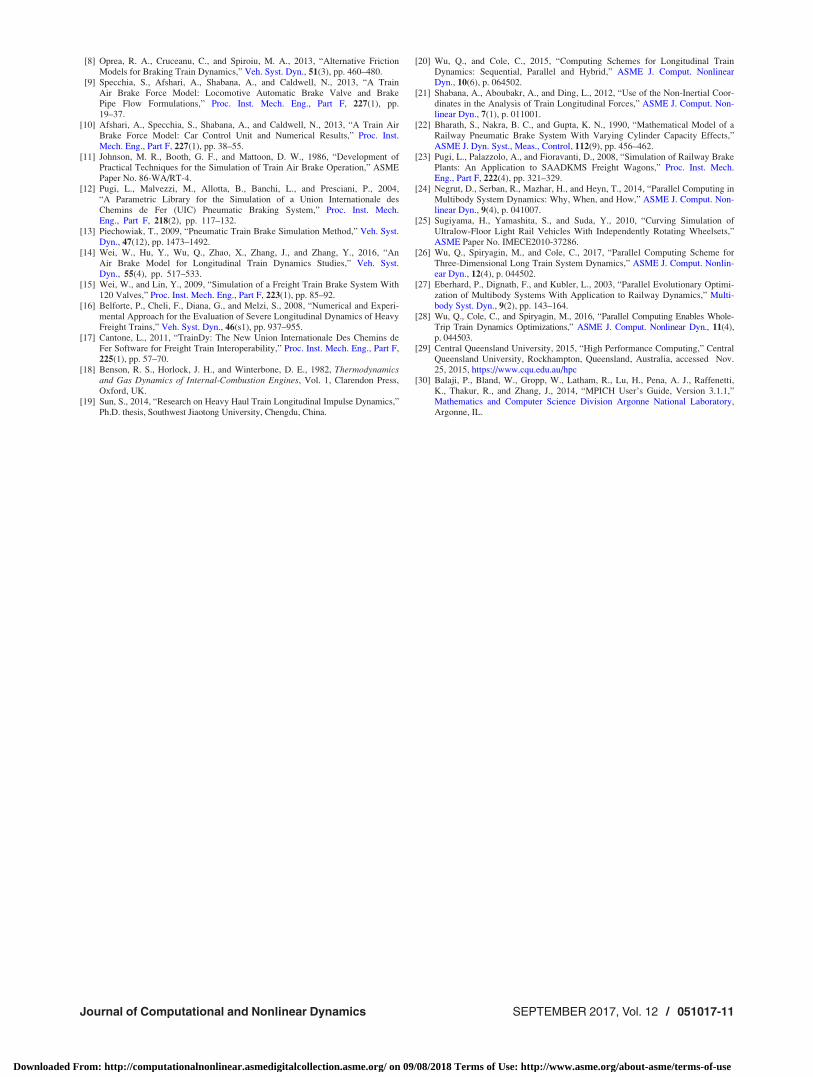
the details of air brake system behavior. This mesh size is alsorecommended by Pugi et al. [23]. In terms of numerically stiffcomponents in air brake systems, these are components that havesmall volumes, such as the upper chamber in the distributor and alow pressure brake cylinder. Figure 10 shows the simulated brakecylinder pressures in the emergency braking case using differentstep-sizes. During the simulations, the mesh sizes for brake pipesand branch pipes were 0.96 m and 0.75 m, respectively. The 20 msstep-size is about the maximum step-size for a stable solution ofthe pipe model. It can be seen that the details of push rod exten-sions are simulated only when the step-size reaches 0.1 ms. Withthe step-size of 0.1 ms, the simulation time for a 30 s brake appli-cation is 202.75 s; the simulation time is about 6.75 times slowerthan real-time.

Parallel computing is an important and effective way toimprove computational efficiency [24]. In the area of railway traindynamics, parallel computing has been successfully used toimprove computational efficiency for railway dynamics simula-tions [20,25,26] and optimizations [27,28]. In this paper, a parallelcomputing scheme as shown in Fig. 11 was developed in which

the wagon brake systems are divided into a number of groups.This figure gives an example of four wagon brake system groups(groups 0–3). The computing of each group is processed by anindependent computer core; all groups are simulated in parallel.Different cores are synchronized by time. One core (core 0) hasalso been used to compute the locomotive brake and boundaryconditions. Among the computer cores, core 0 is called the mastercore while all other cores are called slave cores. In each time-step,each slave core will project two characteristics, i.e., Riemann vari-ables (kin) into the boundaries that are at the two brake pipe endsof the wagon brake group. All entering Riemann variables (kin)are collected by the master core and then determine the corre-sponding reflecting Riemann variables (kout). Those reflectingRiemann variables are then sent to corresponding slave cores toproceed with the computing.

In this paper, all simulation codes were written in the FORTRAN

language and the Central Queensland University, high perform-ance computing system [29] was used; the message passing inter-face [30] technique was used to enable the parallel computing.The same simulations as shown in Fig. 9 were conducted using

Fig. 9 Measured and simulated results: (a) minimum brake 50 kPa reduction (measured), (b)minimum brake 50 kPa reduction (simulated), (c) full brake 170 kPa reduction (measured), (d)full brake 170 kPa reduction (simulated), (e) emergency braking (measured), and (f) emergencybraking (simulated)

051017-8 / Vol. 12, SEPTEMBER 2017 Transactions of the ASME

Downloaded From: http://computationalnonlinear.asmedigitalcollection.asme.org/ on 09/08/2018 Terms of Use: http://www.asme.org/about-asme/terms-of-use

the traditional sequential computing scheme (one core computingall brake systems) and two parallel computing schemes: (1) fourcores with four wagon groups and (2) eight cores with eightwagon groups. In the first parallel scheme, core 0 was assignedwith 30 wagons while all other cores were assigned with 40 wag-ons each. In the second parallel scheme, core 0 was assigned with

ten wagons while all other cores were assigned with 20 wagonseach. These arrangements were designed to balance the comput-ing loads among all computing cores as discussed in Ref. [20].The computing time is listed in Table 4. It can be seen that thecomputing time of the sequential scheme is about 6.7 times slowerthan real-time. Using four cores and four wagon groups candecrease the computing time by 72% and real-time simulationscan be achieved by using eight cores and eight wagon groups.

7 Conclusion

A detailed fluid dynamics air brake system was developed,which includes subsystem models for pipes, wagon brake valves,

Table 2 Comparison of brake application results

Cases

Items Wagon Sources Minimum brake Full brake Emergency brake

Average maximum cylinder pressure NA Measured 137 kPa 464 kPa 455 kPaSimulated 123 kPa 448 kPa 442 kPa

Brake application propagation rate NA Measured 224 m/s 217 m/s 254 m/sSimulated 254 m/s 245 m/s 263 m/s

Average minimum pipe pressure NA Measured 546 kPa 437 kPa 0.005 kPaSimulated 550 kPa 430 kPa 0.002 kPa

Cylinder pressure ascending time 001 Measured 85.76 s 35.35 s 8.46 sSimulated 84.61 s 34.09 s 8.97 s

075 Measured 84.24 s 99.93 s 11.92 sSimulated 86.66 s 114.74 s 11.88 s

150 Measured 81.42 s 106.20 s 16.17 sSimulated 88.89 s 115.49 s 16.70 s

Pipe pressure descending time 001 Measured 4.89 s 40.94 s 1.88 sSimulated 4.75 s 40.34 s 2.17 s

075 Measured 28.49 s 167.15 s 2.04 sSimulated 29.76 s 141.46 s 2.18 s

150 Measured 37.64 s 164.28 s 1.56 sSimulated 36.01 s 140.48 s 2.25 s

Table 3 Comparison of brake release results

Position Sources Point 1 (s) Point 2 (s) Point 3 (s)

Wagon 001 Measured 89.7 96.6 114.0Simulated 89.5 95.7 114.9

Wagon 075 Measured 95.5 102.6 119.9Simulated 96.8 103.0 121.4

Wagon 150 Measured 101.1 107.5 125.4Simulated 101.9 107.9 126.3

Fig. 10 Simulated cylinder pressures under different step-sizes

Fig. 11 Parallel computing scheme for air brake model

Journal of Computational and Nonlinear Dynamics SEPTEMBER 2017, Vol. 12 / 051017-9

Downloaded From: http://computationalnonlinear.asmedigitalcollection.asme.org/ on 09/08/2018 Terms of Use: http://www.asme.org/about-asme/terms-of-use

and locomotive brake valves. The brake pipe model is based onconservation of mass and conservation of momentum; it was solvedusing the method of characteristics. A new efficient hose connec-tion boundary condition that considers pressure loss was developed.The brake valve models have considered movements of valves andpistons as well as air flows between various volumes. A brake cyl-inder model with variable volume was also developed.

The model was validated using measured data from a test facil-ity with 150 sets of connected wagon brake systems. Simulatedresults and measured results reached an agreement with the maxi-mum difference of 15%. It is expected that these differences couldbe further reduced with further adjustment of parameters as stud-ies continue. All important features of the air brake system havebeen simulated in detail.

Parallel computing schemes were developed to improve thecomputing speed. Computing time was compared for simulationswith and without parallel computing. The computing time for theconventional sequential computing scheme was about 6.7 timesslower than real-time. Parallel computing with four computer coresdecreased the computing time by 70%. Real-time simulations wereachieved by parallel computing using eight computer cores.

Acknowledgment

The authors gratefully acknowledge the financial support fromthe State Key Laboratory of Traction Power, Open Projects(TPL1504) and the National Natural Science Foundation of China(Grant No. 51575458). The authors are also grateful to Dr. ShuleiSun (China Academy of Engineering Physics) for providingexperimental data. Acknowledgment is also made to ProfessorWei Wei (Dalian Jiaotong University) for providing advice duringthe development of the air brake model. The editing contributionof Mr. Tim McSweeney (Adjunct Research Fellow, Centre forRailway Engineering) is gratefully acknowledged.

Appendix

Two characteristics are used and they have a general expressionof

dx

dt¼ u 6 a (A1)

Along the characteristics, the following relationships exist:

dP

dt¼ @P

@tþ u 6 að Þ @P

@x(A2)

dP

dt¼ @P

@tþ u 6 að Þ @P

@x(A3)

Normalize Eqs. (4) and (5) to the following form:

a2 @q@tþ q

@u

@xþ u

@q@x¼ 0

� ��

6qa@u

@tþ u

@u

@xþ 1

q@P

@xþ f

u2

2

u

juj4

D¼ 0

!!(A4)

Then, substitute Eqs. (A1)–(A3) into Eq. (A4); the followingexpression can be derived:

dP

dt6qa

du

dt6uf

u2

2

u

juj4

D¼ 0 (A5)

Using the nondimensional conversions and Riemann variables,the following expression can be derived:

dk ¼ � k � 1

2

2fxref

D

k� bk � 1

� �2k� bð Þjk� bj 1� 2 k� bð Þ

kþ bð Þ

� �dZ (A6)

where k ¼ kI and b ¼ kII for calculating dk for kI, and k ¼ kII

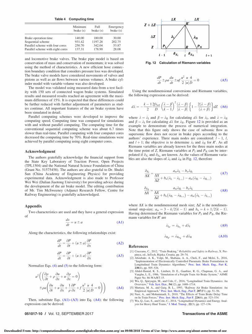
and b ¼ kI for calculating dk for kII. Figure 12 is provided as anexample to demonstrate the process of numerical integration.Note that this figure only shows the case of subsonic flow assupersonic flow does not occur in brake pipes according to theauthors’ experience. Three main nodes are considered: l� 1, l,and lþ 1; the objective is to determine kI and kII for R0. As allRiemann variables are already known for the three main nodes atthe time point of Z, Riemann variables at PI and PII can be inter-polated if dXI

and dXIIare known. As the values of Riemann varia-

bles are also the slopes of kI and kII in Fig. 12, therefore

dXI

DX¼ amkIl

� bnkIIl

DX

DZþ bn kIl

� kIl�1ð Þ � am kIIl� kIIl�1ð Þ

(A7)

dXII

DX¼ amkIIl

� bnkIl

DX

DZþ bn kIIl

� kIIlþ1

� �� am kIl

� kIlþ1

� � (A8)

where DX is the nondimensional mesh size; DZ is the nondimen-sional step-size; am ¼ 3� k=2 k � 1ð Þ and bn ¼ k þ 1=2 k � 1ð Þ.Having determined the Riemann variables for PI and PII, the Rie-mann variables for R0 are

kIR0 ¼ kIPIþ dkI (A9)

kIIR0 ¼ kIIPIIþ dkII (A10)

References[1] Cruceanu, C., 2012, “Train Braking,” Reliability and Safety in Railway, X. Per-

pinya, ed., InTech, Rijeka, Croatia, pp. 29–74.[2] Aboubakr, A. K., Volpi, M., Shabana, A. A., Cheli, F., and Melzi, S., 2016,

“Implementation of Electronically Controlled Pneumatic Brake Formulation inLongitudinal Train Dynamics Algorithms,” Proc. Inst. Mech. Eng., Part K,230(4), pp. 505–526.

[3] Abdol-Hamid, K. S., Limbert, D. E., Gauthier, R. G., Chapman, G. A., andVaughn, L. E., 1986, “Simulation of a Freight Train Air Brake System,” ASMEPaper No. 86-WA/RT-15.

[4] Wu, Q., Spiryagin, M., and Cole, C., 2016, “Longitudinal Train Dynamics: AnOverview,” Veh. Syst. Dyn., 54(12), pp. 1688–1714.

[5] Murtaza, M. A., and Garg, B. L., 1993, “Railway Air Brake Simulation: AnEmpirical Approach,” Proc. Inst. Mech. Eng., Part F, 207(F1), pp. 51–56.

[6] Nasr, A., and Mohammadi, S., 2010, “The Effects of Train Brake Delay Timeon In-Train Forces,” Proc. Inst. Mech. Eng., Part F, 224(6), pp. 523–534.

[7] Wu, Q., Luo, S., and Cole, C., 2014, “Longitudinal Dynamics and Energy Anal-ysis for Heavy Haul Trains,” J. Mod. Transp., 22(3), pp. 127–136.

Fig. 12 Calculation of Riemann variables

Table 4 Computing time

Minimumbrake (s)

Fullbrake (s)

Emergencybrake (s)

Brake operation time 140.00 180.00 30.00Sequential scheme 931.42 1197.28 202.75Parallel scheme with four cores 250.70 342.04 53.87Parallel scheme with eight cores 137.31 178.90 28.08

051017-10 / Vol. 12, SEPTEMBER 2017 Transactions of the ASME

Downloaded From: http://computationalnonlinear.asmedigitalcollection.asme.org/ on 09/08/2018 Terms of Use: http://www.asme.org/about-asme/terms-of-use

[8] Oprea, R. A., Cruceanu, C., and Spiroiu, M. A., 2013, “Alternative FrictionModels for Braking Train Dynamics,” Veh. Syst. Dyn., 51(3), pp. 460–480.

[9] Specchia, S., Afshari, A., Shabana, A., and Caldwell, N., 2013, “A TrainAir Brake Force Model: Locomotive Automatic Brake Valve and BrakePipe Flow Formulations,” Proc. Inst. Mech. Eng., Part F, 227(1), pp.19–37.

[10] Afshari, A., Specchia, S., Shabana, A., and Caldwell, N., 2013, “A Train AirBrake Force Model: Car Control Unit and Numerical Results,” Proc. Inst.Mech. Eng., Part F, 227(1), pp. 38–55.

[11] Johnson, M. R., Booth, G. F., and Mattoon, D. W., 1986, “Development ofPractical Techniques for the Simulation of Train Air Brake Operation,” ASMEPaper No. 86-WA/RT-4.

[12] Pugi, L., Malvezzi, M., Allotta, B., Banchi, L., and Presciani, P., 2004,“A Parametric Library for the Simulation of a Union Internationale desChemins de Fer (UIC) Pneumatic Braking System,” Proc. Inst. Mech.Eng., Part F, 218(2), pp. 117–132.

[13] Piechowiak, T., 2009, “Pneumatic Train Brake Simulation Method,” Veh. Syst.Dyn., 47(12), pp. 1473–1492.

[14] Wei, W., Hu, Y., Wu, Q., Zhao, X., Zhang, J., and Zhang, Y., 2016, “AnAir Brake Model for Longitudinal Train Dynamics Studies,” Veh. Syst.Dyn., 55(4), pp. 517–533.

[15] Wei, W., and Lin, Y., 2009, “Simulation of a Freight Train Brake System With120 Valves,” Proc. Inst. Mech. Eng., Part F, 223(1), pp. 85–92.

[16] Belforte, P., Cheli, F., Diana, G., and Melzi, S., 2008, “Numerical and Experi-mental Approach for the Evaluation of Severe Longitudinal Dynamics of HeavyFreight Trains,” Veh. Syst. Dyn., 46(s1), pp. 937–955.

[17] Cantone, L., 2011, “TrainDy: The New Union Internationale Des Chemins deFer Software for Freight Train Interoperability,” Proc. Inst. Mech. Eng., Part F,225(1), pp. 57–70.

[18] Benson, R. S., Horlock, J. H., and Winterbone, D. E., 1982, Thermodynamicsand Gas Dynamics of Internal-Combustion Engines, Vol. 1, Clarendon Press,Oxford, UK.

[19] Sun, S., 2014, “Research on Heavy Haul Train Longitudinal Impulse Dynamics,”Ph.D. thesis, Southwest Jiaotong University, Chengdu, China.

[20] Wu, Q., and Cole, C., 2015, “Computing Schemes for Longitudinal TrainDynamics: Sequential, Parallel and Hybrid,” ASME J. Comput. NonlinearDyn., 10(6), p. 064502.

[21] Shabana, A., Aboubakr, A., and Ding, L., 2012, “Use of the Non-Inertial Coor-dinates in the Analysis of Train Longitudinal Forces,” ASME J. Comput. Non-linear Dyn., 7(1), p. 011001.

[22] Bharath, S., Nakra, B. C., and Gupta, K. N., 1990, “Mathematical Model of aRailway Pneumatic Brake System With Varying Cylinder Capacity Effects,”ASME J. Dyn. Syst., Meas., Control, 112(9), pp. 456–462.

[23] Pugi, L., Palazzolo, A., and Fioravanti, D., 2008, “Simulation of Railway BrakePlants: An Application to SAADKMS Freight Wagons,” Proc. Inst. Mech.Eng., Part F, 222(4), pp. 321–329.

[24] Negrut, D., Serban, R., Mazhar, H., and Heyn, T., 2014, “Parallel Computing inMultibody System Dynamics: Why, When, and How,” ASME J. Comput. Non-linear Dyn., 9(4), p. 041007.

[25] Sugiyama, H., Yamashita, S., and Suda, Y., 2010, “Curving Simulation ofUltralow-Floor Light Rail Vehicles With Independently Rotating Wheelsets,”ASME Paper No. IMECE2010-37286.

[26] Wu, Q., Spiryagin, M., and Cole, C., 2017, “Parallel Computing Scheme forThree-Dimensional Long Train System Dynamics,” ASME J. Comput. Nonlin-ear Dyn., 12(4), p. 044502.

[27] Eberhard, P., Dignath, F., and Kubler, L., 2003, “Parallel Evolutionary Optimi-zation of Multibody Systems With Application to Railway Dynamics,” Multi-body Syst. Dyn., 9(2), pp. 143–164.

[28] Wu, Q., Cole, C., and Spiryagin, M., 2016, “Parallel Computing Enables Whole-Trip Train Dynamics Optimizations,” ASME J. Comput. Nonlinear Dyn., 11(4),p. 044503.

[29] Central Queensland University, 2015, “High Performance Computing,” CentralQueensland University, Rockhampton, Queensland, Australia, accessed Nov.25, 2015, https://www.cqu.edu.au/hpc

[30] Balaji, P., Bland, W., Gropp, W., Latham, R., Lu, H., Pena, A. J., Raffenetti,K., Thakur, R., and Zhang, J., 2014, “MPICH User’s Guide, Version 3.1.1,”Mathematics and Computer Science Division Argonne National Laboratory,Argonne, IL.

Journal of Computational and Nonlinear Dynamics SEPTEMBER 2017, Vol. 12 / 051017-11

Downloaded From: http://computationalnonlinear.asmedigitalcollection.asme.org/ on 09/08/2018 Terms of Use: http://www.asme.org/about-asme/terms-of-use