CENTER FOR BIOLOGICAL SEQUENCE ANALYSIS Brief Introduction to the Theory of Evolution Anders Gorm...

CE

NT

ER

FO

R B

IOLO

GIC

AL

SE

QU

EN

CE

AN

ALY

SIS Brief Introduction to

the Theory of Evolution

Anders Gorm PedersenAnders Gorm Pedersen

Molecular Evolution GroupMolecular Evolution Group

Center for Biological Sequence Center for Biological Sequence AnalysisAnalysis

[email protected]@cbs.dtu.dk

CE

NT

ER

FO

R B

IOLO

GIC

AL

SE

QU

EN

CE

AN

ALY

SIS

Classification: Linnaeus

Carl LinnaeusCarl Linnaeus1707-17781707-1778

CE

NT

ER

FO

R B

IOLO

GIC

AL

SE

QU

EN

CE

AN

ALY

SIS

Classification: Linnaeus

• Hierarchical systemHierarchical system

– KingdomKingdom– PhylumPhylum– ClassClass– OrderOrder– FamilyFamily– GenusGenus– SpeciesSpecies

CE

NT

ER

FO

R B

IOLO

GIC

AL

SE

QU

EN

CE

AN

ALY

SIS

Classification depicted as a tree

CE

NT

ER

FO

R B

IOLO

GIC

AL

SE

QU

EN

CE

AN

ALY

SIS

Classification depicted as a tree

SpeciesSpecies GenusGenus FamilyFamily OrderOrder ClassClass

CE

NT

ER

FO

R B

IOLO

GIC

AL

SE

QU

EN

CE

AN

ALY

SIS

Theory of evolution

Charles DarwinCharles Darwin1809-18821809-1882

CE

NT

ER

FO

R B

IOLO

GIC

AL

SE

QU

EN

CE

AN

ALY

SIS

Phylogenetic basis of systematics

• LinnaeusLinnaeus: : Ordering principle is God.Ordering principle is God.

• DarwinDarwin: : Ordering principle is shared Ordering principle is shared descent from common descent from common ancestors.ancestors.

• Today, systematics is Today, systematics is explicitly based on explicitly based on phylogeny.phylogeny.

CE

NT

ER

FO

R B

IOLO

GIC

AL

SE

QU

EN

CE

AN

ALY

SIS

Darwin’s four postulates

• More young are produced each generation than can More young are produced each generation than can survive to reproduce.survive to reproduce.

• Individuals in a population vary in their Individuals in a population vary in their characteristics.characteristics.

• Some differences among individuals are based on Some differences among individuals are based on genetic differences.genetic differences.

• Individuals with favorable characteristics have Individuals with favorable characteristics have higher rates of survival and reproduction.higher rates of survival and reproduction.

• Evolution by means of natural selectionEvolution by means of natural selection• Presence of ”design-like” features in organisms:Presence of ”design-like” features in organisms:• quite often features are there “for a quite often features are there “for a

reason”reason”

CE

NT

ER

FO

R B

IOLO

GIC

AL

SE

QU

EN

CE

AN

ALY

SIS

Theory of evolution as the basis of biological

understanding

”Nothing in biology makes sense, except in the light of evolution.

Without that light it becomes a pile of sundry facts - some of them interesting or curious but making no meaningful picture as a whole”

T. Dobzhansky

CE

NT

ER

FO

R B

IOLO

GIC

AL

SE

QU

EN

CE

AN

ALY

SIS Phylogenetic Reconstruction:

Distance Matrix Methods

Anders Gorm PedersenAnders Gorm Pedersen

Molecular Evolution GroupMolecular Evolution Group

Center for Biological Sequence AnalysisCenter for Biological Sequence Analysis

Technical University of DenmarkTechnical University of Denmark

[email protected]@cbs.dtu.dk

CE

NT

ER

FO

R B

IOLO

GIC

AL

SE

QU

EN

CE

AN

ALY

SIS

Trees: terminology

CE

NT

ER

FO

R B

IOLO

GIC

AL

SE

QU

EN

CE

AN

ALY

SIS

Trees: representations

Three different representations of the same tree

CE

NT

ER

FO

R B

IOLO

GIC

AL

SE

QU

EN

CE

AN

ALY

SIS

Trees: rooted vs. unrooted

• A rooted tree has a single node (the root) that represents a point in time that is earlier than any other node in the tree.

• A rooted tree has directionality (nodes can be ordered in terms of “earlier” or “later”).

• In the rooted tree, distance between two nodes is represented along the time-axis only (the second axis just helps spread out the leafs)

Early Late

CE

NT

ER

FO

R B

IOLO

GIC

AL

SE

QU

EN

CE

AN

ALY

SIS

Trees: rooted vs. unrooted

• In unrooted trees there is no directionality: we do not In unrooted trees there is no directionality: we do not know if a node is earlier or later than another nodeknow if a node is earlier or later than another node

• Distance along branches directly represents node distanceDistance along branches directly represents node distance

CE

NT

ER

FO

R B

IOLO

GIC

AL

SE

QU

EN

CE

AN

ALY

SIS

Reconstructing a tree using non-contemporaneous data

CE

NT

ER

FO

R B

IOLO

GIC

AL

SE

QU

EN

CE

AN

ALY

SIS

Reconstructing a tree using present-day data

CE

NT

ER

FO

R B

IOLO

GIC

AL

SE

QU

EN

CE

AN

ALY

SIS

Molecular phylogeny

AA A G C G T T G G G C A A A G C G T T G G G C A A

BB A G C G T T T G G C A A A G C G T T T G G C A A

CC A G C T T T G T G C A A A G C T T T G T G C A A

DD A G C T T T T T G C A A A G C T T T T T G C A A

1 2 3 1 2 3

• DNA and protein DNA and protein sequences sequences

• Homologous characters Homologous characters inferred from alignment.inferred from alignment.

• Other molecular data: Other molecular data: absence/presence of absence/presence of restriction sites, DNA restriction sites, DNA hybridization data, hybridization data, antibody cross-antibody cross-reactivity, etc. (but reactivity, etc. (but losing importance due to losing importance due to cheap, efficient cheap, efficient sequencing).sequencing).

CE

NT

ER

FO

R B

IOLO

GIC

AL

SE

QU

EN

CE

AN

ALY

SIS

Morphology vs. molecular data

African white-backed vulture(old world vulture)

Andean condor (new world vulture)

New and old world vultures seem to be closely related based on morphology.

Molecular data indicates that old world vultures are related to birds of prey (falcons, hawks, etc.) while new world vultures are more closely related to storks

Similar features presumably the result of convergent evolution

CE

NT

ER

FO

R B

IOLO

GIC

AL

SE

QU

EN

CE

AN

ALY

SIS

Molecular data: single-celled organisms

Molecular data useful for analyzing single-celled organisms (which have only few prominent morphological features).

CE

NT

ER

FO

R B

IOLO

GIC

AL

SE

QU

EN

CE

AN

ALY

SIS

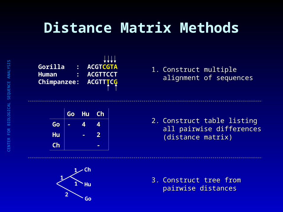
Distance Matrix Methods

1.1. Construct multiple Construct multiple alignment of sequencesalignment of sequences

2.2. Construct table listing Construct table listing all pairwise all pairwise differences (distance differences (distance matrix)matrix)

3.3. Construct tree from Construct tree from pairwise distancespairwise distances

Gorilla : ACGTCGTAHuman : ACGTTCCTChimpanzee: ACGTTTCG

GoGo HuHu ChCh

GoGo -- 44 44

HuHu -- 22

ChCh --

Go

Hu

Ch

2

11

1

CE

NT

ER

FO

R B

IOLO

GIC

AL

SE

QU

EN

CE

AN

ALY

SIS

Finding Optimal Branch Lengths

SS11 SS22 SS33 SS44

SS11 -- DD1212 DD1313 DD1414

SS22 -- DD2323 DD2424

SS33 -- DD3434

SS44 --Observed distance

S1

S3

S2

S4

a

b

c

d e

Distance along tree

D12 d12 = a + b + cD13 d13 = a + dD14 d14 = a + b + eD23 d23 = d + b + cD24 d24 = c + eD34 d34 = d + b + e

Goal:

CE

NT

ER

FO

R B

IOLO

GIC

AL

SE

QU

EN

CE

AN

ALY

SIS

Exercise (handout)

• Construct distance matrix (count different Construct distance matrix (count different positions)positions)

• Reconstruct tree and find best set of Reconstruct tree and find best set of branch lengthsbranch lengths

CE

NT

ER

FO

R B

IOLO

GIC

AL

SE

QU

EN

CE

AN

ALY

SIS

Optimal Branch Lengths: Least Squares

• Fit between given tree Fit between given tree and observed distances and observed distances can be expressed as can be expressed as “sum of squared “sum of squared differences”:differences”:

Q = Q = (D(Dijij - d - dijij))22

• Find branch lengths Find branch lengths that minimize Q - this that minimize Q - this is the optimal set of is the optimal set of branch lengths for this branch lengths for this tree.tree.

S1

S3

S2

S4

a

b

c

d e

Distance along tree


Goal:

j>i

CE

NT

ER

FO

R B

IOLO

GIC

AL

SE

QU

EN

CE

AN

ALY

SIS

Optimal Branch Lengths: Least Squares

• Longer distances Longer distances associated with larger associated with larger errorserrors

• Squared deviation may be Squared deviation may be weighted so longer weighted so longer branches contribute less branches contribute less to Q:to Q:

Q = Q = (D(Dijij - d - dijij))22

• Power (n) is typically 1 or 2

S1

S3

S2

S4

a

b

c

d e

Distance along tree


Goal:Dij

n

CE

NT

ER

FO

R B

IOLO

GIC

AL

SE

QU

EN

CE

AN

ALY

SIS

Least Squares Optimality Criterion

• Search through all (or many) tree topologiesSearch through all (or many) tree topologies

• For each investigated tree, find best branch For each investigated tree, find best branch lengths using least squares criterionlengths using least squares criterion

• Among all investigated trees, the best tree Among all investigated trees, the best tree is the one with the smallest sum of squared is the one with the smallest sum of squared errors. errors.

• Least squares criterion used both for Least squares criterion used both for finding branch lengths on individual trees, finding branch lengths on individual trees, and for finding best tree.and for finding best tree.

CE

NT

ER

FO

R B

IOLO

GIC

AL

SE

QU

EN

CE

AN

ALY

SIS

Minimum Evolution Optimality Criterion

• Search through all (or many) tree topologiesSearch through all (or many) tree topologies

• For each investigated tree, find best branch For each investigated tree, find best branch lengths using least squares criterionlengths using least squares criterion

• Among all investigated trees, the best tree Among all investigated trees, the best tree is the one with the smallest sum of branch is the one with the smallest sum of branch lengths (the shortest tree).lengths (the shortest tree).

• Least squares criterion used for finding Least squares criterion used for finding branch lengths on individual trees, minimum branch lengths on individual trees, minimum tree length used for finding best tree.tree length used for finding best tree.

CE

NT

ER

FO

R B

IOLO

GIC

AL

SE

QU

EN

CE

AN

ALY

SIS

How many unrooted trees are there?

• There is only one way There is only one way of con-structing the of con-structing the first tree. This tree first tree. This tree has 3 tips and 3 has 3 tips and 3 branchesbranches

• Each time an extra taxon Each time an extra taxon is added, two branches is added, two branches are created.are created.

• A tree with n tips will A tree with n tips will therefore have the therefore have the following number of following number of branches:branches:

nnbranchesbranches = 3+(n-3)*2= 3+(n-3)*2= 3+2n-6= 3+2n-6= 2n-3= 2n-3

A B

C

A B

C

D

CE

NT

ER

FO

R B

IOLO

GIC

AL

SE

QU

EN

CE

AN

ALY

SIS

How many unrooted trees are there?

• A tree with n tips has A tree with n tips has 2n-3 branches2n-3 branches

• For each tree with n For each tree with n tips, we can therefore tips, we can therefore construct 2n-3 derived construct 2n-3 derived trees (with n+1 tips). trees (with n+1 tips).

• The number of unrooted The number of unrooted trees with n+1 tips is trees with n+1 tips is therefore:therefore:

(2i-3) = 1 x 3 x 5 x (2i-3) = 1 x 3 x 5 x 7 x ...7 x ...i=2

n

CE

NT

ER

FO

R B

IOLO

GIC

AL

SE

QU

EN

CE

AN

ALY

SIS

Exhaustive search impossible for large data sets

No. No. taxataxa

No. treesNo. trees

33 11

44 33

55 1515

66 105105

77 945945

88 10,39510,395

99 135,135135,135

1010 2,027,0252,027,025

1111 34,459,42534,459,425

1212 654,729,075654,729,075

1313 13,749,310,57513,749,310,575

1414 316,234,143,225316,234,143,225

1515 7,905,853,580,6257,905,853,580,625

CE

NT

ER

FO

R B

IOLO

GIC

AL

SE

QU

EN

CE

AN

ALY

SIS

Heuristic search

1.1. Construct initial tree; determine sum of squaresConstruct initial tree; determine sum of squares

2.2. Construct set of “neighboring trees” by making small Construct set of “neighboring trees” by making small rearrangements of initial tree; determine sum of rearrangements of initial tree; determine sum of squares for each neighborsquares for each neighbor

3.3. If any of the neighboring trees are better than the If any of the neighboring trees are better than the initial tree, then select it/them and use as starting initial tree, then select it/them and use as starting point for new round of rearrangements. (Possibly point for new round of rearrangements. (Possibly several neighbors are equally good)several neighbors are equally good)

4.4. Repeat steps 2+3 until you have found a tree that is Repeat steps 2+3 until you have found a tree that is better than all of its neighbors.better than all of its neighbors.

5.5. This tree is a “local optimum” (not necessarily a This tree is a “local optimum” (not necessarily a global optimum!) global optimum!)

CE

NT

ER

FO

R B

IOLO

GIC

AL

SE

QU

EN

CE

AN

ALY

SIS

Heuristic search: hill-climbing

CE

NT

ER

FO

R B

IOLO

GIC

AL

SE

QU

EN

CE

AN

ALY

SIS

Heuristic search: local vs. global optimum

QuickTime™ and aTIFF (Uncompressed) decompressor

are needed to see this picture.

CE

NT

ER

FO

R B

IOLO

GIC

AL

SE

QU

EN

CE

AN

ALY

SIS

Types of rearrangement I: nearest neighbor interchange

(NNI)Original tree

Two neighbors per internal branch: tree with n tips has 2(n-3) neighbors(For example, a tree with 20 tips has 34 neighbbors)

CE

NT

ER

FO

R B

IOLO

GIC

AL

SE

QU

EN

CE

AN

ALY

SIS

Types of rearrangement II: subtree pruning and regrafting

(SPR)

CE

NT

ER

FO

R B

IOLO

GIC

AL

SE

QU

EN

CE

AN

ALY

SIS

Types of rearrangement III: tree bisection and reconnection (TBR)

CE

NT

ER

FO

R B

IOLO

GIC

AL

SE

QU

EN

CE

AN

ALY

SIS

Clustering Algorithms

• Starting point: Distance matrixStarting point: Distance matrix

• Cluster least different pair of sequences:Cluster least different pair of sequences:– Tree: pair connected to common ancestral node, compute Tree: pair connected to common ancestral node, compute

branch lengths from ancestral node to both descendantsbranch lengths from ancestral node to both descendants

– Distance matrix: combine two entries into one. Compute Distance matrix: combine two entries into one. Compute

new distance matrix, by finding distance from new node new distance matrix, by finding distance from new node to all other nodesto all other nodes

• Repeat until all nodes are linkedRepeat until all nodes are linked

• Results in only one tree, there is no measure Results in only one tree, there is no measure of tree-goodness.of tree-goodness.

CE

NT

ER

FO

R B

IOLO

GIC

AL

SE

QU

EN

CE

AN

ALY

SIS

Neighbor Joining Algorithm

• For each tip compute For each tip compute uuii = = jj DDijij/(n-2)/(n-2)

(this is essentially the average distance to all other (this is essentially the average distance to all other tips, except the denominator is n-2 instead of n)tips, except the denominator is n-2 instead of n)

• Find the pair of tips, i and j, where Find the pair of tips, i and j, where DDijij-u-uii-u-ujj is smallest is smallest

• Connect the tips i and j, forming a new ancestral node. The Connect the tips i and j, forming a new ancestral node. The branch lengths from the ancestral node to i and j are:branch lengths from the ancestral node to i and j are:

vvii = 0.5 D = 0.5 Dijij + 0.5 (u + 0.5 (uii-u-ujj))

vvjj = 0.5 D = 0.5 Dijij + 0.5 (u + 0.5 (ujj-u-uii))

• Update the distance matrix: Compute distance between new Update the distance matrix: Compute distance between new node and each remaining tip as follows:node and each remaining tip as follows:

DDij,kij,k = (D = (Dikik+D+Djkjk-D-Dijij)/2)/2

• Replace tips i and j by the new node which is now treated Replace tips i and j by the new node which is now treated as a tipas a tip

• Repeat until only two nodes remain.Repeat until only two nodes remain.

CE

NT

ER

FO

R B

IOLO

GIC

AL

SE

QU

EN

CE

AN

ALY

SIS

Superimposed Substitutions

• Actual number of Actual number of

evolutionary events:evolutionary events:55

• Observed number of Observed number of

differences:differences: 22

• Distance is (almost) Distance is (almost) always underestimatedalways underestimated

ACGGTGC

C T

GCGGTGA

CE

NT

ER

FO

R B

IOLO

GIC

AL

SE

QU

EN

CE

AN

ALY

SIS

Model-based correction for superimposed substitutions

• Goal: try to infer the real number of Goal: try to infer the real number of evolutionary events (the real distance) evolutionary events (the real distance) based onbased on

1.1. Observed data (sequence alignment)Observed data (sequence alignment)

2.2. A model of how evolution occursA model of how evolution occurs

CE

NT

ER

FO

R B

IOLO

GIC

AL

SE

QU

EN

CE

AN

ALY

SIS

Jukes and Cantor Model

• Four nucleotides assumed Four nucleotides assumed to be equally frequent to be equally frequent (f=0.25)(f=0.25)

• All 12 substitution rates All 12 substitution rates assumed to be equalassumed to be equal

• Under this model the Under this model the corrected distance is:corrected distance is:

DDJCJC = -0.75 x ln(1-1.33 x = -0.75 x ln(1-1.33 x DDOBSOBS))

• For instance:For instance:

DDOBSOBS=0.43 => D=0.43 => DJCJC=0.64=0.64

A C G T

A -3

C -3

G -3

T -3

CE

NT

ER

FO

R B

IOLO

GIC

AL

SE

QU

EN

CE

AN

ALY

SIS

Other models of evolution

CE

NT

ER

FO

R B

IOLO

GIC

AL

SE

QU

EN

CE

AN

ALY

SIS


• For each tip compute For each tip compute uuii = = jj DDijij/(n-2)/(n-2)

(this is essentially the average distance to all other (this is essentially the average distance to all other tips, except the denominator is n-2 instead of n)tips, except the denominator is n-2 instead of n)

• Find the pair of tips, i and j, where Find the pair of tips, i and j, where DDijij-u-uii-u-ujj is smallest is smallest

• Connect the tips i and j, forming a new ancestral node. The Connect the tips i and j, forming a new ancestral node. The branch lengths from the ancestral node to i and j are:branch lengths from the ancestral node to i and j are:

vvii = 0.5 D = 0.5 Dijij + 0.5 (u + 0.5 (uii-u-ujj))

vvjj = 0.5 D = 0.5 Dijij + 0.5 (u + 0.5 (ujj-u-uii))

• Update the distance matrix: Compute distance between new Update the distance matrix: Compute distance between new node and each remaining tip as follows:node and each remaining tip as follows:

DDij,kij,k = (D = (Dikik+D+Djkjk-D-Dijij)/2)/2

• Replace tips i and j by the new node which is now treated Replace tips i and j by the new node which is now treated as a tipas a tip

• Repeat until only two nodes remain.Repeat until only two nodes remain.

CE

NT

ER

FO

R B

IOLO

GIC

AL

SE

QU

EN

CE

AN

ALY

SIS


AA BB CC DD

AA -- 1717 2121 2727

BB -- 1212 1818

CC -- 1414

DD --

CE

NT

ER

FO

R B

IOLO

GIC

AL

SE

QU

EN

CE

AN

ALY

SIS


AA BB CC DD

AA -- 1717 2121 2727

BB -- 1212 1818

CC -- 1414

DD --

ii uuii

AA (17+21+27)/2=32.5(17+21+27)/2=32.5

BB (17+12+18)/2=23.5(17+12+18)/2=23.5

CC (21+12+14)/2=23.5(21+12+14)/2=23.5

DD (27+18+14)/2=29.5(27+18+14)/2=29.5

CE

NT

ER

FO

R B

IOLO

GIC

AL

SE

QU

EN

CE

AN

ALY

SIS


AA BB CC DD

AA -- 1717 2121 2727

BB -- 1212 1818

CC -- 1414

DD --

ii uuii

AA (17+21+27)/2=32.5(17+21+27)/2=32.5

BB (17+12+18)/2=23.5(17+12+18)/2=23.5

CC (21+12+14)/2=23.5(21+12+14)/2=23.5

DD (27+18+14)/2=29.5(27+18+14)/2=29.5

AA BB CC DD

AA -- -39-39 -35-35 -35-35

BB -- -35-35 -35-35

CC -- -39-39

DD --

Dij-ui-uj

CE

NT

ER

FO

R B

IOLO

GIC

AL

SE

QU

EN

CE

AN

ALY

SIS


AA BB CC DD

AA -- 1717 2121 2727

BB -- 1212 1818

CC -- 1414

DD --

ii uuii

AA (17+21+27)/2=32.5(17+21+27)/2=32.5

BB (17+12+18)/2=23.5(17+12+18)/2=23.5

CC (21+12+14)/2=23.5(21+12+14)/2=23.5

DD (27+18+14)/2=29.5(27+18+14)/2=29.5

AA BB CC DD

AA -- -39-39 -35-35 -35-35

BB -- -35-35 -35-35

CC -- -39-39

DD --

Dij-ui-uj

C D

X

CE

NT

ER

FO

R B

IOLO

GIC

AL

SE

QU

EN

CE

AN

ALY

SIS


AA BB CC DD

AA -- 1717 2121 2727

BB -- 1212 1818

CC -- 1414

DD --

ii uuii

AA (17+21+27)/2=32.5(17+21+27)/2=32.5

BB (17+12+18)/2=23.5(17+12+18)/2=23.5

CC (21+12+14)/2=23.5(21+12+14)/2=23.5

DD (27+18+14)/2=29.5(27+18+14)/2=29.5

AA BB CC DD

AA -- -39-39 -35-35 -35-35

BB -- -35-35 -35-35

CC -- -39-39

DD --

Dij-ui-uj

C D

vC = 0.5 x 14 + 0.5 x (23.5-29.5) = 4vD = 0.5 x 14 + 0.5 x (29.5-23.5) = 10

4 10X

CE

NT

ER

FO

R B

IOLO

GIC

AL

SE

QU

EN

CE

AN

ALY

SIS


AA BB CC DD XX

AA -- 1717 2121 2727

BB -- 1212 1818

CC -- 1414

DD --

XX --

C D

4 10X

CE

NT

ER

FO

R B

IOLO

GIC

AL

SE

QU

EN

CE

AN

ALY

SIS


AA BB CC DD XX

AA -- 1717 2121 2727

BB -- 1212 1818

CC -- 1414

DD --

XX --

C D

4 10X

DXA = (DCA + DDA - DCD)/2 = (21 + 27 - 14)/2 = 17

DXB = (DCB + DDB - DCD)/2 = (12 + 18 - 14)/2 = 8

CE

NT

ER

FO

R B

IOLO

GIC

AL

SE

QU

EN

CE

AN

ALY

SIS


AA BB CC DD XX

AA -- 1717 2121 2727 1717

BB -- 1212 1818 88

CC -- 1414

DD --

XX --

C D

4 10X

DXA = (DCA + DDA - DCD)/2 = (21 + 27 - 14)/2 = 17

DXB = (DCB + DDB - DCD)/2 = (12 + 18 - 14)/2 = 8

CE

NT

ER

FO

R B

IOLO

GIC

AL

SE

QU

EN

CE

AN

ALY

SIS


AA BB XX

AA -- 1717 1717

BB -- 88

XX --

C D

4 10X

DXA = (DCA + DDA - DCD)/2 = (21 + 27 - 14)/2 = 17

DXB = (DCB + DDB - DCD)/2 = (12 + 18 - 14)/2 = 8

CE

NT

ER

FO

R B

IOLO

GIC

AL

SE

QU

EN

CE

AN

ALY

SIS


AA BB XX

AA -- 1717 1717

BB -- 88

XX --

C D

4 10X

ii uuii

AA (17+17)/1 = 34(17+17)/1 = 34

BB (17+8)/1 = 25(17+8)/1 = 25

XX (17+8)/1 = 25(17+8)/1 = 25

CE

NT

ER

FO

R B

IOLO

GIC

AL

SE

QU

EN

CE

AN

ALY

SIS


AA BB XX

AA -- 1717 1717

BB -- 88

XX --

C D

4 10X

AA BB XX

AA -- -42-42 -28-28

BB -- -28-28

XX --

Dij-ui-uj

ii uuii

AA (17+17)/1 = 34(17+17)/1 = 34

BB (17+8)/1 = 25(17+8)/1 = 25

XX (17+8)/1 = 25(17+8)/1 = 25

CE

NT

ER

FO

R B

IOLO

GIC

AL

SE

QU

EN

CE

AN

ALY

SIS


AA BB XX

AA -- 1717 1717

BB -- 88

XX --

C D

4 10X

Dij-ui-uj

AA BB XX

AA -- --4242 -28-28

BB -- -28-28

XX --

ii uuii

AA (17+17)/1 = 34(17+17)/1 = 34

BB (17+8)/1 = 25(17+8)/1 = 25

XX (17+8)/1 = 25(17+8)/1 = 25

CE

NT

ER

FO

R B

IOLO

GIC

AL

SE

QU

EN

CE

AN

ALY

SIS


AA BB XX

AA -- 1717 1717

BB -- 88

XX --

C D

4 10X

Dij-ui-uj

AA BB XX

AA -- --4242 -28-28

BB -- -28-28

XX --

ii uuii

AA (17+17)/1 = 34(17+17)/1 = 34

BB (17+8)/1 = 25(17+8)/1 = 25

XX (17+8)/1 = 25(17+8)/1 = 25

vA = 0.5 x 17 + 0.5 x (34-25) = 13vD = 0.5 x 17 + 0.5 x (25-34) = 4

A B

Y413

CE

NT

ER

FO

R B

IOLO

GIC

AL

SE

QU

EN

CE

AN

ALY

SIS


AA BB XX YY

AA -- 1717 1717

BB -- 88

XX --

YY

C D

4 10X

A B

Y413

CE

NT

ER

FO

R B

IOLO

GIC

AL

SE

QU

EN

CE

AN

ALY

SIS


AA BB XX YY

AA -- 1717 1717

BB -- 88

XX -- 44

YY

C D

4 10X

A B

Y413

DYX = (DAX + DBX - DAB)/2 = (17 + 8 - 17)/2 = 4

CE

NT

ER

FO

R B

IOLO

GIC

AL

SE

QU

EN

CE

AN

ALY

SIS


XX YY

XX -- 44

YY --

C D

4 10X

A B

Y413

DYX = (DAX + DBX - DAB)/2 = (17 + 8 - 17)/2 = 4

CE

NT

ER

FO

R B

IOLO

GIC

AL

SE

QU

EN

CE

AN

ALY

SIS


XX YY

XX -- 44

YY --

C D

4 10

A B

413

4

DYX = (DAX + DBX - DAB)/2 = (17 + 8 - 17)/2 = 4

CE

NT

ER

FO

R B

IOLO

GIC

AL

SE

QU

EN

CE

AN

ALY

SIS


C

D

A

BAA BB CC DD

AA -- 1717 2121 2727

BB -- 1212 1818

CC -- 1414

DD -- 10

4

13

4

4

CENTER FOR BIOLOGICAL SEQUENCE ANALYSIS Brief Introduction to the Theory of Evolution Anders Gorm...

Documents

Transcript of CENTER FOR BIOLOGICAL SEQUENCE ANALYSIS Brief Introduction to the Theory of Evolution Anders Gorm...