CE 452 Transportation Engineering Sessional II

(Manual)

Department of Civil Engineering Ahsanullah University of Science and Technology

November, 2017

i

Preface

This manual covers traffic studies, reinforcement detailing of rigid pavement by road

pavement design manual-1999 of Local Government Engineering Department (LGED)

according to Road Note 29 developed by Transportation Research Laboratory (TRL) of UK,

flexible pavement design by catalogue method of LGED according to Road Note 31

developed by TRL and design of airfield pavement by AC 150/5320-6D developed by

Federal Aviation Administration (FAA) of US Department of Transportation (DoT). The road

traffic studies are based on colleting field data and in this process students will learn to

design, organize and conduct a traffic survey work and also to conduct work simultaneously

and quickly.

While preparing the lab manual, different graphs, charts and images are collected from

manual developed by LGED, TRL and Federal Aviation Administration (FAA) of US

Department of Transportation (DoT).

Md Minhajul Islam Khan

Nuzhat Azra

Department of Civil Engineering

Ahsanullah University of Science and Technology

ii

INDEX

Topic no. Topic Name Page no.

1. Traffic Volume Study 1

2. Traffic Speed Study 3

3. Roadway Condition Survey 5

4. Joint Details of Rigid Pavement 7

5. Design of Flexible Pavement 14

6. Airport Pavement Design 18

Appendix 1 Design Curves for Flexible Pavements 26

Appendix 2 Recommended Equivalent Factors for Stabilized

Sub-base Course

40

Reference 41

iii

Table of Figures

Figure 3.1 Jointed reinforced concrete pavement (JRCP) ................................................. 10

Figure 3.2. Continuously reinforced concrete pavement (CRCP)...................................... 10

Figure 3.3. Jointed plain concrete pavement (JPCP).......................................................... 11

Figure 7.4. Flexible pavement design curves, a-300 model b2 (Source: FAA) ................. 29

Figure 7.5. Flexible pavement design curves, a-300 model b4 (Source: FAA) ................. 30

Figure 7.6. Flexible pavement design curves, b-747-loo, sr, 200 b, c, f (Source: FAA) ... 31

Figure 7.7. Flexible pavement design curves, b-747-sp (Source: FAA) ............................ 32

Figure 7.8. Flexible pavement design curves, B-757 (Source: FAA) ................................ 33

Figure 7.9. Flexible pavement design curves, B-767 (Source: FAA) ................................ 34

Figure 7.10. Flexible pavement design curves, C-130 (Source: FAA) ................................ 35

Figure 7.11. Flexible pavement design curves, DC 10-10, 1OCF (Source: FAA) .............. 36

Figure 7.12. Flexible pavement design curves, DC 10-30,30CF, 40,40CF (Source: FAA) 37

Figure 7.13. Flexible pavement design curves, L-1011-1,100 (Source: FAA) .................... 38

Figure 7.14. Flexible pavement design curves, L-1011-1,200 (Source: FAA) .................... 39

1

1. Traffic Volume Studies

Data Collection

Observation- Classified Vehicle Counts

Method- Manual

Equipment- Hand counter, Tally Sheet, Clip board etc

Location- Mid-block

Duration- 30 minute (short count)

Sampling- Count all vehicles

Enumerators- 6 nos.

Group activity- Each enumerator would count a specific vehicle (s) type

Survey Tips

Before data collection

Find the suitable site for observation i.e. at what location of the road and from which

position (at/above ground)

Check/calibrate the counters (hand tally)

Perform a trial survey to familiarize with the job and to find any problem in vehicle

counting

Data Sheet

Location of Survey:

Date of Survey:

Time of survey:

Duration of Survey:

Method:

Enumerators:

Table: Sample Data Sheet for Volume Study

Vehicle Classification Observation in 30

min

Bus (B)

Car, Jeep, Micro, Taxi

Auto Rickshaw (AR)

Motor Cycle (MC)

NMV

Total=

2

Data Analysis

For each direction

o Determine vehicle composition of traffic stream and show in a Pie-chart

o Determine service flow rate in PCU/PCE unit

o Determine directional distribution (DD)

o Peak hour flow (PHF)

For whole width of the road

o Estimate average annual daily traffic AADT based on expansion factors

HEF =Total volume for 24 hour period

Volume for particular hour

DEF =Average total volume for a week

Average volume for particular day

MEF =AADT

ADT for particular month

o Draw flow-fluctuation curve (sharing other groups data)

3

2. Traffic Speed Study

Data Collection

Spot Speed

Observation- Travel time between 88 ft strip (Speed= 60/time in second = speed in

mph)

Method- Manual (Strip Method)

Equipment- Ranging rods for strip marking, stopwatch, data sheet etc

Location- Mid-block (free from obstructions)

Duration- 30 minutes (at least 50 observations for each group)

Sampling- Random, only free flow vehicles, matching vehicle proportion in the traffic

stream

Enumerators- 6 numbers

Group activity- Each enumerator would record travel time of a specific vehicle(s) type

Travel Speed

Observation- Travel time between two widely separated sections

Method- Matching registration plate

Equipment- Ranging rods for marking terminal points, watch, speed recorder etc.

Location- Suitable points would be where vehicle approach0\-speed is low (near

junctions, speed breaker etc)

Duration- 30 minutes

Sampling- Record as many vehicle as possible

Enumerators- 12 numbers (6 numbers at upstream and 6 numbers at downstream)

Gr. Activity- Each enumerator would record type of vehicle, registration no. and

entry/exit time of a specific vehicle(s) type.

Survey Tips

Before start of the work

Prepare a data sheet to enter vehicle type, registration number, entry/exit time

For quick entry

o Assign vehicle abbreviations

o Record only the numeric part of registration plate

Use digital wrest watch to measure travel time in second

Synchronize enumerators’ wrest watches

To fix starting and ending time of data recording at up & downstream, estimate off-set

time between up & downstream points

To go to the downstream position quickly, rickshaws can be used

4

Analysis

Spot speed

Calculate speeds

Present data in a tabular form for statistical analysis

Plot histogram, Frequency Curve and Cumulative frequency curve

Determine weighted average speed, Pace, modal speed, speed limits, design speed

limits, design speed

Check the speed distribution pattern by a normal distribution curve

Travel Speed

Find time mean speed and space mean speeds

Prove that:

o The space mean speed is lower than the time mean speed (usually Vs<Vt)

o The Wardrop relationship between time mean speed and space mean speed is

Vt= Vs+ s2/Vs;

s= Standard deviation of Vs

s2 is the variance about the space mean speed

Delay for each type of vehicle (assuming free flow spot-speed as the travel speed)

Find the cost of delay based on present users’ value of travel time (VOT), vehicle

occupancy rate and vehicles operating cost (VOC)

Speed Flow

Draw speed (space-mean)-Flow curve based on observed data

5

3. Roadway Condition Survey

Data collection

Geometric condition

Observations

Geometric layout of the roadway (road length, width, no. of lanes,

median height, width, shoulder height, width etc.)

Geometric layout of intersections (geometric measurement and

position of channels/islands, corner radius, dimension and location of

pedestrian refuge)

Surface condition

By skid resistance tester of sand-patch method (near high speed

location, Zebra crossing, intersection)

By qualitative observation of potholes, elevated/depressed

manholes, speed breakers etc.

Equipment – Tape, Odometer etc.

Operating condition

Observations

Location and width of side roads

Road side land-use pattern

Loss of road width due to parking, passenger loading/unloading,

presence of dustbin/construction materials etc.

Pedestrian crossing facilities

Location and type of control devices

Road signs, markings

Signal (per approach no. of signal, type of signal heads, special

filter signal)

Speed breakers

Layout of street lighting system (spacing, pattern etc.)

6

Analysis

Draw the detailed layout of roadway and intersection

Show the location of bottlenecks (side road, parking, pedestrian concentrations, dust

bins, speed breakers etc.), street light arrangement, control devices etc.

Determine

Loss of effective width at different locations of road

Average skid resistance value at different locations of road

Density of side roads (access control)

Identify road traffic problems and suggest improvement measures

7

4. Joint Details of Rigid Pavement

Main Causes of Failure of Rigid Pavement

Fatigue

Rutting

Differential swelling of sub-grade

Pore pressure due to poor surface & sub-surface drainage

Long time submergence

Construction and design faults etc.

Stress Inducing Factors of Rigid Pavement

Besides fatigue, rigid pavement slab fails due to distresses caused by:

Uniform temperature along thickness — which causes

Contraction

Immediately after construction

At night especially during winter season

Causes

o at the slab - shrinkage/distributed(random) cracks because of

volume change along with frictions developed at the soil-slab interface

(due to self wt. of slab)

concrete is weaker in tension (about 1/100 of compressive strength)

o at the edge of expansion joints - excessive stress due to widening of gaps

Solutions

o to minimize immediate shrinkage cracks

construction of work should be carried out during winter season

should not be constructed when ambient temperature is more than 31°C

use of retarder admixture (slow setting)/ice water etc.

use of short panel and stabilized subbase

o to minimize contraction cracks

for larger panel size, use of temperature/distributed reinforcement - to hold

the crack tightly

use of contraction joint (pre-formed crack) - to concentrate random cracks

into intended location

use of tie bars to prevent construction joints from opening

Expansion

During daytime

Causes blowup problems at the slab edges

Solution - provision of expansion joints and to reduce load transfer related

problems at joints

o use of skewed joints or

o use of Dowel bars

8

Differential temperature/temp. gradient along thickness of slab — which causes

Warping

During transition of day to night and night to day

Causes cracks due to warping of slab

Solution - use of distributed reinforcement

Moisture change — which causes

Pumping problems at joints (due to losses of sub-surface materials with water)

Solution - use of Dowel bars

Joint types

Direction-wise

Longitudinal joints

Transverse joints

Function-wise

Contraction joints

are used to prevent irregular shrinkage cracks

are used to make sure that cracking will occur at a predetermined desired locations

are used to relieve tensile stress resulting from contraction and warping of the

concrete

constructed by cutting a groove at the pavement surface; groove may be formed

by sawing or by placing a metal strip

dowel bars are used to transfer load across the joints

to permit freedom of movement dowel should be lubricated plain bars

Expansion joints

are used to permit thermal expansion of slab and to prevent blowup at the slab

edges

are used to relieve compressive stress resulting from expansion of the concrete

constructed with a clean break throughout the depth of the slab

usually joint opening of l9mm (3/4") to 25mm (1") is used

dowel bars are used to transfer load across the joints

to permit freedom of movement, dowel bars must be smooth and lubricated on at

least one side

an expansion cap must also be provided to allow space for dowel bar to move

during the expansion process

filler (cork/plastic/rubber) and sealant materials are needed to concealed the Joints

to reduce infiltration of water or pumping effect and to reduce clogging of joint

with hard material or chance of blowup problem

expansion joints are susceptible to pumping action

periodic maintenance is required

9

Construction joints

are used at the transition from old to new construction, such as at the end of a

day's pour or at longitudinal joints

instead of dowel bars, usually key form is used to act as load transferring device

and

deformed or hooked tie bars are used to hold/anchored two adjacent segments

firmly to prevent movement

Layout-wise - w.r.t. direction of travel

Perpendicular joints

Skewed joints

Types of Reinforcement

Temperature/distributed reinforcements

used to control the width of the crack opening and not to prohibit the formation of

cracks

not to increase structural capability of the pavements

smaller in sizes

applied in the slab, usually in both directions in the form of welded wire-mesh or bar-

mat

amount depend on length of panel & thickness of slab

Dowel bars

used as a load transferring device (with high shearing strength i.e. with large x-

sectional area)

used to reduce deflection of slab edge and to control pumping effect

25mm (#8) or 32mm (#10) in size, 600mm (2') long and spaced @200mm (8") to

300mm (12") c/c

applied only in longitudinal direction and across the expansion & contraction joints

to allow freedom of movement of the slab, dowel bars must be smooth and lubricated

become necessary for longer span i.e. >12m or 40' (due to excessive movements of

expansion joints)

they are placed at mid-depth of the slab

Tie bars

are used to tie two adjacent slabs together

the bars are not so heavy and are smaller than dowel bars & spaced at greater intervals

usually 12mm (114) - 19mm (#5) bars are used

length of tie bars are determined from bond criterion

must be deformed or hooked and must be firmly anchored into the concrete to

function properly

According to the reinforcement and joints, rigid pavement can be mainly classified in to as

follows-

Jointed reinforced concrete pavement (JRCP): JRCP uses contraction

joints and reinforcing steel to control cracking. Transverse joint spacing typically

ranges from about 7.6 m (25 ft.) to 15.2 m (50 ft.). Temperature and moisture stresses

are expected to cause cracking between joints, hence reinforcing steel or a steel mesh

10

is used to hold these cracks tightly together. Dowel bars are typically used at

transverse joints to assist in load transfer while the reinforcing steel/wire mesh assists

in load transfer across cracks.

Figure 3.1 Jointed reinforced concrete pavement (JRCP)

Continuously reinforced concrete pavement (CRCP): CRCP has no active transverse

contraction joints. Continuous longitudinal reinforcement is provided that results in

tight cracks in the concrete at about 2-ft to 8-ft (0.6 m to 2.4 m) spacing. Sufficient

reinforcement is necessary to keep the cracks tight. Unlike dowel bars, reinforcing

steel is bonded to the concrete on either side of the crack in order to hold the crack

tightly together and provides load transfer across these cracks.

Figure 3.2. Continuously reinforced concrete pavement (CRCP)

11

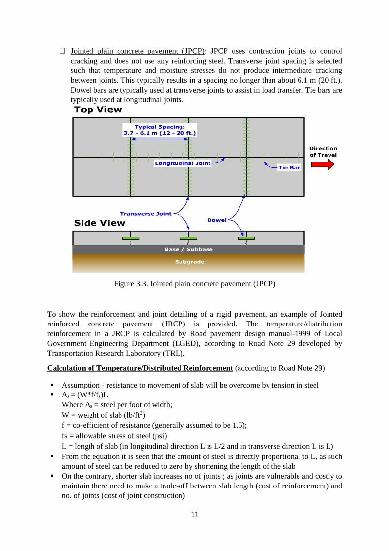
Jointed plain concrete pavement (JPCP): JPCP uses contraction joints to control

cracking and does not use any reinforcing steel. Transverse joint spacing is selected

such that temperature and moisture stresses do not produce intermediate cracking

between joints. This typically results in a spacing no longer than about 6.1 m (20 ft.).

Dowel bars are typically used at transverse joints to assist in load transfer. Tie bars are

typically used at longitudinal joints.

Figure 3.3. Jointed plain concrete pavement (JPCP)

To show the reinforcement and joint detailing of a rigid pavement, an example of Jointed

reinforced concrete pavement (JRCP) is provided. The temperature/distribution

reinforcement in a JRCP is calculated by Road pavement design manual-1999 of Local

Government Engineering Department (LGED), according to Road Note 29 developed by

Transportation Research Laboratory (TRL).

Calculation of Temperature/Distributed Reinforcement (according to Road Note 29)

Assumption - resistance to movement of slab will be overcome by tension in steel

As = (W*f/fs)L

Where As = steel per foot of width;

W = weight of slab (lb/ft2)

f = co-efficient of resistance (generally assumed to be 1.5);

fs = allowable stress of steel (psi)

L = length of slab (in longitudinal direction L is L/2 and in transverse direction L is L)

From the equation it is seen that the amount of steel is directly proportional to L, as such

amount of steel can be reduced to zero by shortening the length of the slab

On the contrary, shorter slab increases no of joints ; as joints are vulnerable and costly to

maintain there need to make a trade-off between slab length (cost of reinforcement) and

no. of joints (cost of joint construction)

12

Selection Criteria of slab length and its type

a. Stabilized sub-base

Cement treated Sub-base/base add to the structural capability of pavement &

also assist in load transfer across joints without dowel bars

therefore, use of short slabs (increase no of joints) and a cement-treated sub-base

sometimes go hand- in hand

b. Plain Versus Reinforced Pavements

Plain pavements:

no temperature reinforcement is required

no contraction joints

dowel bars at expansion joints are also omitted if stabilized sub-base is used

suitable for

o pavements that will carry low volume of traffic and

o slab length is < 6m or 20'

Simply reinforcement pavements:

when slab length lies in between 6m (20') to 23m (75')

it became necessary to use

o some steel for crack control as well as contraction joints

o dowel bars at the joints to assist with load transfer

suitable for pavements that will carry medium volume of traffic

Continuously reinforced pavements

when slab length is > 23m or 75'

amount of steel required to hold the cracks become excessive

no need for contraction joints

13

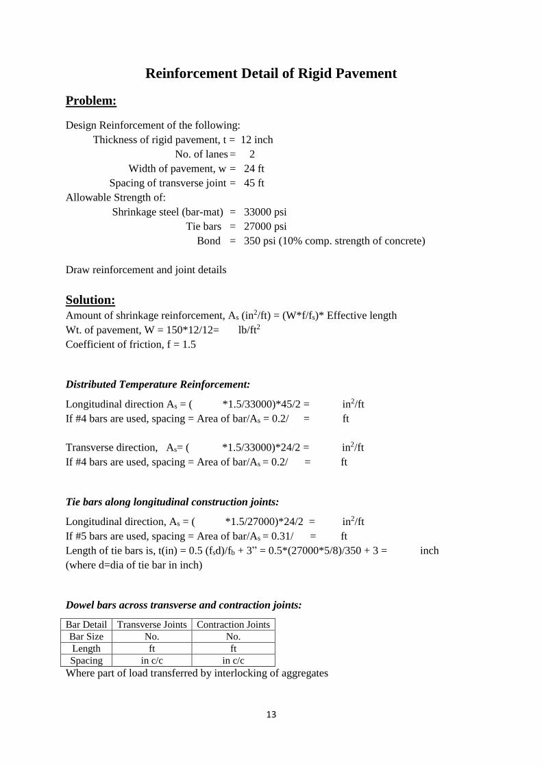
Reinforcement Detail of Rigid Pavement

Problem:

Design Reinforcement of the following:

Thickness of rigid pavement, t = 12 inch

No. of lanes = 2

Width of pavement, w = 24 ft

Spacing of transverse joint = 45 ft

Allowable Strength of:

Shrinkage steel (bar-mat) = 33000 psi

Tie bars = 27000 psi

Bond = 350 psi (10% comp. strength of concrete)

Draw reinforcement and joint details

Solution:

Amount of shrinkage reinforcement, As (in2/ft) = (W*f/fs)* Effective length

Wt. of pavement, W = 150*12/12= lb/ft2

Coefficient of friction, f = 1.5

Distributed Temperature Reinforcement:

Longitudinal direction As = ( *1.5/33000)*45/2 = in2/ft

If #4 bars are used, spacing = Area of bar/As = 0.2/ = ft

Transverse direction, As= ( *1.5/33000)*24/2 = in2/ft

If #4 bars are used, spacing = Area of bar/As = 0.2/ = ft

Tie bars along longitudinal construction joints:

Longitudinal direction, As = ( *1.5/27000)*24/2 = in2/ft

If #5 bars are used, spacing = Area of bar/As = 0.31/ = ft

Length of tie bars is, t(in) = 0.5 (fsd)/fb + 3” = 0.5*(27000*5/8)/350 + 3 = inch

(where d=dia of tie bar in inch)

Dowel bars across transverse and contraction joints:

Bar Detail Transverse Joints Contraction Joints

Bar Size No. No.

Length ft ft

Spacing in c/c in c/c

Where part of load transferred by interlocking of aggregates

14

5. Catalogue Method of Pavement Design

Considering the behavior of local materials, climatic condition and construction practices, a

Catalogue of Pavement Structure is developed

To simplify design procedure

To prevent both under design and over design and thereby

To ensure economical design

The method is designed by LGED (Local Government Engineering Department) as per the

Road Note 31 delivered by TRL (Transportation Research Laboratory) of UK Government.

This design method is applicable for –

Undivided rural road having crest width ranging from 5.6-7.3 m.

Flexible and semi-rigid pavement (i.e. ratio of modulus between two

successive layer is <5)

Cumulative traffic 0.5-3.0 MESA (million equivalent standard axle)

This design method is established based on –

Empirical Analysis – investigating behavior of existing pavement structure

and experience gathered in other countries with similar conditions

Experimental results – laboratory tests of local soil and road construction

materials

Theoretical knowledge – consideration of pavement mechanism i.e. elastic

theory of pavement behavior under the effect of traffic

Finally design catalogue is prepared by checking PADMA (Pavement Design

by Mathematical Analysis) software (stress and strain are calculated at the

interface of the layers and compared with admissible values as function of

expected maximum axle load, cumulative traffic, material characteristics)

Structures proposed are intended to use materials and construction technique

traditionally pertaining in Bangladesh.

A balancing between geometric and structural design of pavement

15

Problem: Design flexible pavement for an undivided rural highway by using catalogue

of pavement structure method for the following data and also determine the

construction of a 10 km highway.

Given:

The forecast AADT for 2003 the year of opening is assessed as:

Vehicle Types Two-way AADT

vpd

Large Truck 450

Small Truck 90 Assume:

Large Bus 400 Growth Rate, r = 7.5% per annum

Small Bus 30 Design Period, n = 15 year

Car 200 CBR of Subgrade = 9.0%

Autorickshaw 50

Motocycle 30

Bicycle 50

Rickshaw 60

Cart 10

Solution:

(A) Determination of Roadway Geometry

Vehicle Types Two-way

AADT

vpd

PCU Factors PCU/day at

2003

Large Truck

Small Truck

Large Bus

Small Bus

Car

Autorickshaw

Motocycle

Bicycle

Rickshaw

Cart

Total =

16

Forecasted design flow in 2018 = Total PCU/day at 2003 X (1+ growth rate) (design period)

= X (1.075)15 PCU/day

From the manuals of geometric design standards the recommended:

Road Width = m

Shoulder Width = m

(B) Determination of Cumulative ESAL for Pavement Design

Heavy Vehicle

Types

Two-way AADT

vpd

ESAL per

vehicle

Cumulative

ESAL*

Large Truck

Small Truck

Large Bus

Small Bus

Total =

*Cumulative ESAL = 365 x AADT x ESAL x [(1+r)n−1]

r

Total Cumulative ESAL in both direction =

Total Cumulative ESAL in one direction = DD= 50.0%

Determination of Channelization Factor

The proportion of non-motorized traffic to heavy vehicle is:

P = ( + + )/( + + + ) =

By interpolation Channelization factor from table 3 =

Design Cumulative Traffic =

=

ESA

MSA

( C ) Determination of Pavement Layer Thickness

Traffic Class =

for MSA

Subgrade Class =

for 9% CBR

Using charts for catalogue propose alternative designs of pavement with varying material

types. Then evaluate alternatives based on availability of materials, construction strategy and

economy.

17

Table 1: PCU factors for rural road

Table 2: ESAL per vehicle

Vehicle Types PCU factors

Vehicle Types

ESAL per

veh.

Large Truck 3.0

Large Truck 1.5

Small Truck 2.0

Smsll Truck 0.5

Large Bus 2.5

Large Bus 0.5

Small Bus 1.5

Small Bus 0.2

Car 1.0

Autorickshaw 0.8

Motorcycle 0.5

Bicycle 0.3

Rickshaw 2.0

Other 4.0

Table 3: Channelization Factor

Road Width

Channelization factor depending on the

ratio of NMV to be applied to one way

flow

m ft Low

(<0.5) High ( >= 0.5)

5.6 18.4 2.0 2.0

6.8 22.3 1.0 1.8

7.3 23.9 1.0 1.6

Table 4: Traffic Definition

Table 5: Subgrade Definition

Class MSA

Class CBR

T0 < 0.5

S1 3-5

T1 0.5-1.5

S2 5-7

T2 1.5-3.0

S3 7-10

T3 3.0-7.5

S4 10-15

T4 7.5-20.0

S5 >15

T5 20.0-30.0

18

6. Airport Pavement Design

SCOPE

All the methodology, charts and table presented below are as per AC 150/5320-6D of Federal

Aviation Administration (FAA) of US Department of Transportation (DoT). This method

covers pavement design for airports serving aircraft with gross weights of 30,000 pounds

(13 000 kg) or more.

BACKGROUND

An airfield pavement and the operating aircraft represent an interactive system which must be

addressed in the pavement design process. Design considerations associated with both the

aircraft and the pavement must be recognized in order to produce a satisfactory design.

Careful construction control and some degree of maintenance will be required to produce a

pavement which will achieve the intended design life. Pavements are designed to provide a

finite life and fatigue limits are anticipated. Poor construction and lack of preventative

maintenance will usually shorten the service life of even the best designed pavement.

a. Variables.

The determination of pavement thickness requirements is a complex engineering problem.

Pavements are subject to a wide variety of loadings and climatic effects. The design process

involves a large number of interacting variables which are often difficult to quantify.

Although a great deal of research work has been completed and more is underway, it has

been impossible to arrive at a direct mathematical solution of thickness requirements. For this

reason the determination of pavement thickness must be based on the theoretical analysis of

load distribution through pavements and soils, the analysis of experimental pavement data,

and a study of the performance of pavements under actual service conditions. Pavement

thickness curves presented here have been developed through correlation of the data obtained

from these sources. Pavements designed in accordance with these standards are intended to

provide a structural life of 20 years that is free of major maintenance if no major changes in

forecast traffic are encountered. It is likely that rehabilitation of surface grades and renewal

of skid resistant properties will be needed before 20 years due to destructive climatic effects

and deteriorating effects of normal usage.

b. Structural Design

The structural design of airport pavements consists of determining both the overall pavement

thickness and the thickness of the component parts of the pavement. There are a number of

factors which influence the thickness of pavement required to provide satisfactory service.

These include the magnitude and character of the aircraft loads to be supported, the volume

of traffic, the concentration of traffic in certain areas, and the quality of the subgrade soil and

materials comprising the pavement structure.

19

AIRCRAFT CONSIDERATIONS

a. Load

The pavement design method is based on the gross weight of the aircraft. For design purposes

the pavement should be designed for the maximum anticipated takeoff weight of the aircraft.

The design procedure assumes 95 percent of the gross weight is carried by the main landing

gears and 5 percent is carried by the nose gear. AC 150/5300-13, Airport Design, lists the

weight of nearly all civil aircraft. Use of the maximum anticipated takeoff weight is

recommended to provide some degree of conservatism in the design and is justified by the

fact that changes in operational use can often occur and recognition of the fact that forecast

traffic is approximate at best. By ignoring arriving traffic some of the conservatism is offset.

b. Landing Gear Type and Geometry

The gear type and configuration dictate how the aircraft weight is distributed to the pavement

and determine pavement response to aircraft loadings. It would have been impractical to

develop design curves for each type of aircraft. However, since the thickness of both rigid

and flexible pavements is dependent upon the gear dimensions and the type of gear, separate

design curves would be necessary unless some valid assumptions could be made to reduce the

number of variables. Examination of gear configuration, tire contact areas, and tire pressure

in common use indicated that these follow a definite trend related to aircraft gross weight.

Reasonable assumptions could therefore be made and design curves constructed from the

assumed data. These assumed data are as follows:

(1) Single Gear Aircraft: No special assumptions needed.

(2) Dual Gear Aircraft: A study of the spacing between dual wheels for these aircraft

indicated that a dimension of 20 inches (0.5 1 m) between the centerline of the tires

appeared reasonable for the lighter aircraft and a dimension of 34 inches (0.86 m)

between the centerline of the tires appeared reasonable for the heavier aircraft.

(3) Dual Tandem Gear Aircraft: The study indicated a dual wheel spacing of 20 inches

(0.51m) and a tandem spacing of 45 inches (1.14 m) for lighter aircraft, and a dual

wheel spacing of 30 inches (0.76 m) and a tandem spacing of 55 inches (1.40 m) for

the heavier aircraft are appropriate design values.

(4) Wide Body Aircraft: Wide body aircraft; i.e., B-747, DC-l0, and L-1011 represent a

radical departure from the geometry assumed for dual tandem aircraft described in

paragraph above. Due to the large differences in gross weights and gear geometries,

separate design curves have been prepared for the wide body aircraft.

c. Tire Pressure

Tire pressure varies between 75 and 200 PSI (516 to 1380 kPa) depending on gear

configuration and gross weight. It should be noted that tire pressure asserts less influence on

pavement stresses as gross weight increases, and the assumed maximum of 200 PSI (1380

kPa) may be safely exceeded if other parameters are not exceeded and a high stability surface

course is used.

d. Traffic Volume

Forecasts of annual departures by aircraft type are needed for pavement design.

20

Information on aircraft operations is available from Airport Master Plans, Terminal Area

Forecasts, and the National Plan of Integrated Airport Systems.

DETERMINATION OF DESIGN AIRCRAFT

The forecast of annual departures by aircraft type will result in a list of a number of different

aircraft. The design aircraft should be selected on the basis of the one requiring the greatest

pavement thickness. Each aircraft type in the forecast should be checked to determine the

pavement thickness required by using the appropriate design curve with the forecast number

of annual departures for that aircraft. The aircraft type which produces the greatest pavement

thickness is the design aircraft. The design aircraft is not necessarily the heaviest aircraft in

the forecast.

DETERMINATION OF EQUIVALENT ANNUAL DEPARTURES BY THE DESIGN

AIRCRAFT

a. Conversions

Since the traffic forecast is a mixture of a variety of aircraft having different landing gear

types and different weights, the effects of all traffic must be accounted for in terms of the

design aircraft. First, all aircraft must be converted to the same landing gear type as the

design aircraft. Factors have been established to accomplish this conversion. These factors

are constant and apply to both flexible and rigid pavements. They represent an approximation

of the relative fatigue effects of different gear types. Much more precise and theoretically

rigorous factors could be developed for different types and thicknesses of pavement.

However, such precision would be impractical for hand calculation as numerous iterations

and adjustments would be required as the design evolved. At this stage of the design process

such precision is not warranted. The following conversion factors should be used to convert

from one landing gear type to another:

Table 6.1: Airport Landing Gear-Configuration Conversion Factors

To Convert from To Multiply Departures by

Single wheel Dual wheel 0.8

Single wheel Dual tandem 0.5

Dual wheel Dual tandem 0.6

Double dual tandem Dual tandem 1.0

Dual tandem Single wheel 2.0

Dual tandem Dual wheel 1.7

Dual wheel Single wheel 1.3

Double dual tandem Dual wheel 1.7

Source: Federal Aviation Administration

Secondly, after the aircraft have been grouped into the same landing gear configuration, the

conversion to equivalent annual departures of the design aircraft should be determined by the

following formula:

log R1= log R2*(W2/W1)1/2

where

R1 =equivalent annual departures by the design aircraft

21

R2=annual departures expressed in design aircraft landing gear

W1=wheel load of the design aircraft

W2=wheel load of the aircraft in question

For this computation 95 percent of the gross weight of the aircraft is assumed to be carried by

the main landing gears.

Wide body aircraft require special attention in this calculation. The procedure discussed

above is a relative rating which compares different aircraft to a common design aircraft.

Since wide body aircraft have significantly different landing gear assembly spacings than

other aircraft, special considerations are needed to maintain the relative effects. This is done

by treating each wide body as a 300,000-pound (136100 kg) dual tandem aircraft when

computing equivalent annual departures. This should be done in every instance even when

the design aircraft is a wide body. After the equivalent annual departures are determined, the

design should proceed using the appropriate design curve for the design aircraft.

For example if a wide body is the design aircraft, all equivalent departures should be

calculated as described above; then the design curve for the wide body should be used with

the calculated equivalent annual departures.

b. Example:

Assume an airport pavement is to be designed for the following forecast traffic:

Aircraft Gear Type Average Annual

Departures

Maximum Takeoff Weight

Lbs. (kg)

727-100 Dual 3760 160,000 (72600)

727-200 Dual 9080 190,500 (86500)

707-320B Dual tandem 3050 327,000 (148500)

DC-g-30 Dual 5800 108,000 (49000)

cv-880 Dual tandem 400 184,500 (83948)

737-200 Dual 2650 115,500 (52440)

L-101 I-100 Dual tandem 1710 450,000 (204120)

747-100 Double dual

tandem

85 700,000 (317800)

(1) Determine Design Aircraft: A pavement thickness is determined for each aircraft in the

forecast using the appropriate design curves. The pavement input data, CBR, K value,

flexural strength, etc., should be the same for all aircraft. Aircraft weights and departure

levels must correspond to the particular aircraft in the forecast.

In this example the 727-200 requires the greatest pavement thickness and is thus the design

aircraft.

(2) Group Forecast Traffic into Landing Gear of Design Aircraft: In this example the

design aircraft is equipped with a dual wheel landing gear so all traffic must be grouped into

the dual wheel configuration.

22

(3) Convert Aircraft to Equivalent Annual Departures of the Design Aircraft: After the

aircraft mixture has been grouped into a common landing gear configuration, the equivalent

annual departures of the design aircraft can be calculated.

Aircraft Equivalent

Dual Gear

Departures

Wheel load Wheel load of design

aircraft

Equivalent

Annual Departs

Design Aircraft lbs (kg)

Lbs (kg)

727-100 3760 38000 (17240) 45240 (20520) 1891

727-200 9080 45240 (20520) 45240 (20520) 9080

707-320B 5185 38830 (17610) 45240 (20520) 2764

DC-g-30 5800 25650 (11630) 45240 (20520) 682

cv-880 680 21910 (9940) 45240 (20520) 94

737-200 2650 27430 (12440) 45240 (20520) 463

L-101 I-100 145 35625* (16160) 45240 (20520) 83

747-100 2907 35625* (16160) 45240 (20520) 1184

Total= 16241

(4) Final Result: For this example the pavement would be designed for 16,000 annual

departures of a dual wheel aircraft weighing 190,500 pounds (86 500 kg). The design should,

however, provide for the heaviest aircraft in the traffic mixture, B747-100, when considering

depth of compaction, thickness of asphalt surface, drainage structures, etc.

23

Problem

Design a flexible pavement for airport using FAA method for following data:

Forecast Aircraft Traffic Data for a Typical Airport

Aircraft Type Forecast Annual

Departures

Main Landing Gear

Configuration

Gross Take-off

Weight, kip

B-727-100 3,000 Dual 160

B-727-200 4,000 Dual 185

B-707-320B 3,000 Dual tandem 327

CV-880 1,000 Dual tandem 185

DC-9-30 1,200 Dual 108

B-737-200 900 Dual 100

L-1011-100 1,300 Dual tandem 510

B-747-100 1,200 Double dual tandem 710

A-340-200 1,000 Dual tandem & Dual 559

Design Pavement Life = 20 years

24

Solution:

A. Determination of Design Aircraft

Thickness requirement for each aircraft is determined by using design curves (Fig- 1 to Fig-

14, Appendix 1), considering same input data (CBR, k value etc) for all aircraft. Gross

weights and no. of departures must correspond to the particular aircraft in the forecast list.

Design Aircraft1 Data

Aircraft Type

Gear Type

Gross Wt, Wg (kip)

Wheel Load, W1 (kip)

B. Determination of Equivalent Departures of Design Aircraft

Aircraft

Type

Forecast

Annual

Departure

s (R)

Gross Wt.

on main

landing

gears (W2)

Total

No. of

wheels3

Load/

Wheel

(W2)4

Gear

Conversion

Factor,

GCF5

Equivalent Departures

of

Design

Gear (R2)5

Design

Wheel

Load (R1)7

B-727-100 3,000

B-727-200 4,000

B-707-320B 3,000

CV-880 1,000

DC-9-30 1,200

B-737-200 900

L-1011-100 1,300

B-747-100 1,200

A-340-200 1,000

Total Equivalent Annual Departures of Design Aircraft=

___________________________________________________________________________

Notes:

1. The aircraft which requires greatest pavement thickness

2. 95% of the gross take-off weight is assumed to be carried by the main landing gears.

Wide body aircraft is considered as a 300 kip Dual tandem aircraft

3. See Fig 6.1: Landing Gear Configuration

4. Load per wheel= W/Total no. of wheels

5. For Gear Conversion Factor (GCF) see Table 6.1

6. R2= R*GCF

25

Design Aircraft Data Design CBR Values

Aircraft Type Subgrade 5

Gear Type Subbase 20

Gross gear wt. (kip)

Total Equivalent Departures

Determination of Pavement Layer Thicknesses for Critical Areas

Thicknesses from the appropriate design curve Inputs/Calculations inch

T1= Total thickness above subgrade (i.e. Surface+Base+Subbase) App 2, Fig: 2 ; CBR= 5

T2= Total thickness above subase (i.e. Surface+Base) App 2, Fig: 2 ; CBR= 20

T3= Minimum thickness of untreated base course

T4= Minimum thickness of Surface course App 2, Fig: 2 Calculated Thickness of Base and Subbase Course

T5= thickness of untreated subbase T1-T2

T6= thickness of untreated base course T2-T4

Check for minimum base course As T6<T3, use T3 instead of T6

Adjusted base and subbase course thicknesses

T7= Due to minimum criterion, the extra thickness of base course

would be T7

This extra thickness need be deducted from the subbase thickness,

T5 instead of adding with the total pavement thickness, T1

T3-T6

T8= So the pavement thickness becomes T8 T5-T7

Stabilized Subbase and Base Courses

As the design aircraft Wt.>100 kip, stabilized subbase/base needs to

be used

If soil cement base course materials are used for subbase stabilization then

the thickness of stabilized subbase would be

App 3, Table:1

T8/Stabilization Factor

If cement base course materials are used for base stabilization then the

thickness of stabilized base would be App 3, Table:1

T3/Stabilization Factor

Thicknesses for Non-critical areas

Surface Course

The minimum thickness of stabilized base would be

App 2; Fig:2

Base and Subbase Courses

At high speed areas: The thickness of subbase course would be

The thickness of base course would be

0.9 of Critical Thickness

0.9 of Critical Thickness

At pavement edges: The thickness of base would be 0.7 of critical thickness

The subbase is not reduced to allow for transverse drainage.

The final design thickness would be as follows

Pavement Layer

Thickness requirements (rounded to even increments)

Critical Areas (in) Non-critical (in)

High Speed Areas Pavement Edges

Bituminous Surface

Base Course

Subbase Course

26

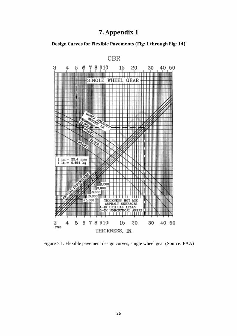
7. Appendix 1

Design Curves for Flexible Pavements (Fig: 1 through Fig: 14)

Figure 7.1. Flexible pavement design curves, single wheel gear (Source: FAA)

27

Figure 7.2. Flexible pavement design curves, dual wheel gear (Source: FAA)

28

Figure 7.3. Flexible pavement design curves, dual tandem gear (Source: FAA)

29

Figure 7.4. Flexible pavement design curves, a-300 model b2 (Source: FAA)

30

Figure 7.5. Flexible pavement design curves, a-300 model b4 (Source: FAA)

31

Figure 7.6. Flexible pavement design curves, b-747-loo, sr, 200 b, c, f (Source: FAA)

32

Figure 7.7. Flexible pavement design curves, b-747-sp (Source: FAA)

33

Figure 7.8. Flexible pavement design curves, B-757 (Source: FAA)

34

Figure 7.9. Flexible pavement design curves, B-767 (Source: FAA)

35

Figure 7.10. Flexible pavement design curves, C-130 (Source: FAA)

36

Figure 7.11. Flexible pavement design curves, DC 10-10, 1OCF (Source: FAA)

37

Figure 7.12. Flexible pavement design curves, DC 10-30,30CF, 40,40CF (Source: FAA)

38

Figure 7.13. Flexible pavement design curves, L-1011-1,100 (Source: FAA)

39

Figure 7.14. Flexible pavement design curves, L-1011-1,200 (Source: FAA)

40

8. Appendix 2

Table 1: Recommended Equivalent Factors for Stabilized Subbase Course

Material Used Equivalency Factor

Subbase Base

Bituminous Surface Course 1.7-2.3 1.2-1.6

Bituminous base course 1.7-2.3 1.2-1.6

Cold laid bituminous base course 1.5-1.7 1.0-1.2

Mixed in-place base course 1.5-1.7 1.0-1.2

Cement treated base course 1.6-2.3 1.2-1.6

Soil cement base course 1.5-2.0 N/A

Crushed aggregate base course 1.4-2.0 1

Gravel subbase course 1 N/A

41

9. Reference

1. Local Government Engineering Division, 2003. Road Pavement Design Manual.

2. Road Note 29 by Transportation Research Laboratory (TRL)

3. AC 150/5320-6D, Federal Aviation Administration (FAA) of US Department of

Transportation (DoT)