Cars, carbon taxes and CO2 emissions

Julius Andersson

October 2015

Centre for Climate Change Economics and Policy

Working Paper No. 238

Grantham Research Institute on Climate Change and

the Environment

Working Paper No. 212

The Centre for Climate Change Economics and Policy (CCCEP) was established by the University of Leeds and the London School of Economics and Political Science in 2008 to advance public and private action on climate change through innovative, rigorous research. The Centre is funded by the UK Economic and Social Research Council. Its second phase started in 2013 and there are five integrated research themes:

1. Understanding green growth and climate-compatible development 2. Advancing climate finance and investment 3. Evaluating the performance of climate policies 4. Managing climate risks and uncertainties and strengthening climate services 5. Enabling rapid transitions in mitigation and adaptation

More information about the Centre for Climate Change Economics and Policy can be found at: http://www.cccep.ac.uk. The Grantham Research Institute on Climate Change and the Environment was established by the London School of Economics and Political Science in 2008 to bring together international expertise on economics, finance, geography, the environment, international development and political economy to create a world-leading centre for policy-relevant research and training. The Institute is funded by the Grantham Foundation for the Protection of the Environment and the Global Green Growth Institute. It has nine research programmes:

1. Adaptation and development 2. Carbon trading and finance 3. Ecosystems, resources and the natural environment 4. Energy, technology and trade 5. Future generations and social justice 6. Growth and the economy 7. International environmental negotiations 8. Modelling and decision making 9. Private sector adaptation, risk and insurance

More information about the Grantham Research Institute on Climate Change and the Environment can be found at: http://www.lse.ac.uk/grantham. This working paper is intended to stimulate discussion within the research community and among users of research, and its content may have been submitted for publication in academic journals. It has been reviewed by at least one internal referee before publication. The views expressed in this paper represent those of the author(s) and do not necessarily represent those of the host institutions or funders.

Cars, Carbon Taxes and CO2 Emissions

Julius J. Andersson*

Department of Geography and Environment

Grantham Research Institute on Climate Change and the Environment

ESRC Centre for Climate Change Economics and Policy

London School of Economics and Political Science, UK

October, 2015

Abstract: Is a carbon tax effective in reducing emissions of greenhouse gases, and thereby

mitigating climate change? I estimate the reduction in emissions of carbon dioxide (CO2) from

the transport sector in Sweden during the years 1990 to 2005 as a result of the introduction of a

carbon tax and a value added tax (VAT) on transport fuel in the years 1990-1991. To capture the

causal effect on emissions I construct a synthetic Sweden, the counterfactual Sweden that does

not receive the ‘treatment’ in 1990-1991, using the synthetic control method. The results show a

reduction in emissions of 10.9% during the post-treatment period of 1990-2005, equivalent to

2.5 million metric tons of CO2 in the annual total. Looking at the effect of the carbon tax in

isolation I estimate a post-treatment reduction of 4.9%, equivalent to 1.1 million metric tons of

CO2 in an average year. The results are robust to a series of placebo tests, both in-time and in-

space. Taken together, my findings show that a carbon tax can be an efficient tool to mitigate

climate change.

JEL-classification: Q58, H23

Keywords: Carbon tax, transport sector, synthetic control method, climate change

*Contact: j.j.andersson@lse.ac.uk. I would like to thank Jared Finnegan, Dominik Hangartner and Sara Hellgren for

helpful thoughts, comments and discussions. Any errors in this paper are my own. I am grateful to the London School of Economics for financial support. Support was also received from the Grantham Foundation for the Protection of the Environment and the ESRC Centre for Climate Change Economics and Policy.

2

1. Introduction

In this paper I provide an estimate of the reduction in emissions of carbon dioxide (CO2) from

1990 to 2005 in the Swedish transport sector as a result of the introduction of a carbon tax and a

value added tax (VAT) on transport fuel in the years 1990-1991. I first construct synthetic

Sweden, the counterfactual Sweden that does not receive the ‘treatment’ (i.e., the carbon tax and

VAT), using the synthetic control method (Abadie and Gardeazabal 2003; Abadie, Diamond,

and Hainmueller 2010; 2014). Secondly, I estimate the difference in emissions between Sweden

and synthetic Sweden and analyse how robust the results are by performing a series of placebo

tests. Lastly, I try to disentangle the effect of the carbon tax and the VAT from each other. My

results show that the policy changes of introducing a carbon tax and VAT in 1990-1991 had a

significant effect on CO2 emissions from the transport sector.

In 1991 Sweden was one of the first countries in the world to introduce a carbon tax.

The tax level was initially set at 250 SEK ($30) per ton of CO2 and then successively raised to the

current level of 1100 SEK ($132). The goal of the tax is to reduce emissions of CO2, the main

greenhouse gas (GHG) contributing to climate change, by equalizing the private and social cost

of carbon. In the year prior, in March of 1990, Sweden also added VAT of 25% to the price of

gasoline and diesel. The VAT is applied to both the underlying cost of the transport fuel and any

added energy and/or carbon taxes.

Although the carbon tax was implemented quite broadly, some sectors of the economy,

especially industry and agriculture received a lower rate in 1993 and onwards due to competitive

concerns, and some high-energy sectors, such as mining and the pulp and paper industry, are

fully exempted from paying the tax. Consequently, when evaluating the environmental efficiency

of the tax it is not advisable to look at total CO2 emissions in Sweden since many units in the

economy do not receive the treatment.1 Fortunately, the transport sector, the largest source of

CO2 emissions in Sweden, is fully covered by the carbon tax and thus a suitable sector to analyse.

From 1990 to 2005 the sector was responsible for close to 40% of Sweden’s annual CO2

emissions.

An advantage of focusing solely on transport is that the risk of carbon leakage – firms

reallocating to countries without strict climate change policies – is arguably smaller for this sector

compared to, for instance, manufacturing and energy production. If a carbon tax in country X

leads to carbon leakage and increase of emissions in country Z, we have interference between

1 Two underlying assumptions in analyses of causal effects are (1) no interference between units, and that (2) all

treated units receive the same dose of the treatment. If total CO2 emissions are the dependent variable in our analysis, then clearly assumption (2) is violated.

3

units. An analysis of country X would thus overestimate the effect on emissions from the carbon

tax. Transportation of goods and people, however, still needs to be done within a country’s

borders and cannot easily be outsourced.

From 1990 to 2007, GHG emissions in Sweden decreased by 9% while GDP grew by

48% (Ministry of the Environment and Energy 2009). One may be tempted to put forward this

as evidence that the carbon tax has been successful. The problem is that these emissions

reductions cannot be taken as evidence of the causal effect of the tax since we have no

counterfactual to compare with. This is the fundamental problem of causal inference: we cannot

observe the outcome under treatment and the outcome when not treated, for the same unit

(Holland 1986). To address this problem I make use of the synthetic control method, which

allows me to create the missing counterfactual as a synthetic Sweden, consisting of a weighted

combination of suitable ‘donor’ countries that did not implement carbon taxation, or other

similar policy changes, but that had similar pre-treatment trajectories of CO2 emissions in the

transport sector.

This study is one of the few ex-post empirical studies that estimate the causal effect on

emissions from carbon taxation. Sweden, together with Denmark, Finland, Norway and the

Netherlands, were the first countries to implement carbon taxes, and did so in the early 1990s.

However, almost all studies of the environmental impact of these taxes are ex-ante simulations

and very few are ex-post empirical studies (Andersen et al. 2001; Baranzini & Carattini 2013).

This lack of ex-post empirical studies is likely due to methodological difficulties, specifically the

issue that “no base-line scenario without the tax exists for purposes of comparison” (Bohlin

1998, p. 283). This issue is precisely what the synthetic control method seeks to overcome. The

few ex-post studies that do exist all find that carbon taxes have had either no impact (Lin & Li

2011; Bohlin 1998) or a fairly small impact on CO2 emissions. For example, Brunvoll and Larsen

(2004) find a 2% reduction in Norwegian CO2 emissions as a result of that country’s carbon tax.

Contrary to these studies, I find transport CO2 emissions in Sweden to be 12.5%, or 3.2 million

metric tons, lower in 2005 than they would have otherwise been in the absence of the policy

changes. The reduction in emissions for the 1990-2005 period is 10.9%, or 2.5 million metric

tons of CO2 in an average year. And from the carbon tax alone I estimate a post-treatment

reduction of 4.9%.

2. Method and Data

To assess the carbon tax in Sweden, I first construct the missing counterfactual using a weighted

combination of other OECD countries that resemble Sweden on a number of key predictors for

4

CO2 emissions in transport prior to treatment. This particular method of constructing the

counterfactual, called the synthetic control method, is developed and described in Abadie and

Gardezabal (2003) and Abadie, Diamond, and Hainmueller (2010; 2014)2.

Let 𝐽 + 1 be the number of OECD countries in my sample, indexed by 𝑗, and let 𝑗 = 1

denote Sweden, the “treated unit”. The units in the sample are observed for time periods

𝑡 = 1, 2, … , 𝑇. It is important to have data on a sufficient amount of time periods prior to

treatment 1, 2, … , 𝑇0 and post treatment 𝑇0 + 1, 𝑇0 + 2, … , 𝑇 to be able to both construct a

synthetic Sweden and evaluate the effect of the treatment.

Next we define two potential outcomes: 𝑌𝑗𝑡𝐼 refers to CO2 emissions from transport when

exposed to treatment for unit 𝑗 at time 𝑡 and 𝑌𝑗𝑡𝑁 is CO2 emissions without treatment. The goal

of the analysis is to measure the post-treatment effect on emissions in Sweden, which can be

formalised as 𝛼1𝑡 = 𝑌1𝑡𝐼 − 𝑌1𝑡

𝑁. However, since we cannot observe 𝑌1𝑡𝑁 in the post-treatment

period we need to construct it using synthetic control.

Synthetic Sweden is constructed as a weighted average of control countries 𝑗 = 2, … , 𝐽 +

1 from my donor pool of OECD countries, and represented by a vector of weights 𝑊 =

(𝑤2, … , 𝑤𝐽+1)′ with 0 ≤ 𝑤𝑗 ≤ 1 and 𝑤2 + ∙ ∙ ∙ +𝑤𝐽+1 = 1. Each choice of 𝑊gives a certain set

of weights and hence characterises a possible synthetic control. We want the synthetic control to

not only be able to reproduce the trajectory of CO2 emissions but also to be similar to Sweden

on a number of pre-treatment predictors of the outcome variable. Hence, let 𝑍𝑗 denote the

vector of observed predictors for each unit in the sample. Now suppose that we find 𝑊 =

𝑊∗ = (𝑤2∗, … , 𝑤𝐽+1

∗ ) such that for the pre-treatment period 𝑡 ≤ 𝑇0 we have that

∑ 𝑤𝑗∗𝑌𝑗1 = 𝑌11, ∑ 𝑤𝑗

∗𝑌𝑗2 = 𝑌12

𝐽+1

𝑗=2

, ⋯ , ∑ 𝑤𝑗∗𝑌𝑗𝑇0

= 𝑌1𝑇0,

𝐽+1

𝑗=2

𝐽+1

𝑗=2

and ∑ 𝑤𝑗∗𝑍𝑗 = 𝑍1

𝐽+1

𝑗=2

then, as proved in Abadie et al. (2010), for the post-treatment period 𝑇0 + 1, 𝑇0 + 2, … , 𝑇 we

can use the following as an unbiased estimator of 𝛼1𝑡:

�̂�1𝑡 = 𝑌1𝑡 − ∑ 𝑤𝑗∗𝑌𝑗𝑡

𝐽+1

𝑗=2

2 The description here follows the structure in Abadie, Diamond, and Hainmueller (2010; 2011).

5

To find 𝑊∗ we need to define a measurable distance between Sweden and its control

units which we then minimize. Let 𝑋1 = (𝑍1′ , 𝑌11, … , 𝑌1𝑇0

)′ denote an (𝑘 x 1) vector of pre-

treatment values for the key predictors of the outcome variable and the outcome variable itself

for Sweden, and let the (𝑘 x 𝐽) matrix 𝑋0 contain similar variables for the control countries.3 We

then choose 𝑊∗ so that the distance ‖𝑋1 − 𝑋0𝑊‖ is minimized for the pre-treatment period,

subject to the above (convexity) constraints on the weights. In this paper I solve for a 𝑊∗ that

minimizes:

‖𝑋1 − 𝑋0𝑊‖𝑣 = √(𝑋1 − 𝑋0𝑊)′𝑉(𝑋1 − 𝑋0𝑊)

where 𝑉 here is the (𝑘 x 𝑘) symmetric and positive semidefinite matrix that minimizes the mean

squared prediction error (MSPE) of the outcome variable over the entire pre-treatment period.4

The purpose of introducing 𝑉 is to weight the predictors and allow more weight being

given to more important predictors of the outcome variable. Here, 𝑉 is chosen through a data-

driven procedure but other methods are possible, for instance, assigning weights to the

predictors based on empirical findings in the literature on the main drivers of CO2 emissions, or

cross-validation methods (Abadie et al. 2014).

2.1 Data

I use annual panel data on CO2 emissions from transport for the years 1960-2005 for 24 OECD

countries (including Sweden). I chose 2005 as the end date because that year was the start of the

EU Emissions Trading System (EU ETS), one of the main building blocks of the EU’s climate

change policy, and also because many countries in the sample implemented carbon taxes or

made marked changes to fuel taxation from 2005 and onwards. The sample period hence gives

me thirty years of pre-treatment data and sixteen years of post-treatment data, which should be

enough to both construct a viable synthetic Sweden and enough time post-treatment to evaluate

the effect of the policy changes.

From this initial sample of donor countries I exclude countries that during the sample

period enacted carbon taxes that cover the transport sector, in this case: Finland, Norway, and

the Netherlands, or made large changes to fuel taxes, which exclude Germany, Italy, and the

3 Note that the main analysis does not use all pre-treatment values for the outcome variable, only values for three

distinct years. 4 To find 𝑉(which here is diagonal) and 𝑊∗ I used a statistical package for R called Synth (Abadie et al. 2011).

6

UK.5 Additionally, I exclude Austria and Luxembourg due to “fuel tourism” skewing their

emissions data. Austria’s emissions data is skewed from the year 1999 and onwards. This is due

to Austria lowering fuel taxes in 1999, while neighbouring Germany and Italy increased their fuel

taxes the same year. Austria is a major transit country and large trucks in particular tend to fill up

in countries with low diesel prices on their way through Europe. In 2005, diesel sales in Austria

where 150% higher than a decade earlier, a clear indication that “fuel tourism” had taken place.

Luxembourg has had lower fuel taxes than neighbouring European countries for many years,

which explains them having five to eight times higher per capita consumption of fuel than their

neighbours (European Federation for Transport and Environment 2011) and more than two

times higher CO2 emissions from transport than the next highest emitter in the sample. Lastly, I

exclude Ireland due to their unique “Celtic Tiger” economic expansion in the 1990s which more

than doubled both their GDP per capita and CO2 emissions per capita from transport during the

post-treatment period. This rapid economic expansion is very dissimilar to Sweden’s and the

other donor countries’ development during the same time period.6 In the end, my donor pool

consists of 14 countries: Australia, Belgium, Canada, Denmark, France, Greece, Iceland, Japan,

New Zealand, Poland, Portugal, Spain, Switzerland, and the United States.

The outcome variable is per capita CO2 emissions from transport and measured in metric

tons. The data, obtained from the World Bank, contains emissions from the combustion of fuel

from road, rail, domestic navigation, and domestic aviation, excluding international aviation and

international marine bunkers. As key predictors I use GDP per capita, number of motor vehicles

(per 1000 people), gasoline consumption per capita, and percentage of urban population (see

Appendix for details and sources). The level of GDP per capita is shown in the literature to be

closely linked to emissions of greenhouse gases (Neumayer, 2004), and OECD countries that are

less urbanized have a higher usage of motor vehicles and hence higher emissions from transport.

I average the four key predictors over the 1980-1989 period. Finally, to the list of predictors I

add three lagged years of CO2 emissions: 1970, 1980, and 1989.

5 Denmark also implemented a carbon tax, in 1992. However, their tax level is set very low and, more importantly,

the transport sector is exempted. 6 Note that including Austria and Ireland in the donor pool does not change the main results in this paper since they

both receive zero weights in synthetic Sweden.

7

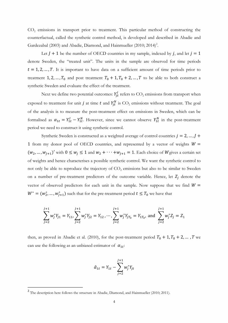
Figure 1. Trajectory of CO2 emissions from transport in Sweden vs. the OECD average of my 14 donor countries.

Figure 1 shows the trajectory of emissions from transport in Sweden and the OECD

average during the sample period7. The fit is particularly poor for the ten years prior to the

introduction of the carbon tax and VAT. Next, in the results section, I show how the synthetic

control method is able to provide a synthetic Sweden with a much better fit on emissions for the

pre-treatment period. This thus gives us a more reliable way to estimate the causal effect on

emissions as a result of the policy changes.

7 The slump in emissions in Sweden and the OECD countries in the years following 1979 is a response to what is

commonly called the “second oil crisis”, prompted by the Iranian Revolution in 1979. It wasn’t until around 1986

that the price of oil was back down at pre-1979 levels. This increase in the oil price hence acts as a ‘natural

experiment’ that shows that increased prices of fuel leads to reductions in CO2 emissions from transport.

1960 1970 1980 1990 2000

0.0

0.5

1.0

1.5

2.0

2.5

3.0

Year

Metr

ic ton

s p

er

ca

pita (

CO

2 fro

m tra

nsp

ort

)

SwedenOECD sample

VAT + Carbon tax

8

3. Results and Robustness Check

First, I analyse if synthetic Sweden is able to track the CO2 emissions from transport in Sweden

for the pre-treatment period and how closely it reproduces the values of the key predictors. A

good fit is important to lend credibility to our identification assumption, which asserts that

synthetic Sweden shows the trajectory of CO2 emissions from transport in Sweden from 1990 to

2005 had the policy changes of introducing VAT and a carbon tax not taken place.

Figure 2 shows that, prior to treatment, CO2 emissions from transport in synthetic Sweden

track actual emissions in Sweden very closely. The average (absolute) difference for the pre-

treatment period is only around 0.03 metric tons of CO2 (or 1.79%).

Table 1 compares the values of the key predictors for Sweden prior to 1990 with the same

values for synthetic Sweden and a population-weighted average of the 14 OECD countries in the

donor pool. For all predictors except gasoline consumption per capita, Sweden and synthetic

Sweden have very similar values and a much better fit compared to the OECD average. It is

especially encouraging to see the good fit on GDP per capita.

Figure 2. Path plot of per capita CO2 emissions from transport during 1960-2005: Sweden vs. synthetic Sweden.

1960 1970 1980 1990 2000

0.0

0.5

1.0

1.5

2.0

2.5

3.0

Year

Metr

ic ton

s p

er

ca

pita (

CO

2 fro

m tra

nsp

ort

)

Sweden

synthetic Sweden

VAT + Carbon tax

9

Table 1. Predictor means for CO2 emissions from transport

Variables Sweden Synthetic

Sweden OECD Sample

GDP per capita 20121.48 20121.21 21277.78

Motor vehicles (per 1000 people) 405.56 406.22 517.48

Gasoline consumption per capita 456.18 406.77 678.91

Urban population (%) 83.10 83.08 74.05

CO2 from transport per capita 1989 2.51 2.48 3.49

CO2 from transport per capita 1980 2.01 2.03 3.22

CO2 from transport per capita 1970 1.73 1.67 2.77

Note: All variables except lagged CO2 are averaged for the period 1980-1989. GDP per capita is Purchasing Power

Parity (PPP)-adjusted and measured in 2005 U.S. dollars. Gasoline consumption is measured in kg of oil equivalent.

CO2 emissions are measured in metric tons. The values for the OECD sample are population-weighted averages.

In constructing synthetic Sweden, and choosing the 𝑉 and 𝑊 matrices, the MSPE of CO2

emissions from transport is minimized over the entire pre-treatment period 1960-1989. This

procedure gives the following 𝑉 weights: GDP per capita (0.219); Motor vehicles (0.078);

Gasoline consumption (0.010); Urban population (0.213); CO2 emissions from transport in 1989

(0.183); 1980 (0.284); and, 1970 (0.013). The low weight assigned to gasoline consumption per

capita may explain the poor fit between Sweden and synthetic Sweden on this variable.

Table 2. Country weights in synthetic Sweden

Country Weight Country Weight

Australia 0.001 Japan 0

Belgium 0.195 New Zealand 0.177

Canada 0 Poland 0.001

Denmark 0.384 Portugal 0

France 0 Spain 0

Greece 0.090 Switzerland 0.061

Iceland 0.001 United States 0.088

Note: With the synthetic control method, extrapolation is not allowed so all weights are between 0 ≤ 𝑤𝑗 ≤ 1

and ∑ 𝑤𝑗 = 1.

10

The 𝑊 weights reported in Table 2 shows that CO2 emissions from transport in Sweden is

best reproduced by a combination of Denmark, Belgium, New Zealand, Greece, the United

States, and Switzerland. The rest of the countries in the donor pool get either a weight of zero,

or very close to zero. The large weight given to Denmark (0.384) seems reasonable considering

that Sweden and Denmark are similar in many social and economic dimensions.

3.1 Emission Reductions

The post-treatment distance between Sweden and synthetic Sweden in Figure 2 measures the

reduction in CO2 emissions. This distance is further visualised in the gap plot of Figure 3. The

introduction of the VAT and the gradual increase of the carbon tax create larger and larger

reductions during the post-treatment period. In the last year of the sample period, 2005,

emissions from transport in Sweden are 12.5%, or -0.35 metric tons per capita, lower than they

would have been in the absence of treatment. The reduction in emissions for the 1990-2005

period is 10.9%, or -0.29 metric tons of CO2 per capita in an average year. Aggregating over the

total population gives an emission reduction of 3.2 million tonnes of CO2 in 2005 and an average

for the 1990-2005 period of 2.5 million tonnes of CO2. The total cumulative reduction in

emissions for the post-treatment period is 40.5 million tonnes of CO2.

Figure 3. Gap in per capita CO2 emissions from transport between Sweden and synthetic Sweden.

1960 1970 1980 1990 2000

−0

.4−

0.2

0.0

0.2

0.4

Year

Gap

in m

etr

ic ton

s p

er

cap

ita (

CO

2 f

rom

tra

nspo

rt)

VAT + Carbon tax

11

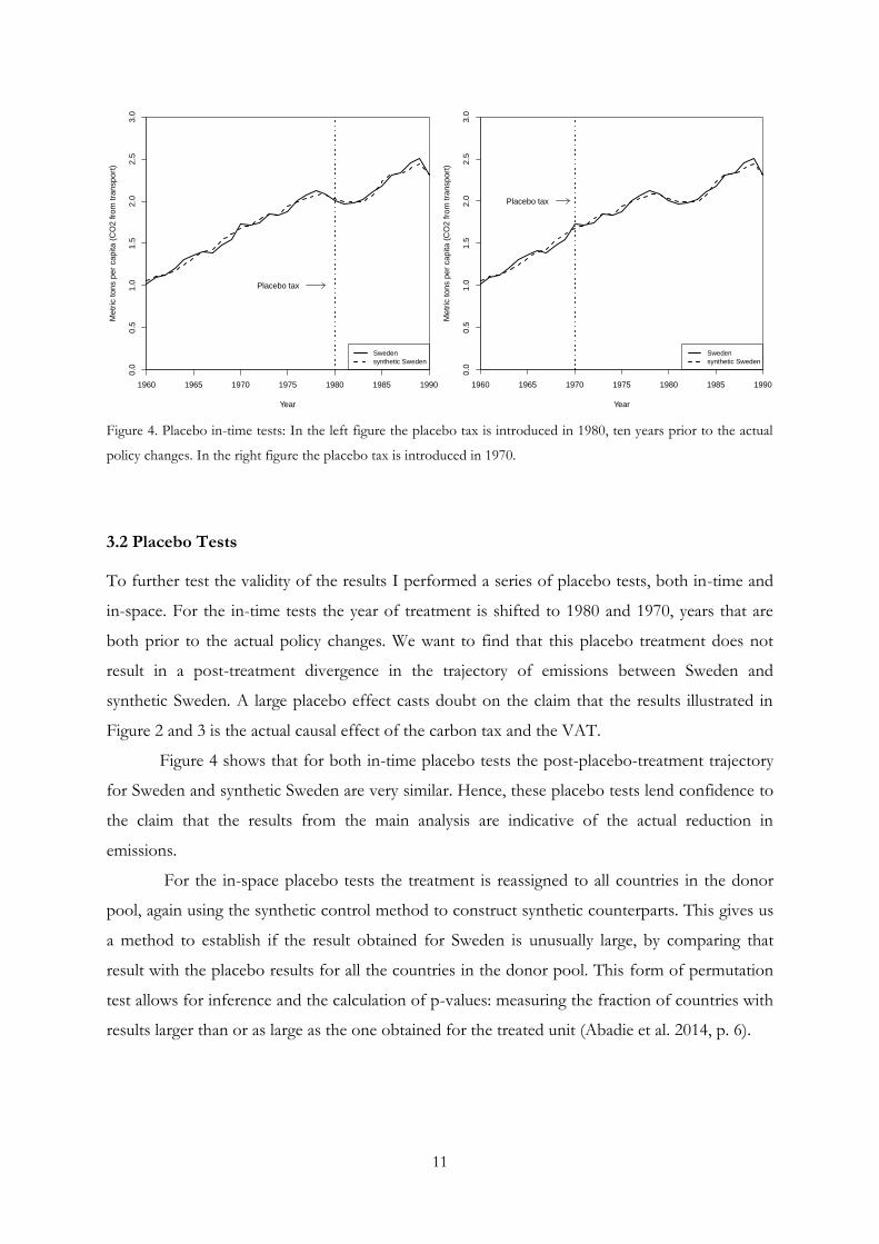
Figure 4. Placebo in-time tests: In the left figure the placebo tax is introduced in 1980, ten years prior to the actual

policy changes. In the right figure the placebo tax is introduced in 1970.

3.2 Placebo Tests

To further test the validity of the results I performed a series of placebo tests, both in-time and

in-space. For the in-time tests the year of treatment is shifted to 1980 and 1970, years that are

both prior to the actual policy changes. We want to find that this placebo treatment does not

result in a post-treatment divergence in the trajectory of emissions between Sweden and

synthetic Sweden. A large placebo effect casts doubt on the claim that the results illustrated in

Figure 2 and 3 is the actual causal effect of the carbon tax and the VAT.

Figure 4 shows that for both in-time placebo tests the post-placebo-treatment trajectory

for Sweden and synthetic Sweden are very similar. Hence, these placebo tests lend confidence to

the claim that the results from the main analysis are indicative of the actual reduction in

emissions.

For the in-space placebo tests the treatment is reassigned to all countries in the donor

pool, again using the synthetic control method to construct synthetic counterparts. This gives us

a method to establish if the result obtained for Sweden is unusually large, by comparing that

result with the placebo results for all the countries in the donor pool. This form of permutation

test allows for inference and the calculation of p-values: measuring the fraction of countries with

results larger than or as large as the one obtained for the treated unit (Abadie et al. 2014, p. 6).

1960 1965 1970 1975 1980 1985 1990

0.0

0.5

1.0

1.5

2.0

2.5

3.0

Year

Metr

ic ton

s p

er

ca

pita (

CO

2 fro

m tra

nsp

ort

)

Sweden

synthetic Sweden

Placebo tax

1960 1965 1970 1975 1980 1985 1990

0.0

0.5

1.0

1.5

2.0

2.5

3.0

Year

Metr

ic ton

s p

er

ca

pita (

CO

2 fro

m tra

nsp

ort

)

Sweden

synthetic Sweden

Placebo tax

12

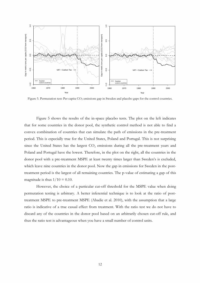
Figure 5. Permutation test: Per capita CO2 emissions gap in Sweden and placebo gaps for the control countries.

Figure 5 shows the results of the in-space placebo tests. The plot on the left indicates

that for some countries in the donor pool, the synthetic control method is not able to find a

convex combination of countries that can simulate the path of emissions in the pre-treatment

period. This is especially true for the United States, Poland and Portugal. This is not surprising

since the United States has the largest CO2 emissions during all the pre-treatment years and

Poland and Portugal have the lowest. Therefore, in the plot on the right, all the countries in the

donor pool with a pre-treatment MSPE at least twenty times larger than Sweden’s is excluded,

which leave nine countries in the donor pool. Now the gap in emissions for Sweden in the post-

treatment period is the largest of all remaining countries. The p-value of estimating a gap of this

magnitude is thus 1/10 = 0.10.

However, the choice of a particular cut-off threshold for the MSPE value when doing

permutation testing is arbitrary. A better inferential technique is to look at the ratio of post-

treatment MSPE to pre-treatment MSPE (Abadie et al. 2010), with the assumption that a large

ratio is indicative of a true casual effect from treatment. With the ratio test we do not have to

discard any of the countries in the donor pool based on an arbitrarily chosen cut-off rule, and

thus the ratio test is advantageous when you have a small number of control units.

1960 1970 1980 1990 2000

−1.0

−0

.50

.00.5

1.0

Year

Gap

in m

etr

ic ton

s p

er

cap

ita (

CO

2 f

rom

tra

nspo

rt)

Swedencontrol countries

VAT + Carbon Tax

1960 1970 1980 1990 2000

−1.0

−0

.50

.00.5

1.0

Year

Gap

in m

etr

ic ton

s p

er

cap

ita (

CO

2 f

rom

tra

nspo

rt)

Swedencontrol countries

VAT + Carbon Tax

13

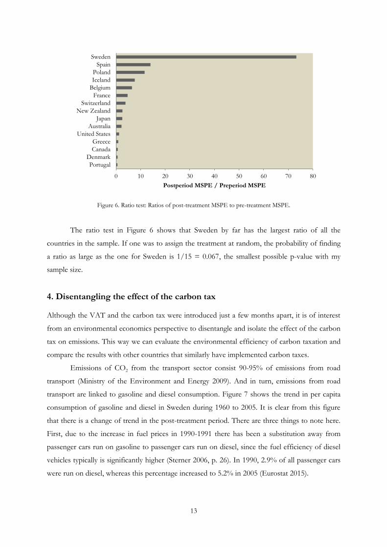
Figure 6. Ratio test: Ratios of post-treatment MSPE to pre-treatment MSPE.

The ratio test in Figure 6 shows that Sweden by far has the largest ratio of all the

countries in the sample. If one was to assign the treatment at random, the probability of finding

a ratio as large as the one for Sweden is 1/15 = 0.067, the smallest possible p-value with my

sample size.

4. Disentangling the effect of the carbon tax

Although the VAT and the carbon tax were introduced just a few months apart, it is of interest

from an environmental economics perspective to disentangle and isolate the effect of the carbon

tax on emissions. This way we can evaluate the environmental efficiency of carbon taxation and

compare the results with other countries that similarly have implemented carbon taxes.

Emissions of CO2 from the transport sector consist 90-95% of emissions from road

transport (Ministry of the Environment and Energy 2009). And in turn, emissions from road

transport are linked to gasoline and diesel consumption. Figure 7 shows the trend in per capita

consumption of gasoline and diesel in Sweden during 1960 to 2005. It is clear from this figure

that there is a change of trend in the post-treatment period. There are three things to note here.

First, due to the increase in fuel prices in 1990-1991 there has been a substitution away from

passenger cars run on gasoline to passenger cars run on diesel, since the fuel efficiency of diesel

vehicles typically is significantly higher (Sterner 2006, p. 26). In 1990, 2.9% of all passenger cars

were run on diesel, whereas this percentage increased to 5.2% in 2005 (Eurostat 2015).

0 10 20 30 40 50 60 70 80

Portugal

Denmark

Canada

Greece

United States

Australia

Japan

New Zealand

Switzerland

France

Belgium

Iceland

Poland

Spain

Sweden

Postperiod MSPE / Preperiod MSPE

14

Figure 7. Road fuel consumption per capita in Sweden during 1960-2005.

Secondly, between 1990 to 2005 the amount of lorries, semi-trailers, trailers, and tractors, which

all typically run on diesel, increased by 47%. This large increase is likely linked to amplified

shipment of goods due to globalisation, and Sweden intensifying its trade with the rest of Europe

after joining the EU in 1995. Lastly, companies which are the main users of lorries, trailers and

tractors have the VAT on fuel refunded back to them. Hence, they are only impacted by the

carbon tax and we should thus see smaller changes in their fuel consumption compared to

regular gasoline consumers, especially since the demand elasticity for diesel in Sweden is

estimated to be as low as -0.25 (Dahl 2012). Taken together, this explains why we see a large

change of trend in gasoline consumption in the post-treatment period but not a similar change in

diesel consumption.

4.1 Emission reductions due to the carbon tax

Since gasoline constitute the largest part of fuel consumption, my estimate of the emission

reductions attributable to the carbon tax uses data only for the relationship between the VAT

rate and the carbon tax rate on gasoline. Note though that this estimate serves as a lower bound

since the emission reductions attributable to changes in diesel consumption are mainly due to the

carbon tax since the VAT only affects a small percentage of the consumers of diesel.

1960 1970 1980 1990 2000

0100

200

300

400

500

600

Year

Road

secto

r fu

el co

nsum

ptio

n p

er

ca

pita (

kg o

f o

il equiv

ale

nt)

GasolineDiesel

VAT + Carbon tax

15

Figure 8. The VAT and carbon tax component of the price of gasoline in Sweden.

Since the introduction of the carbon tax there have been minor alterations in the rate of

the existing energy tax that is added to gasoline. The energy tax was increased slightly during

1992-2000 and then reduced between 2000 and 2005, while the carbon tax has been increased

over the post-treatment period. When measuring the carbon tax level in figure 8 I fixed the

energy tax at the rate applied in 1990. In 2005 the carbon tax was 910 SEK ($109) per ton of

CO2 and the calculations made in this section assume a carbon tax of 930 SEK ($111) per ton of

CO2, hence this small difference should not affect the results much.

Adding the carbon tax and the VAT together we get an average combined tax rate for

the 1990-2005 period of 1290 SEK ($155) per ton of CO2 and 1887 SEK ($226) per ton of CO2

in 2005. Compared to the actual carbon tax rate in 2014, the average combined tax rate is 17%

higher and the 2005 combined rate is 72% higher.

In 2005 the carbon tax comprised close to 50% of the combined rate of the carbon tax

and the VAT. Making a rough assumption that this percentage translates into reductions in CO2

emissions associated to the carbon tax gives a reduction in 2005 of 6.2%, or -0.17 metric tons of

CO2 per capita. Over the entire post-treatment period the carbon tax has comprised 40% of the

combined tax rate and led to emission reductions of 4.9%, equivalent to -0.13 metric tons of

CO2 per capita in an average year. Aggregating over the total population gives an emission

reduction, attributable to the carbon tax, of 1.6 million metric tons of CO2 in 2005 and an annual

average for the 1990-2005 period of 1.1 million metric tons of CO2.

0.00

0.50

1.00

1.50

2.00

2.50

1990 1992 1994 1996 1998 2000 2002 2004

SEK/litre

Year

VAT

Carbon Tax

16

4.2 Estimates from previous literature

My estimated emission reductions can be compared to previous estimates from analyses of the

Swedish carbon tax. However, most analyses are ex-ante modelling studies and very few are ex-

post empirical studies, and even fewer look at the transport sector in isolation.

In Bohlin (1998) the author concludes that during 1990-1995 the carbon tax had no

impact on emissions from the transport sector. I instead find an average emission reduction of

2.6% during 1990-1995 attributed to the carbon tax with a reduction in 1995 alone of 5%.

Sweden’s fifth national report on climate change (Ministry of the Environment and

Energy 2009) estimates that the reduction of CO2 emissions from the transport sector in 2005 is

1.7 million metric tons compared to if Sweden had kept taxes at the 1990 level. The emissions

reduction is modelled by estimating changes in fuel consumption, using price elasticities of

demand for fuel. However, the report does not clearly specify if the effect of the introduction of

VAT in 1990 is included or not in their estimates, making it harder to compare their results with

mine. If VAT is included, then their estimate is markedly lower compared to my estimate of

emissions reduction in 2005 of 3.2 million metric tons of CO2. If the VAT is not included, which

is more likely, their estimate of a reduction of 1.7 million metric tons is close to my estimate of

1.6 million metric tons (from the carbon tax alone), but their methodology is then flawed since

they do not take into account the long-term effect on emissions from the introduction of the

VAT just a few months prior to the start date of their calculations.

5. Conclusion

In the environmental economics literature on climate change there is much emphasis on carbon

taxation as an environmentally and economically efficient way to reduce greenhouse gases.

However, there are very few real world examples of countries implementing carbon taxes and

even fewer ex-post studies that capture the causal effect on emissions from these taxes.

In this paper I have estimated the reduction in CO2 emissions from the transport sector

in Sweden following the introduction of a carbon tax and VAT in the years 1990-1991. With the

use of the synthetic control method I estimate the causal effect to be a reduction in emissions of

10.9% during the post-treatment period of 1990-2005, equivalent to 2.5 million metric tons of

CO2 in the annual total. Looking at the effect of the carbon tax in isolation I estimate a post-

treatment reduction of 4.9%, equivalent to 1.1 million metric tons of CO2 in an average year.

Synthetic Sweden is able to very accurately reproduce the values for Sweden on a number

of key predictors of CO2 emissions from the transport sector, and to closely track emissions

during the thirty years prior to treatment. The results are furthermore robust to a series of

17

placebo tests, both in-time and in-space. Reassigning the treatment at random in the sample

shows that the probability of obtaining a post-treatment result as large as that for Sweden is just

0.067. Combined, the results of the analysis and the robustness tests lend weight to the claim

that the estimated emission reductions capture the causal effect of the policy changes in Sweden.

18

Appendix: Data Sources

CO2 emissions from transport. Measured in metric tons per capita. Source: the World

Bank WDI Database. Available at: data.worldbank.org/indicator.

GDP per capita (PPP, 2005 USD). Expenditure-side real GDP at chained PPPs, divided

by population. Source: Feenstra, Robert C., Robert Inklaar and Marcel P. Timmer (2013),

“The Next Generation of the Penn World Table”. Available at: www.ggdc.net/pwt.

Motor Vehicles (per 1000 people). Source: Dargay, Joyce, Dermot Gately and Martin

Sommer (2007), “Vehicle Ownership and Income Growth, Worldwide: 1960-2030”.

Gasoline consumption per capita. Measured in kg of oil equivalent. Source: the World

Bank WDI Database. Available at: data.worldbank.org/indicator.

Urban Population. Measured in percentage of total. Source: the World Bank WDI

Database. Available at: data.worldbank.org/indicator.

19

References

ABADIE, A., A. DIAMOND, and J. HAINMUELLER (2010): "Synthetic Control Methods for Comparative

Case Studies: Estimating the Effect of California's Tobacco Control Program," Journal of the

American Statistical Association, 105, 493-505.

ABADIE, A., A. DIAMOND, and J. HAINMUELLER (2011): "Synth: An R Package for Synthetic Control

Methods in Comparative Case Studies," Journal of Statistical Software, 42, 1-17.

ABADIE, A., A. DIAMOND, and J. HAINMUELLER (2014): "Comparative Politics and the Synthetic

Control Method," American Journal of Political Science.

ABADIE, A., and J. GARDEAZABAL (2003): "The Economic Costs of Conflict: A Case Study of the

Basque Country," American Economic Review, 93, 113-132.

ANDERSEN, M. S., N. DENGSØE, and A. B. PEDERSEN (2001): An Evaluation of the Impact of Green Taxes in

the Nordic Countries. Nordic Council of Ministers.

BOHLIN, F. (1998): "The Swedish Carbon Dioxide Tax: Effects on Biofuel Use and Carbon Dioxide

Emissions," Biomass and bioenergy, 15, 283-291.

DAHL, C. A. (2012): "Measuring Global Gasoline and Diesel Price and Income Elasticities," Energy Policy,

41, 2-13.

DARGAY, J., D. GATELY, and M. SOMMER (2007): "Vehicle Ownership and Income Growth, Worldwide:

1960-2030," The Energy Journal, 143-170.

EUROPEAN FEDERATION FOR TRANSPORT AND ENVIRONMENT (2011): Fuelling Oil Demand: What

happened to fuel taxation in Europe? Brussels, Belgium.

GATELY, C. K., L. R. HUTYRA, and I. S. WING (2015): "Cities, Traffic, and Co2: A Multidecadal

Assessment of Trends, Drivers, and Scaling Relationships," Proceedings of the National Academy of

Sciences, 112, 4999-5004.

HOLLAND, P. W. (1986): "Statistics and Causal Inference," Journal of the American Statistical Association, 81,

945-960.

LIN, B., and X. LI (2011): "The Effect of Carbon Tax on Per Capita Co 2 Emissions," Energy Policy, 39,

5137-5146.

MINISTRY OF THE ENVIRONMENT AND ENERGY (2009): “Sveriges femte nationalrapport om

klimatförändringar,” Ds 2009:63. Available at: http://www.riksdagen.se/sv/Dokument-

Lagar/Utredningar/Departementsserien/Sveriges-femte-nationalrapport_GXB463/?html=true.

NEUMAYER, E. (2004): “National carbon dioxode emissions: geography matter,” Area, 36.1, 33-40.

STERNER, T. (2006): Survey of Transport Fuel Demand Elasticities. Swedish Environmental Protection Agency.

Report 5586, September 2006. Stockholm, Sweden.