Fast Kernel Learning for Multidimensional PatternExtrapolation

Andrew Gordon Wilson∗Carnegie Mellon Universityandrewgw@cs.cmu.edu

Elad Gilboa∗Washington University St. Louisgilboae@ese.wustl.edu

Arye NehoraiWashington University St. Louisnehorai@ese.wustl.edu

John P. CunninghamColumbia University

jpc2181@columbia.edu

Abstract

The ability to automatically discover patterns and perform extrapolation is an es-sential quality of intelligent systems. Kernel methods, such as Gaussian processes,have great potential for pattern extrapolation, since the kernel flexibly and inter-pretably controls the generalisation properties of these methods. However, auto-matically extrapolating large scale multidimensional patterns is in general diffi-cult, and developing Gaussian process models for this purpose involves severalchallenges. A vast majority of kernels, and kernel learning methods, currentlyonly succeed in smoothing and interpolation. This difficulty is compounded bythe fact that Gaussian processes are typically only tractable for small datasets, andscaling an expressive kernel learning approach poses different challenges thanscaling a standard Gaussian process model. One faces additional computationalconstraints, and the need to retain significant model structure for expressing therich information available in a large dataset. In this paper, we propose a Gaussianprocess approach for large scale multidimensional pattern extrapolation. We re-cover sophisticated out of class kernels, perform texture extrapolation, inpainting,and video extrapolation, and long range forecasting of land surface temperatures,all on large multidimensional datasets, including a problem with 383,400 trainingpoints. The proposed method significantly outperforms alternative scalable andflexible Gaussian process methods, in speed and accuracy. Moreover, we showthat a distinct combination of expressive kernels, a fully non-parametric represen-tation, and scalable inference which exploits existing model structure, are criticalfor large scale multidimensional pattern extrapolation.

1 Introduction

Our ability to effortlessly extrapolate patterns is a hallmark of intelligent systems: even with largemissing regions in our field of view, we can see patterns and textures, and we can visualise in ourmind how they generalise across space. Indeed machine learning methods aim to automaticallylearn and generalise representations to new situations. Kernel methods, such as Gaussian processes(GPs), are popular machine learning approaches for non-linear regression and classification [1, 2, 3].Flexibility is achieved through a kernel function, which implicitly represents an inner product ofarbitrarily many basis functions. The kernel interpretably controls the smoothness and generalisationproperties of a GP. A well chosen kernel leads to impressive empirical performances [2].

However, it is extremely difficult to perform large scale multidimensional pattern extrapolation withkernel methods. In this context, the ability to learn a representation of the data entirely depends

∗Authors contributed equally.

1

on learning a kernel, which is a priori unknown. Moreover, kernel learning methods [4] are nottypically intended for automatic pattern extrapolation; these methods often involve hand craftingcombinations of Gaussian kernels (for smoothing and interpolation), for specific applications suchas modelling low dimensional structure in high dimensional data. Without human intervention,the vast majority of existing GP models are unable to perform pattern discovery and extrapolation.While recent approaches such as [5] enable extrapolation on small one dimensional datasets, it isdifficult to generalise these approaches for larger multidimensional situations. These difficultiesarise because Gaussian processes are computationally intractable on large scale data, and whilescalable approximate GP methods have been developed [6, 7, 8, 9, 10, 11, 12, 13], it is uncertainhow to best scale expressive kernel learning approaches. Furthermore, the need for flexible kernellearning on large datasets is especially great, since such datasets often provide more information tolearn an appropriate statistical representation.

In this paper, we introduce GPatt, a flexible, non-parametric, and computationally tractable ap-proach to kernel learning for multidimensional pattern extrapolation, with particular applicabilityto data with grid structure, such as images, video, and spatial-temporal statistics. Specifically, thecontributions of this paper include:

• We extend fast and exact Kronecker-based GP inference (e.g., [14]) to account for non-grid data.Our experiments include data where more than 70% of the training data are not on a grid. Byadapting expressive spectral mixture kernels to the setting of multidimensional inputs and Kro-necker structure, we achieve exact inference and learning costs of O(PN P+1

P ) computations andO(PN 2

P ) storage, for N datapoints and P input dimensions, compared to the standard O(N3)computations and O(N2) storage associated with a Cholesky decomposition.

• We show that this combination of i) spectral mixture kernels (adapted for Kronecker structure);ii) scalable inference based on Kronecker methods (adapted for incomplete grids); and, iii) trulynon-parametric representations, when used in combination (to form GPatt) distinctly enable large-scale multidimensional pattern extrapolation with GPs. We demonstrate this through a compar-ison with various expressive models and inference techniques: i) spectral mixture kernels witharguably the most popular scalable GP inference method (FITC) [10]; ii) a fast and efficient re-cent spectral based kernel learning method (SSGP) [6]; and, iii) the most popular GP kernels withKronecker based inference.

• The information capacity of non-parametric methods grows with the size of the data. A trulynon-parametric GP must have a kernel that is derived from an infinite basis function expansion.We find that a truly non-parametric representation is necessary for pattern extrapolation on largedatasets, and provide insights into this surprising result.

• GPatt is highly scalable and accurate. This is the first time, as far as we are aware, that highlyexpressive non-parametric kernels with in some cases hundreds of hyperparameters, on datasetsexceeding N = 105 training instances, can be learned from the marginal likelihood of a GP, inonly minutes. Such experiments drive home the point that one can, to some extent, solve kernelselection, and automatically extract useful features from the data, on large datasets, using a specialcombination of expressive kernels and scalable inference.

• We show that the proposed methodology is rather distinct, as a GP model, in its ability to approachtexture extrapolation and inpainting. It was not previously known how to make GPs work for thesefundamental applications.

• Moreover, unlike typical inpainting approaches, such as patch-based methods (which work byrecursively copying pixels or patches into a gap in an image, preserving neighbourhood similar-ities), GPatt is not restricted to spatial inpainting. This is demonstrated on a video extrapolationexample, for which standard inpainting methods would be inapplicable [15]. Similarly, we applyGPatt to perform large-scale long range forecasting of land surface temperatures, through learninga sophisticated correlation structure across space and time. This learned correlation structure alsoprovides insights into the underlying statistical properties of these data.

• We demonstrate that GPatt can precisely recover sophisticated out-of-class kernels automatically.

2 Spectral Mixture Product Kernels for Pattern Discovery

The spectral mixture kernel has recently been introduced [5] to offer a flexible kernel that can learnany stationary kernel. By appealing to Bochner’s theorem [16] and building a scale mixture of A

2

Gaussian pairs in the spectral domain, [5] produced the spectral mixture kernel:

kSM(τ) =

A∑a=1

w2aexp{−2π2τ2σ2

a} cos(2πτµa), (1)

which they applied to a small number of one-dimensional input data. For tractability with multidi-mensional inputs and large data, we propose a spectral mixture product (SMP) kernel:

kSMP(τ |θ) =P∏p=1

kSM(τp|θp) , (2)

where τp is the pth component of τ = x− x′ ∈ RP , θp are the hyperparameters {µa, σ2a, w

2a}Aa=1 of

the pth spectral mixture kernel in the product of Eq. (2), and θ = {θp}Pp=1 are the hyperparametersof the SMP kernel. The SMP kernel of Eq. (2) has Kronecker structure which we exploit for scalableand exact inference in section 2.1. With enough componentsA, the SMP kernel of Eq. (2) can modelany stationary product kernel to arbitrary precision, and is flexible even with a small number ofcomponents, since scale-location Gaussian mixture models can approximate many spectral densities.We use SMP-A as shorthand for an SMP kernel with A components in each dimension (for a totalof 3PA kernel hyperparameters and 1 noise hyperparameter).

Critically, a GP with an SMP kernel is not a finite basis function method, but instead corresponds toa finite (A component) mixture of infinite basis function expansions. Therefore such a GP is a trulynonparametric method. This difference between a truly nonparametric representation – namely amixture of infinite bases – and a parametric kernel method, a finite basis expansion correspondingto a degenerate GP, is critical both conceptually and practically, as our results will show.

2.1 Fast Exact Inference with Spectral Mixture Product Kernels

Gaussian process inference and learning requires evaluating (K+σ2I)−1y and log |K+σ2I|, for anN ×N covariance matrix K, a vector of N datapoints y, and noise variance σ2, as described in thesupplementary material. For this purpose, it is standard practice to take the Cholesky decompositionof (K + σ2I) which requires O(N3) computations and O(N2) storage, for a dataset of size N .However, many real world applications are engineered for grid structure, including spatial statistics,sensor arrays, image analysis, and time sampling. [14] has shown that the Kronecker structurein product kernels can be exploited for exact inference and hyperparameter learning in O(PN 2

P )

storage and O(PN P+1P ) operations, so long as the inputs x ∈ X are on a multidimensional grid,

meaning X = X1 × · · · × XP ⊂ RP . Details are in the supplement.

Here we relax this grid assumption. Assuming we have a dataset of M observations which arenot necessarily on a grid, we propose to form a complete grid using W imaginary observations,yW ∼ N (fW , ε

−1IW ), ε → 0. The total observation vector y = [yM ,yW ]> has N = M +Wentries: y = N (f , DN ), where the noise covariance matrix DN = diag(DM , ε

−1IW ), DM =σ2IM . The imaginary observations yW have no corrupting effect on inference: the moments ofthe resulting predictive distribution are exactly the same as for the standard predictive distribution,namely limε→0(KN +DN )−1y = (KM +DM )−1yM (proof in the supplement).

We use preconditioned conjugate gradients (PCG) [17] to compute (KN +DN )−1

y. We use thepreconditioning matrix C = D

−1/2N to solve C> (KN +DN )Cz = C>y. The preconditioning

matrix C speeds up convergence by ignoring the imaginary observations yW . Exploiting the fastmultiplication of Kronecker matrices, PCG takes O(JPN P+1

P ) total operations (where the numberof iterations J � N ) to compute (KN +DN )

−1y to convergence within machine precision.

For learning (hyperparameter training) we must evaluate the marginal likelihood (supplement). Wecannot efficiently decompose KM +DM to compute the log |KM +DM | complexity penalty in themarginal likelihood, because KM is not a Kronecker matrix and DM is not a scaled identity (as isthe usual case for Kronecker decompositions). We approximate the complexity penalty as

log |KM +DM | =M∑i=1

log(λMi + σ2) ≈M∑i=1

log(λMi + σ2) , (3)

3

where σ is the noise standard deviation of the data. We approximate the eigenvalues λMi of KM

using the eigenvalues ofKN such that λMi = MN λ

Ni for i = 1, . . . ,M , which is particularly effective

for large M (e.g. M > 1000) [7]. Notably, only the log determinant (complexity penalty) term inthe marginal likelihood undergoes a small approximation, and inference remains exact.

All remaining terms in the marginal likelihood can be computed exactlyly and efficiently using PCG.The total runtime cost of hyperparameter learning and exact inference with an incomplete grid is thusO(PN P+1

P ). In image problems, for example, P = 2, and so the runtime complexity reduces toO(N1.5). Although the proposed inference can handle non-grid data, this inference is most suitedto inputs where there is some grid structure – images, video, spatial statistics, etc. If there is nosuch grid structure (e.g., none of the training data fall onto a grid), then the computational expensenecessary to augment the data with imaginary grid observations can be prohibitive.

3 Experiments

In our experiments we combine the SMP kernel of Eq. (2) with the fast exact inference and learningprocedures of section 2.1, in a GP method we henceforth call GPatt1,2.

We contrast GPatt with many alternative Gaussian process kernel methods. We are particularlyinterested in kernel methods, since they are considered to be general purpose regression methods, butconventionally have difficulty with large scale multidimensional pattern extrapolation. Specifically,we compare to the recent sparse spectrum Gaussian process regression (SSGP) [6] method, whichprovides fast and flexible kernel learning. SSGP models the kernel spectrum (spectral density)as a sum of point masses, such that SSGP is a finite basis function (parametric) model, with asmany basis functions as there are spectral point masses. SSGP is similar to the recent models ofLe et al. [8] and Rahimi and Recht [9], except it learns the locations of the point masses throughmarginal likelihood optimization. We use the SSGP implementation provided by the authors athttp://www.tsc.uc3m.es/˜miguel/downloads.php.

To further test the importance of the fast inference (section 2.1) used in GPatt, we compare to aGP which uses the SMP kernel of section 2 but with the popular fast FITC [10, 18] inference,implemented in GPML (http://www.gaussianprocess.org/gpml). We also compare toGPs with the popular squared exponential (SE), rational quadratic (RQ) and Matern (MA) (with 3degrees of freedom) kernels, catalogued in Rasmussen and Williams [1], respectively for smooth,multi-scale, and finitely differentiable functions. Since GPs with these kernels cannot scale to thelarge datasets we consider, we combine these kernels with the same fast inference techniques thatwe use with GPatt, to enable a comparison.3 Moreover, we stress test each of these methods interms of speed and accuracy, as a function of available data and extrapolation range, and number ofcomponents. All of our experiments contain a large percentage of missing (non-grid) data, and wetest accuracy and efficiency as a function of the percentage of missing data.

In all experiments we assume Gaussian noise, to express the marginal likelihood of the data p(y|θ)solely as a function of kernel hyperparameters θ. To learn θ we optimize the marginal likelihoodusing BFGS. We use a simple initialisation scheme: any frequencies {µa} are drawn from a uniformdistribution from 0 to the Nyquist frequency (1/2 the sampling rate), length-scales {1/σa} from atruncated Gaussian distribution, with mean proportional to the range of the data, and weights {wa}are initialised as the empirical standard deviation of the data divided by the number of componentsused in the model. In general, we find GPatt is robust to initialisation, particularly for N > 104

datapoints. We show a representative initialisation in the experiments.

This range of tests allows us to separately understand the effects of the SMP kernel, a non-parametricrepresentation, and the proposed inference methods of section 2.1; we will show that all are requiredfor good extrapolation performance.

1We write GPatt-A when GPatt uses an SMP-A kernel.2Experiments were run on a 64bit PC, with 8GB RAM and a 2.8 GHz Intel i7 processor.3We also considered the model of [19], but this model is intractable for the datasets we considered and is

not structured for the fast inference of section 2.1.

4

3.1 Extrapolating Metal Tread Plate and Pores Patterns

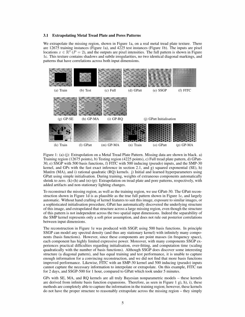
We extrapolate the missing region, shown in Figure 1a, on a real metal tread plate texture. Thereare 12675 training instances (Figure 1a), and 4225 test instances (Figure 1b). The inputs are pixellocations x ∈ R2 (P = 2), and the outputs are pixel intensities. The full pattern is shown in Figure1c. This texture contains shadows and subtle irregularities, no two identical diagonal markings, andpatterns that have correlations across both input dimensions.

(a) Train

(b) Test (c) Full (d) GPatt (e) SSGP (f) FITC

(g) GP-SE (h) GP-MA (i) GP-RQ (j) GPatt Initialisation

(k) Train (l) GPatt (m) GP-MA (n) Train (o) GPatt (p) GP-MA

Figure 1: (a)-(j): Extrapolation on a Metal Tread Plate Pattern. Missing data are shown in black. a)Training region (12675 points), b) Testing region (4225 points), c) Full tread plate pattern, d) GPatt-30, e) SSGP with 500 basis functions, f) FITC with 500 inducing (pseudo) inputs, and the SMP-30kernel, and GPs with the fast exact inference in section 2.1, and g) squared exponential (SE), h)Matern (MA), and i) rational quadratic (RQ) kernels. j) Initial and learned hyperparameters usingGPatt using simple initialisation. During training, weights of extraneous components automaticallyshrink to zero. (k)-(h) and (n)-(p): Extrapolation on tread plate and pore patterns, respectively, withadded artifacts and non-stationary lighting changes.

To reconstruct the missing region, as well as the training region, we use GPatt-30. The GPatt recon-struction shown in Figure 1d is as plausible as the true full pattern shown in Figure 1c, and largelyautomatic. Without hand crafting of kernel features to suit this image, exposure to similar images, ora sophisticated initialisation procedure, GPatt has automatically discovered the underlying structureof this image, and extrapolated that structure across a large missing region, even though the structureof this pattern is not independent across the two spatial input dimensions. Indeed the separability ofthe SMP kernel represents only a soft prior assumption, and does not rule out posterior correlationsbetween input dimensions.

The reconstruction in Figure 1e was produced with SSGP, using 500 basis functions. In principleSSGP can model any spectral density (and thus any stationary kernel) with infinitely many compo-nents (basis functions). However, since these components are point masses (in frequency space),each component has highly limited expressive power. Moreover, with many components SSGP ex-periences practical difficulties regarding initialisation, over-fitting, and computation time (scalingquadratically with the number of basis functions). Although SSGP does discover some interestingstructure (a diagonal pattern), and has equal training and test performance, it is unable to captureenough information for a convincing reconstruction, and we did not find that more basis functionsimproved performance. Likewise, FITC with an SMP-30 kernel and 500 inducing (pseudo) inputscannot capture the necessary information to interpolate or extrapolate. On this example, FITC ranfor 2 days, and SSGP-500 for 1 hour, compared to GPatt which took under 5 minutes.

GPs with SE, MA, and RQ kernels are all truly Bayesian nonparametric models – these kernelsare derived from infinite basis function expansions. Therefore, as seen in Figure 1 g), h), i), thesemethods are completely able to capture the information in the training region; however, these kernelsdo not have the proper structure to reasonably extrapolate across the missing region – they simply

5

(a) Runtime Stress Test (b) Accuracy Stress Test

0 500

0.5

1

τ

k1

0 500

0.5

1

τ

k2

0 500

0.5

1

τ

k3

TrueRecovered

(c) Recovering Sophisticated Kernels

Figure 2: Stress Tests. a) Runtime Stress Test. We show the runtimes in seconds, as a functionof training instances, for evaluating the log marginal likelihood, and any relevant derivatives, for astandard GP with SE kernel (as implemented in GPML), FITC with 500 inducing (pseudo) inputsand SMP-25 and SMP-5 kernels, SSGP with 90 and 500 basis functions, and GPatt-100, GPatt-25,and GPatt-5. Runtimes are for a 64bit PC, with 8GB RAM and a 2.8 GHz Intel i7 processor, on thecone pattern (P = 2), shown in the supplement. The ratio of training inputs to the sum of imaginaryand training inputs for GPatt is 0.4 and 0.6 for the smallest two training sizes, and 0.7 for all othertraining sets. b) Accuracy Stress Test. MSLL as a function of holesize on the metal pattern ofFigure 1. The values on the horizontal axis represent the fraction of missing (testing) data fromthe full pattern (for comparison Fig 1a has 25% missing data). We compare GPatt-30 and GPatt-15with GPs with SE, MA, and RQ kernels (and the inference of section 2.1), and SSGP with 100 basisfunctions. The MSLL for GPatt-15 at a holesize of 0.01 is −1.5886. c) Recovering SophisticatedKernels. A product of three kernels (shown in green) was used to generate a movie of 112,500training points. From this data, GPatt-20 reconstructs these component kernels (the learned SMP-20kernel is shown in blue). All kernels are a function of τ = x− x′. has been scaled by k(0).

act as smoothing filters. We note that this comparison is only possible because these GPs are usingthe fast exact inference techniques in section 2.1.

Overall, these results indicate that both expressive nonparametric kernels, such as the SMP kernel,and the specific fast inference in section 2.1, are needed to extrapolate patterns in these images.

We note that the SMP-30 kernel used with GPatt has more components than needed for this problem.However, as shown in Fig. 1j, if the model is overspecified, the complexity penalty in the marginallikelihood shrinks the weights ({wa} in Eq. (1)) of extraneous components, as a proxy for modelselection – an effect similar to automatic relevance determination [20]. Components which donot significantly contribute to model fit will therefore be automatically pruned, as shrinking theweights decreases the eigenvalues of K and thus minimizes the complexity penalty (a sum of logeigenvalues). This simple GPatt initialisation procedure was used for the results in all experimentsand is especially effective for N > 104 points.

In Figure 1 (k)-(h) and (n)-(p) we use GPatt to extrapolate on treadplate and pore patterns with addedartifacts and lighting changes. GPatt still provides a convincing extrapolation – able to uncover bothlocal and global structure. Alternative GPs with the inference of section 2.1 can interpolate smallartifacts quite accurately, but have trouble with larger missing regions.

3.2 Stress Tests and Recovering Complex 3D Kernels from Video

We stress test GPatt and alternative methods in terms of speed and accuracy, with varying data-sizes, extrapolation ranges, basis functions, inducing (pseudo) inputs, and components. We assessaccuracy using standardised mean square error (SMSE) and mean standardized log loss (MSLL) (ascaled negative log likelihood), as defined in Rasmussen and Williams [1] on page 23. Using theempirical mean and variance to fit the data would give an SMSE and MSLL of 1 and 0 respectively.Smaller SMSE and more negative MSLL values correspond to better fits of the data.

The runtime stress test in Figure 2a shows that the number of components used in GPatt does notsignificantly affect runtime, and that GPatt is much faster than FITC (using 500 inducing inputs) andSSGP (using 90 or 500 basis functions), even with 100 components (601 kernel hyperparameters).The slope of each curve roughly indicates the asymptotic scaling of each method. In this experiment,the standard GP (with SE kernel) has a slope of 2.9, which is close to the cubic scaling we expect. All

6

Table 1: We compare the test performance of GPatt-30 with SSGP (using 100 basis functions), andGPs using squared exponential (SE), Matern (MA), and rational quadratic (RQ) kernels, combinedwith the inference of section 3.2, on patterns with a train test split as in the metal treadplate patternof Figure 1. We show the results as SMSE (MSLL).

Rubber mat Tread plate Pores Wood Chain mailtrain, test 12675, 4225 12675, 4225 12675, 4225 14259, 4941 14101, 4779

GPatt 0.31 (−0.57) 0.45 (−0.38) 0.0038 (−2.8) 0.015 (−1.4) 0.79 (−0.052)SSGP 0.65 (−0.21) 1.06 (0.018) 1.04 (−0.024) 0.19 (−0.80) 1.1 (0.036)SE 0.97 (0.14) 0.90 (−0.10) 0.89 (−0.21) 0.64 (1.6) 1.1 (1.6)MA 0.86 (−0.069) 0.88 (−0.10) 0.88 (−0.24) 0.43 (1.6) 0.99 (0.26)RQ 0.89 (0.039) 0.90 (−0.10) 0.88 (−0.048) 0.077 (0.77) 0.97 (−0.0025)

other curves have a slope of 1± 0.1, indicating linear scaling with the number of training instances.However, FITC and SSGP are used here with a fixed number of inducing inputs and basis functions.More inducing inputs and basis functions should be used when there are more training instances –and these methods scale quadratically with inducing inputs and basis functions for a fixed numberof training instances. GPatt, on the other hand, can scale linearly in runtime as a function of trainingsize, without any deterioration in performance. Furthermore, the fixed 2-3 orders of magnitudeGPatt outperforms alternatives are as practically important as asymptotic scaling.

The accuracy stress test in Figure 2b shows extrapolation (MSLL) performance on the metal treadplate pattern of Figure 1c with varying holesizes, running from 0% to 60% missing data for testing(for comparison the hole in Fig 1a has 25% missing data). GPs with SE, RQ, and MA kernels (andthe fast inference of section 2.1) all steadily increase in error as a function of holesize. Conversely,SSGP does not increase in error as a function of holesize – with finite basis functions SSGP cannotextract as much information from larger datasets as the alternatives. GPatt performs well relative tothe other methods, even with a small number of components. GPatt is particularly able to exploit theextra information in additional training instances: only when the holesize is so large that over 60%of the data are missing does GPatt’s performance degrade to the same level as alternative methods.

In Table 1 we compare the test performance of GPatt with SSGP, and GPs using SE, MA, and RQkernels, for extrapolating five different patterns, with the same train test split as for the tread platepattern in Figure 1. All patterns are shown in the supplement. GPatt consistently has the lowestSMSE and MSLL. Note that many of these datasets are sophisticated patterns, containing intricatedetails which are not strictly periodic, such as lighting irregularities, metal impurities, etc. IndeedSSGP has a periodic kernel (unlike the SMP kernel which is not strictly periodic), and is capable ofmodelling multiple periodic components, but does not perform as well as GPatt on these examples.

We also consider a particularly large example, where we use GPatt-10 to perform learning and exactinference on the Pores pattern, with 383,400 training points, to extrapolate a large missing regionwith 96,600 test points. The SMSE is 0.077, and the total runtime was 2800 seconds. Images of thesuccessful extrapolation are shown in the supplement.

We end this section by showing that GPatt can accurately recover a wide range of kernels, even usinga small number of components. To test GPatt’s ability to recover ground truth kernels, we simulatea 50 × 50 × 50 movie of data (e.g. two spatial input dimensions, one temporal) using a GP withkernel k = k1k2k3 (each component kernel in this product operates on a different input dimension),where k1 = kSE +kSE×kPER, k2 = kMA×kPER +kMA×kPER, and k3 = (kRQ +kPER)×kPER +kSE.(kPER(τ) = exp[−2 sin2(π τ ω)/`2], τ = x − x′). We use 5 consecutive 50 × 50 slices for testing,leaving a large numberN = 112500 of training points, providing much information to learn the truegenerating kernels. Moreover, GPatt-20 reconstructs these complex out of class kernels in under 10minutes, as shown in Fig 2c. In the supplement, we show true and predicted frames from the movie.

3.3 Wallpaper and Scene Reconstruction and Long Range Temperature Forecasting

Although GPatt is a general purpose regression method, it can also be used for inpainting: imagerestoration, object removal, etc. We first consider a wallpaper image stained by a black apple mark,shown in Figure 3. To remove the stain, we apply a mask and then separate the image into itsthree channels (red, green, and blue), resulting in 15047 pixels in each channel for training. In each

7

(a) Inpainting

0 50 1000

0.5

1

Time [mon]0 50

0.2

0.4

0.6

0.8

Y [Km]0 50

0

0.5

1

Cor

rela

tions

X [Km]

(b) Learned GPatt Kernel for Temperatures

0 5

0.20.40.60.8

Time [mon]0 50

0.20.40.60.8

Y [Km]0 20 40

0.20.40.60.8

Cor

rela

tions

X [Km]

(c) Learned GP-SE Kernel for Temperatures

Figure 3: a) Image inpainting with GPatt. From left to right: A mask is applied to the original image,GPatt extrapolates the mask region in each of the three (red, blue, green) image channels, and theresults are joined to produce the restored image. Top row: Removing a stain (train: 15047 × 3).Bottom row: Removing a rooftop to restore a natural scene (train: 32269×3). We do not extrapolatethe coast. (b)-(c): Kernels learned for land surface temperatures using GPatt and GP-SE.

channel we ran GPatt using SMP-30. We then combined the results from each channel to restore theimage without any stain, which is impressive given the subtleties in the pattern and lighting.

In our next example, we wish to reconstruct a natural scene obscured by a prominent rooftop, shownin the second row of Figure 3a). By applying a mask, and following the same procedure as forthe stain, this time with 32269 pixels in each channel for training, GPatt reconstructs the scenewithout the rooftop. This reconstruction captures subtle details, such as waves, with only a singletraining image. In fact this example has been used with inpainting algorithms which were givenaccess to a repository of thousands of similar images [21]. The results emphasized that conventionalinpainting algorithms and GPatt have profoundly different objectives, which are sometimes even atcross purposes: inpainting attempts to make the image look good to a human (e.g., the example in[21] placed boats in the water), while GPatt is a general purpose regression algorithm, which simplyaims to make accurate predictions at test input locations, from training data alone. For example,GPatt can naturally learn temporal correlations to make predictions in the video example of section3.2, for which standard patch based inpainting methods would be inapplicable [15].

Similarly, we use GPatt to perform long range forecasting of land surface temperatures. After train-ing on 108 months (9 years) of temperature data across North America (299,268 training points; a71 × 66 × 108 grid, with missing data for water), we forecast 12 months (1 year) ahead (33,252testing points). The runtime was under 30 minutes. The learned kernels using GPatt and GP-SE areshown in Figure 3 b) and c). The learned kernels for GPatt are highly non-standard – both quasiperiodic and heavy tailed. These learned correlation patterns provide insights into features (such asseasonal influences) which affect how temperatures are varying in space and time. Indeed learningthe kernel allows us to discover fundamental properties of the data. The temperature forecasts usingGPatt and GP-SE, superimposed on maps of North America, are shown in the supplement.

4 Discussion

Large scale multidimensional pattern extrapolation problems are of fundamental importance in ma-chine learning, where we wish to develop scalable models which can make impressive generalisa-

8

tions. However, there are many obstacles towards applying popular kernel methods, such as Gaus-sian processes, to these fundamental problems. We have shown that a combination of expressivekernels, truly Bayesian nonparametric representations, and inference which exploits model struc-ture, can distinctly enable a kernel approach to these problems. Moreover, there is much promisein further exploring Bayesian nonparametric kernel methods for large scale pattern extrapolation.Such methods can be extremely expressive, and expressive methods are most needed for large scaleproblems, which provide relatively more information for automatically learning a rich statisticalrepresentation of the data.

References[1] C.E. Rasmussen and C.K.I. Williams. Gaussian processes for Machine Learning. The MIT

Press, 2006.[2] C.E. Rasmussen. Evaluation of Gaussian Processes and Other Methods for Non-linear Re-

gression. PhD thesis, University of Toronto, 1996.[3] Anthony O’Hagan. Curve fitting and optimal design for prediction. Journal of the Royal

Statistical Society, B(40):1–42, 1978.[4] M. Gonen and E. Alpaydın. Multiple kernel learning algorithms. Journal of Machine Learning

Research, 12:2211–2268, 2011.[5] Andrew Gordon Wilson and Ryan Prescott Adams. Gaussian process kernels for pattern dis-

covery and extrapolation. International Conference on Machine Learning, 2013.[6] M. Lazaro-Gredilla, J. Quinonero-Candela, C.E. Rasmussen, and A.R. Figueiras-Vidal. Sparse

spectrum gaussian process regression. The Journal of Machine Learning Research, 11:1865–1881, 2010.

[7] C Williams and M Seeger. Using the Nystrom method to speed up kernel machines. In Ad-vances in Neural Information Processing Systems, pages 682–688. MIT Press, 2001.

[8] Q. Le, T. Sarlos, and A. Smola. Fastfood-computing hilbert space expansions in loglineartime. In Proceedings of the 30th International Conference on Machine Learning, pages 244–252, 2013.

[9] A Rahimi and B Recht. Random features for large-scale kernel machines. In Neural Informa-tion Processing Systems, 2007.

[10] E. Snelson and Z. Ghahramani. Sparse gaussian processes using pseudo-inputs. In Advancesin neural information processing systems, volume 18, page 1257. MIT Press, 2006.

[11] J Hensman, N Fusi, and N.D. Lawrence. Gaussian processes for big data. In Uncertainty inArtificial Intelligence (UAI). AUAI Press, 2013.

[12] M. Seeger, C.K.I. Williams, and N.D. Lawrence. Fast forward selection to speed up sparsegaussian process regression. In Workshop on AI and Statistics, volume 9, page 2003, 2003.

[13] J. Quinonero-Candela and C.E. Rasmussen. A unifying view of sparse approximate gaussianprocess regression. The Journal of Machine Learning Research, 6:1939–1959, 2005.

[14] Y Saatchi. Scalable Inference for Structured Gaussian Process Models. PhD thesis, Universityof Cambridge, 2011.

[15] Christine Guillemot and Olivier Le Meur. Image inpainting: Overview and recent advances.Signal Processing Magazine, IEEE, 31(1):127–144, 2014.

[16] S Bochner. Lectures on Fourier Integrals.(AM-42), volume 42. Princeton University Press,1959.

[17] Kendall E Atkinson. An introduction to numerical analysis. John Wiley & Sons, 2008.[18] A Naish-Guzman and S Holden. The generalized fitc approximation. In Advances in Neural

Information Processing Systems, pages 1057–1064, 2007.[19] D. Duvenaud, J.R. Lloyd, R. Grosse, J.B. Tenenbaum, and Z. Ghahramani. Structure discovery

in nonparametric regression through compositional kernel search. In International Conferenceon Machine Learning, 2013.

[20] D.J.C MacKay. Bayesian nonlinear modeling for the prediction competition. Ashrae Transac-tions, 100(2):1053–1062, 1994.

9

[21] J Hays and A Efros. Scene completion using millions of photographs. Communications of theACM, 51(10):87–94, 2008.

10

Supplementary Material: Fast Kernel Learning forMultidimensional Pattern Extrapolation

Andrew Gordon Wilson*, Elad Gilboa*, Arye Nehorai, John P. Cunningham

1 Introduction

We begin with background on Gaussian processes. We provide further detail about the eigendecom-position of kronecker matrices, and the runtime complexity of kronecker matrix vector products.We then provide images of the temperature forecasts We also provide spectral images of the learnedkernels in the metal tread plate experiment, larger versions of the images in Table 1, images of theextrapolation results on the large pore example, and images of the GPatt reconstruction for severalconsecutive movie frames. We also enlarge some of the results in the main text.

2 Gaussian Processes

A Gaussian process (GP) is a collection of random variables, any finite number of which have a jointGaussian distribution. Using a Gaussian process, we can define a distribution over functions f(x),

f(x) ∼ GP(m(x), k(x, x′)) . (1)

The mean function m(x) and covariance kernel k(x, x′) are defined as

m(x) = E[f(x)] , (2)

k(x, x′) = cov(f(x), f(x′)) , (3)

where x and x′ are any pair of inputs in RP . Any collection of function values has a joint Gaussiandistribution,

[f(x1), . . . , f(xN )] ∼ N (µ,K) , (4)

with mean vector µi = m(xi) and N ×N covariance matrix Kij = k(xi, xj).

Assuming Gaussian noise, e.g. observations y(x) = f(x) + ε(x), ε(x) = N (0, σ2), the predictivedistribution for f(x∗) at a test input x∗, conditioned on y = (y(x1), . . . , y(xN ))> at training inputsX = (x1, . . . , xn)>, is analytic and given by:

f(x∗)|x∗, X,y ∼ N (f∗,V[f∗]) (5)

f∗ = k>∗ (K + σ2I)−1y (6)

V[f∗] = k(x∗, x∗)− k>∗ (K + σ2nI)−1k∗ , (7)

where the N × 1 vector k∗ has entries (k∗)i = k(x∗, xi).

The Gaussian process f(x) can also be analytically marginalised to obtain the likelihood of the data,conditioned only on the hyperparameters θ of the kernel:

log p(y|θ) ∝ −[

model fit︷ ︸︸ ︷y>(Kθ + σ2I)−1y+

complexity penalty︷ ︸︸ ︷log |Kθ + σ2I|] . (8)

This marginal likelihood in Eq. (8) pleasingly compartmentalises into automatically calibratedmodel fit and complexity terms [1], and can be optimized to learn the kernel hyperparameters θ,

1

or used to integrate out θ using MCMC [2]. The problem of model selection and learning in Gaus-sian processes is “exactly the problem of finding suitable properties for the covariance function.Note that this gives us a model of the data, and characteristics (such as smoothness, length-scale,etc.) which we can interpret.” [3].

The popular squared exponential (SE) kernel has the form

kSE(x, x′) = exp(−0.5||x− x′||2/`2) . (9)

GPs with SE kernels are smoothing devices, only able to learn how quickly sample functions varywith inputs x, through the length-scale parameter `.

3 Eigendecomposition of Kronecker Matrices

Assuming a product kernel,

k(xi, xj) =

P∏p=1

kp(xpi , xpj ) , (10)

and inputs x ∈ X on a multidimensional grid, X = X1×· · ·×XP ⊂ RP , then the covariance matrixK decomposes into a Kronecker product of matrices over each input dimensionK = K1⊗· · ·⊗KP

[4]. The eigendecomposition of K into QV Q> similarly decomposes: Q = Q1 ⊗ · · · ⊗ QP andV = V 1 ⊗ · · · ⊗ V P . Each covariance matrix Kp in the Kronecker product has entries Kp

ij =

kp(xpi , xpj ) and decomposes as Kp = QpV pQp>. Thus the N × N covariance matrix K can be

stored in O(PN2P ) and decomposed into QV Q> in O(PN

3P ) operations, for N datapoints and P

input dimensions. 1 Moreover, the product of Kronecker matrices such as K, Q, or their inverses,with a vector u, can be performed in O(PN

P+1P ) operations (section 4).

Given the eigendecomposition of K as QV Q>, we can re-write (K + σ2I)−1y and log |K + σ2I|(required for GP inference and learning as described in the supplement)

(K + σ2I)−1y = (QV Q> + σ2I)−1y (11)

= Q(V + σ2I)−1Q>y , (12)

and

log |K + σ2I| = log |QV Q> + σ2I| =N∑i=1

log(λi + σ2) , (13)

where λi are the eigenvalues of K, which can be computed in O(PN3P ).

Thus we can evaluate the predictive distribution and marginal likelihood to perform exact inferenceand hyperparameter learning, with O(PN

2P ) storage and O(PN

P+1P ) operations.

4 Matrix-vector Product for Kronecker Matrices

We first define a few operators from standard Kronecker literature. Let B be a matrix of sizep × q. The reshape(B, r, c) operator returns a r-by-c matrix (rc = pq) whose elements aretaken column-wise from B. The vec(·) operator stacks the matrix columns onto a single vector,vec(B) = reshape(B, pq, 1), and the vec−1(·) operator is defined as vec−1(vec(B)) = B. Finally,using the standard Kronecker property (B ⊗ C)vec(X) = vec(CXB>), we note that for any Nargument vector u ∈ RN we have

KNu =

(P⊗p=1

KpN1/P

)u = vec

KPN1/PU

(P−1⊗p=1

KpN1/P

)> , (14)

1The total number of datapoints N =∏

p |Xp|, where |Xp| is the cardinality of Xp. For clarity of presenta-tion, we assume each |Xp| has equal cardinality N1/P .

2

where U = reshape(u, N1/P , NP−1P ), and KN is an N ×N Kronecker matrix. With no change to

Eq. (14) we can introduce the vec−1(vec(·)) operators to get

KNu = vec

( vec−1

(vec

( (P−1⊗p=1

KpN1/P

)(KPN1/PU

)> )) )> . (15)

The inner component of Eq. (15) can be written as

vec

((P−1⊗p=1

KpN1/P

)(KPN1/PU

)>IN1/P

)= IN1/P ⊗

(P−1⊗p=1

KpN1/P

)vec

((KPN1/PU

)>).

(16)

Notice that Eq. (16) is in the same form as Eq. (14) (Kronecker matrix-vector product). By repeatingEqs. (15-16) over all P dimensions, and noting that

(⊗Pp=1 IN1/P

)u = u, we see that the original

matrix-vector product can be written as(P⊗

p=1

Kp

N1/P

)u = vec

([K1

N1/P , . . .[KP−1

N1/P ,[KP

N1/P ,U]]])

(17)

def= kron mvprod

(K1

N1/P ,K2N1/P , . . . ,K

PN1/P ,u

)(18)

where the bracket notation denotes matrix product, transpose then reshape, i.e.,[KpN1/P ,U

]= reshape

((KpN1/PU

)>, N1/P , N

P−1P

). (19)

Iteratively solving the kron mvprod operator in Eq. (18) requires (PNP+1P ), because each of the P

bracket operations requires O(NP+1P ).

4.1 Inference with Missing Observations

The predictive mean of a Gaussian process at L test points, given N training points, is given by

µL = KLN

(KN + σ2IN )−1

)y , (20)

where KLN is an L×N matrix of cross covariances between the test and training points. We wishto show that when we have M observations which are not on a grid that the desired predictive mean

µL = KLM

(KM + σ2IM

)−1yM = KLN (KN + DN )

−1y , (21)

where y = [yM ,yW ]> includes imaginary observations yW , and DN is as defined in Section 4. as

DN =

[DM 0

0 ε−1IW

], (22)

where we set DM = σ2IM .

Starting with the right hand side of Eq. (21),

µL =

[KLM

KLW

] [KM + DM KMW

K>MW KW + ε−1IW

]−1 [yMyW

]. (23)

Using the block matrix inversion theorem, we get[A BC E

]−1

=

[(A−BE−1C)−1 −A−1B(I − E−1CA−1B)−1E−1

−E−1C(A−BE−1C)−1 (I − E−1CA−1B)−1E−1

], (24)

where A = KM + DM , B = KMW , C = K>MW , and E = KW + ε−1IW . If we take the limit ofE−1 = ε(εKW + IW )−1

ε→0−→ 0, and solve for the other components, Eq. (23) becomes

µL =

[KLM

KLW

] [(KM + DM )

−10

0 0

] [yMyW

]= KLM (KM + DM )−1yM (25)

which is the exact GP result. In other words, performing inference given observations y will givethe same result as directly using observations yM . The proof that the predictive covariances remainunchanged proceeds similarly.

3

5 Land Temperature Forecasts

Figure 1 shows 12 month ahead forecasts for land surface temperatures using GPatt. We can see thatGPatt has learned a representation of the training data and has made sensible long range extrapola-tions. The forecasts of GP-SE, with the popular squared exponential covariance function, quicklylose any relation with the training data.

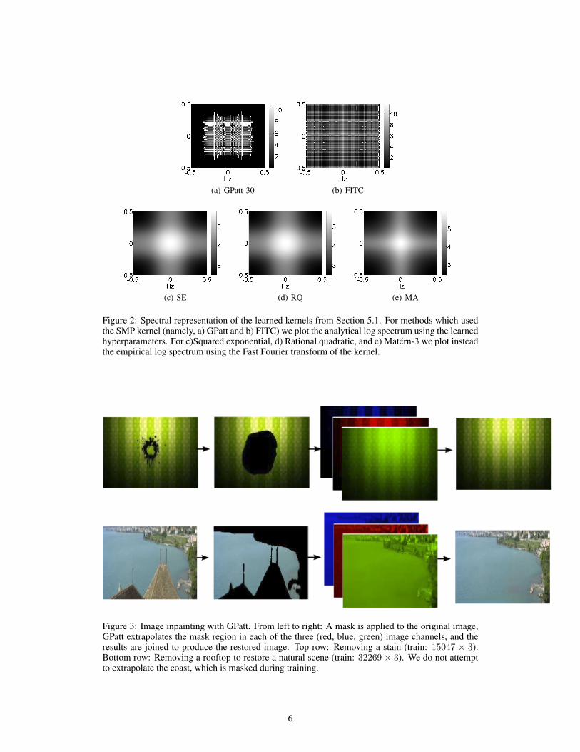
6 Spectrum Analysis

We can gain further insight into the behavior of GPatt by looking at the spectral density learned bythe spectral mixture kernel. Figure 2 shows the log spectrum representations of the learned kernelsfrom Section 5.1. Smoothers, such as the popular kernels SE, RQ, and MA, concentrate their spectralenergy around the origin, differing only by their support for higher frequencies. Methods which usedthe SMP kernel, such as the GPatt and FITC (with an SMP kernel), are able to learn meaningfulfeatures in the spectrum space.

7 Enlarged Inpainting Image

8 Tread Plate, Stress Test, and Video Images

Figure 4 illustrates the images used for the stress tests. In Figure 5, we provide the results for thelarge pore example. Finally, Figure 6 shows the true and predicted movie frames.

References[1] C.E. Rasmussen and Z. Ghahramani. Occam’s razor. In Neural Information Process Systems,

2001.[2] I. Murray and R.P. Adams. Slice sampling covariance hyperparameters in latent Gaussian mod-

els. In Advances in Neural Information Processing Systems, 2010.[3] C.E. Rasmussen and C.K.I. Williams. Gaussian processes for Machine Learning. The MIT

Press, 2006.[4] Y Saatchi. Scalable Inference for Structured Gaussian Process Models. PhD thesis, University

of Cambridge, 2011.

4

−40−2002040

(a) GPatt

−40

−20

0

20

40

(b) GP-SE

Figure 1: In each image, the first two rows are the last 12 months of training data, and the lasttwo rows are 12 month forecasts. Note that this is a true extrapolation problem: all 12 months areforecast at once (this is not a rolling forecast). a) GPatt, b) GP-SE.

5

(a) GPatt-30 (b) FITC

(c) SE (d) RQ (e) MA

Figure 2: Spectral representation of the learned kernels from Section 5.1. For methods which usedthe SMP kernel (namely, a) GPatt and b) FITC) we plot the analytical log spectrum using the learnedhyperparameters. For c)Squared exponential, d) Rational quadratic, and e) Matern-3 we plot insteadthe empirical log spectrum using the Fast Fourier transform of the kernel.

Figure 3: Image inpainting with GPatt. From left to right: A mask is applied to the original image,GPatt extrapolates the mask region in each of the three (red, blue, green) image channels, and theresults are joined to produce the restored image. Top row: Removing a stain (train: 15047 × 3).Bottom row: Removing a rooftop to restore a natural scene (train: 32269 × 3). We do not attemptto extrapolate the coast, which is masked during training.

6

(a) Rubber mat (b) Tread plate (c) Pores

(d) Wood (e) Chain mail

(f) Cone

Figure 4: Images used for stress tests in Section 5.2. Figures a) through e) show the textures usedin the accuracy comparison of Table 1. Figure e) is the cone image which was used for the runtimeanalysis shown in Figure 3a.

100 200 300 400 500 600 700 800

100

200

300

400

500

600

(a) Train100 200 300 400 500 600 700 800

100

200

300

400

500

600

(b) Learn

Figure 5: GPatt on a particularly large multidimensional dataset. a) Training region (383400 points),b) GPatt-10 reconstruction of the missing region.

7

Figure 6: Recovering 5 consecutive slices from a movie. All 5 slices are missing during training:this is not one step ahead forecasting. (Top row: true slices take from the middle of the movie.Bottom row: predicted slices using GPatt-20.

8