SAMPLING THEORY - Carnegie Mellon School of Computer Science
41
2/20/15 1 Copyright © 2002-2013 by Roger B. Dannenberg SAMPLING THEORY Representing continuous signals with discrete numbers Roger B. Dannenberg Professor of Computer Science, Art, and Music Carnegie Mellon University 1 ICM Week 3 Copyright © 2002-2013 by Roger B. Dannenberg ICM Week 3 2 010110 010100 011000 011011 000111 100100 011000 000010 101100 111010 000101 011010 111011 011100 000100 From analog to digital (and back)
Transcript of SAMPLING THEORY - Carnegie Mellon School of Computer Science
2/20/15
1
Copyright © 2002-2013 by Roger B. Dannenberg
SAMPLING THEORY Representing continuous signals with discrete numbers Roger B. Dannenberg Professor of Computer Science, Art, and Music Carnegie Mellon University
1 ICM Week 3
Copyright © 2002-2013 by Roger B. Dannenberg ICM Week 3 2
010110 010100 011000 011011 000111 100100 011000 000010 101100 111010 000101 011010 111011 011100 000100
From analog to digital (and back)
2/20/15
2
Copyright © 2002-2013 by Roger B. Dannenberg ICM Week 3 3
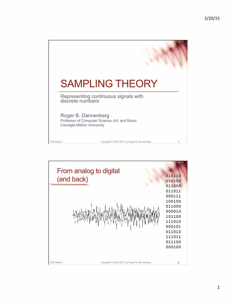
Analog to Digital Conversion Digital to Analog Conversion
010110 010100 011000 011011 000111
D to A A to D
Copyright © 2002-2013 by Roger B. Dannenberg ICM Week 3 4
Approach • Intuition • Frequency Domain (Fourier Transform) • Sampling Theory • Practical Results
2/20/15
3
Copyright © 2002-2013 by Roger B. Dannenberg ICM Week 3 5
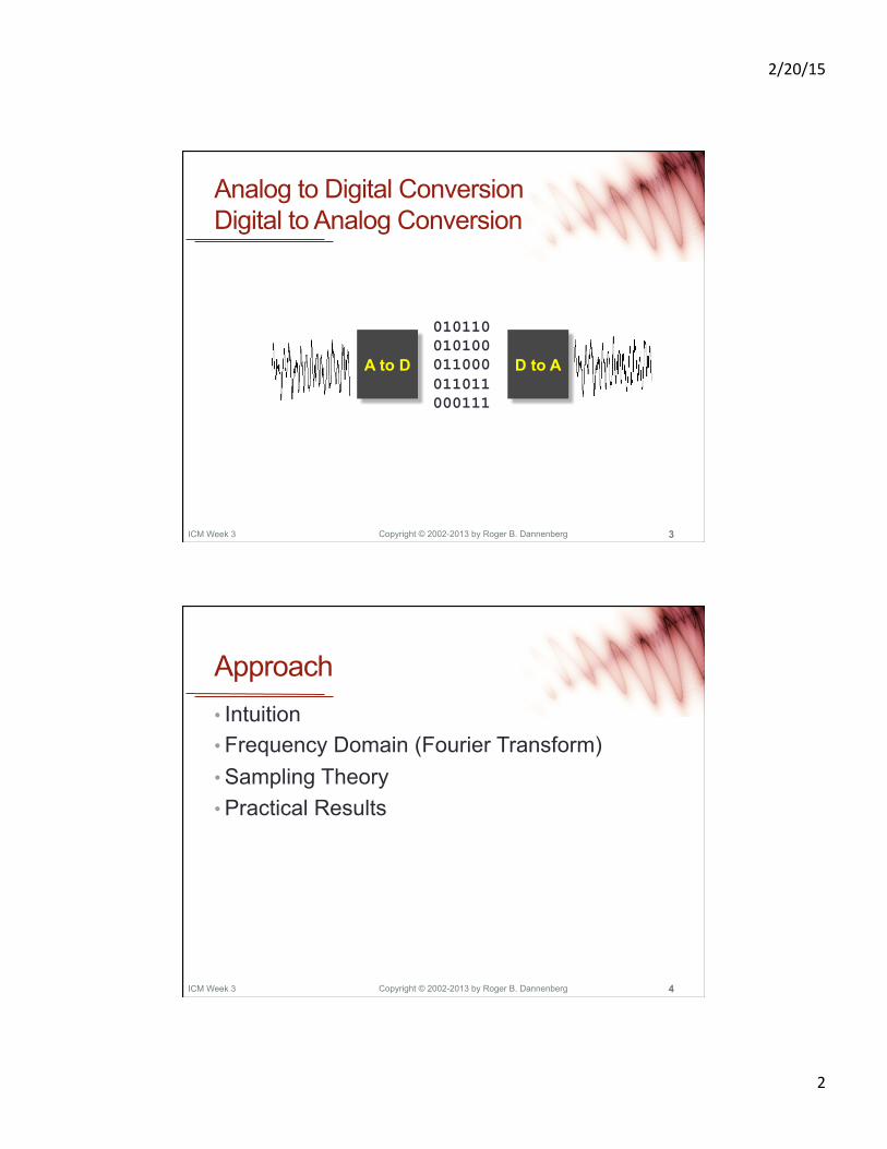
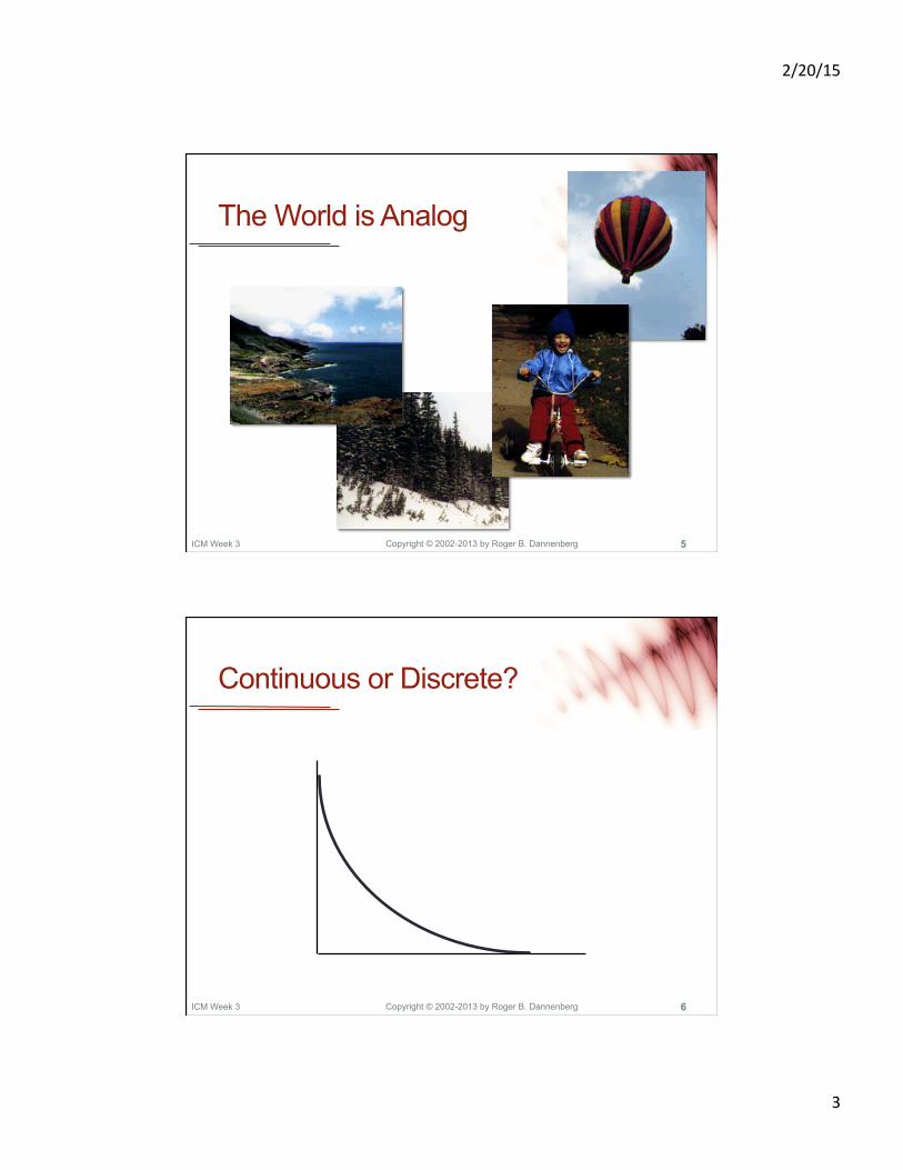
The World is Analog
Copyright © 2002-2013 by Roger B. Dannenberg ICM Week 3 6
Continuous or Discrete?

2/20/15
4
Copyright © 2002-2013 by Roger B. Dannenberg ICM Week 3 7
Discrete Amplitude (Y axis)
Copyright © 2002-2013 by Roger B. Dannenberg ICM Week 3 8
Discrete Time (X axis)
2/20/15
5
Copyright © 2002-2013 by Roger B. Dannenberg ICM Week 3 9
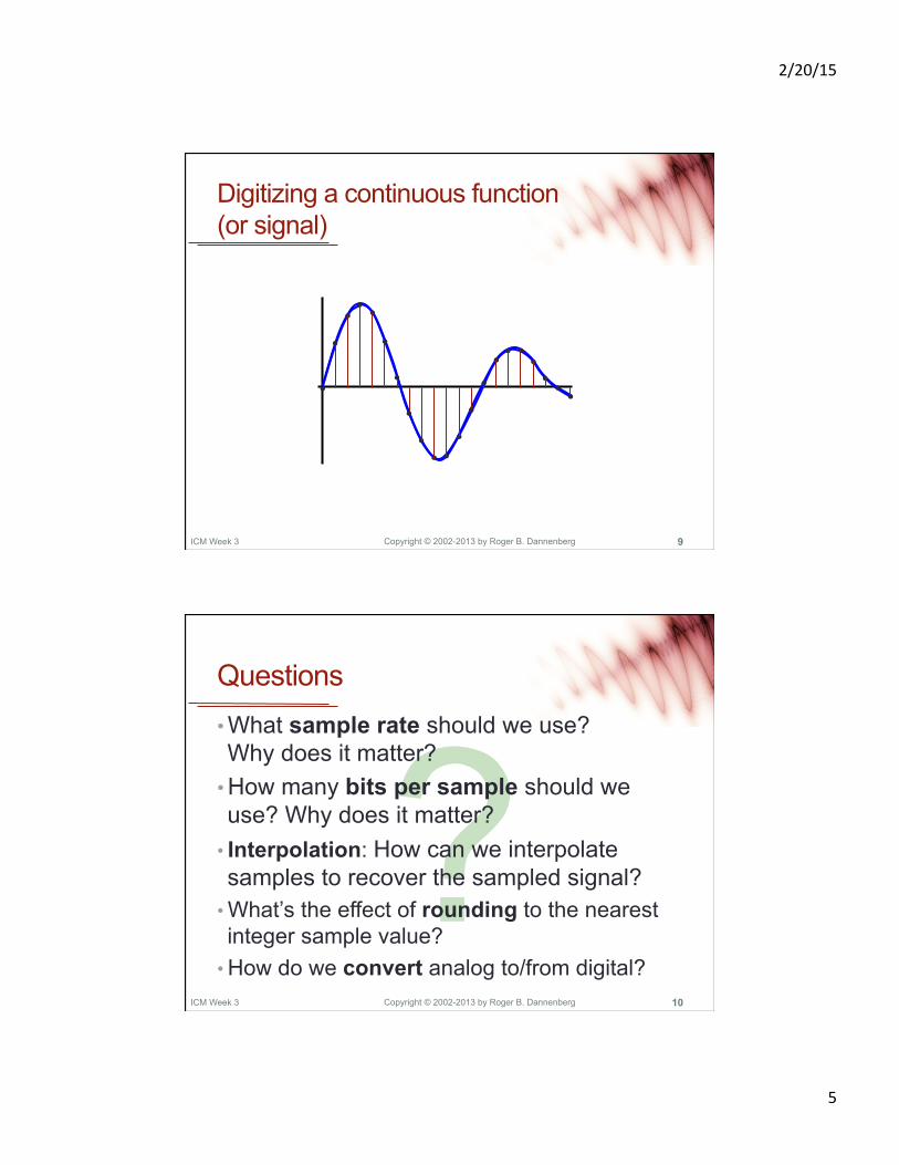
Digitizing a continuous function (or signal)
Copyright © 2002-2013 by Roger B. Dannenberg ICM Week 3 10
? Questions • What sample rate should we use? Why does it matter?
• How many bits per sample should we use? Why does it matter?
• Interpolation: How can we interpolate samples to recover the sampled signal?
• What’s the effect of rounding to the nearest integer sample value?
• How do we convert analog to/from digital?

2/20/15
6
Copyright © 2002-2013 by Roger B. Dannenberg ICM Week 3 11
Introduction to the Spectrum
Copyright © 2002-2013 by Roger B. Dannenberg ICM Week 3 12
Introduction to the Spectrum (2)
2/20/15
7
Copyright © 2002-2013 by Roger B. Dannenberg ICM Week 3 13
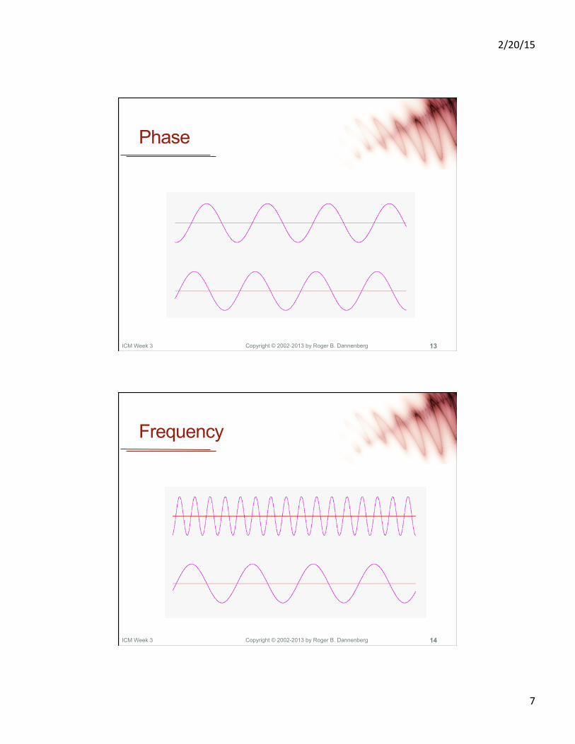
Phase
Copyright © 2002-2013 by Roger B. Dannenberg ICM Week 3 14
Frequency

2/20/15
8
Copyright © 2002-2013 by Roger B. Dannenberg ICM Week 3 15
Amplitude
Copyright © 2002-2013 by Roger B. Dannenberg ICM Week 3 16
Sinusoidal Partials
Amplitude A
Frequency ω
Phase φ
A ⋅sin(ωt +φ)

2/20/15
9
Copyright © 2002-2013 by Roger B. Dannenberg
Fourier Transform • Our goal is to transform a function-of-time representation of a signal to a function-of-frequency representation
• Express the time function as an (infinite) sum of sinusoids.
• Express the infinite sum as a function from frequency to amplitude
• I.e. for each frequency, what is the amplitude of the sinusoid of that frequency within this infinite sum?
ICM Week 3 17
Copyright © 2002-2013 by Roger B. Dannenberg ICM Week 3 18
Fourier Transform: Cartesian Coordinates
R(ω) = f (t)cosωt dt−∞
∞
∫
X(ω) = − f (t)sinωt dt−∞
∞
∫
Real part:
Imaginary part:

2/20/15
10
Copyright © 2002-2013 by Roger B. Dannenberg
What About Phase? • Remember at each frequency, we said there is one sinusoidal component: • A is amplitude • ω is frequency • φ is phase
• The Fourier analysis computes two amplitudes: • R(ω) and X(ω) • Trig identities tell us there is no conflict:
ICM Week 3 19
A = R2 + X 2 φ = arctan(X / R)
A ⋅sin(ωt +φ)
A(ω) = R2 (ω)+ X 2 (ω) φ(ω) = arctan(X(ω) / R(ω))
Copyright © 2002-2013 by Roger B. Dannenberg
From Cartesian to Complex • R is “real” or cosine part • X is “imaginary” or sine part • Use
ICM Week 3 20
F(ω) = R(ω)+ j ⋅X(ω)
2/20/15
11
Copyright © 2002-2013 by Roger B. Dannenberg
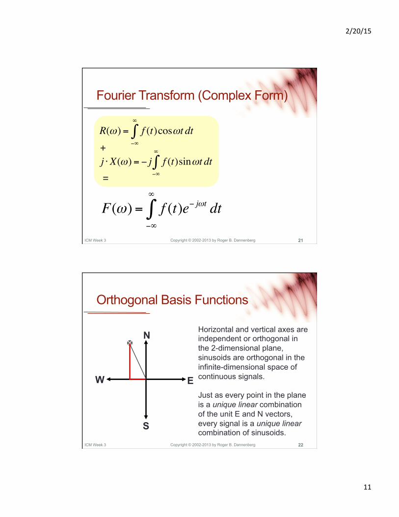
Fourier Transform (Complex Form)
ICM Week 3 21
F(ω) = f (t)e− jωt dt−∞
∞
∫
R(ω) = f (t)cosωt dt−∞
∞
∫
j ⋅X(ω) = − j f (t)sinωt dt−∞
∞
∫+
=
Copyright © 2002-2013 by Roger B. Dannenberg ICM Week 3 22
Orthogonal Basis Functions
N
E
S
W
Horizontal and vertical axes are independent or orthogonal in the 2-dimensional plane, sinusoids are orthogonal in the infinite-dimensional space of continuous signals. Just as every point in the plane is a unique linear combination of the unit E and N vectors, every signal is a unique linear combination of sinusoids.
2/20/15
12
Copyright © 2002-2013 by Roger B. Dannenberg ICM Week 3 23
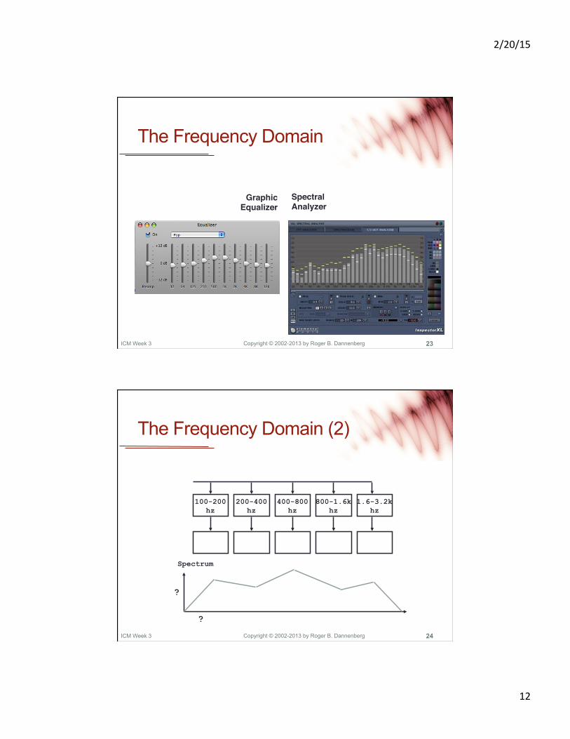
The Frequency Domain
Graphic!Equalizer!
Spectral!Analyzer
Copyright © 2002-2013 by Roger B. Dannenberg ICM Week 3 24
The Frequency Domain (2)
100-200 hz
200-400 hz
400-800 hz
800-1.6k hz
1.6-3.2k hz
Spectrum
?
?
2/20/15
13
Copyright © 2002-2013 by Roger B. Dannenberg ICM Week 3 25
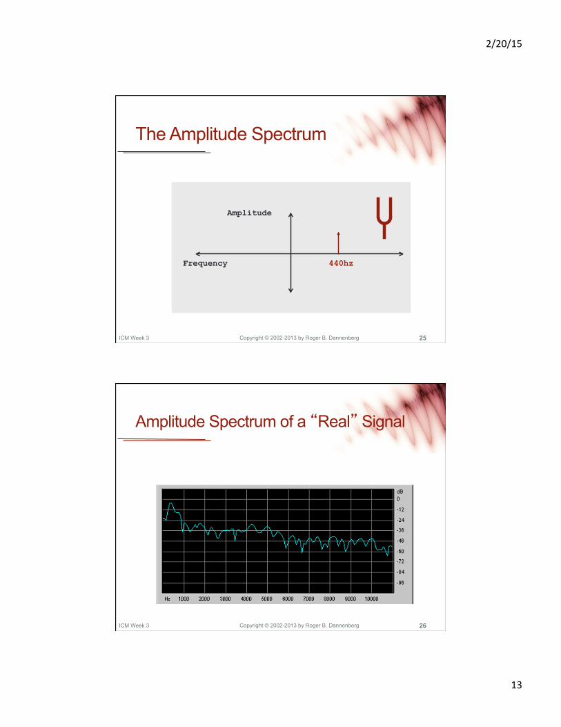
The Amplitude Spectrum
Amplitude
Frequency 440hz
Copyright © 2002-2013 by Roger B. Dannenberg ICM Week 3 26
Amplitude Spectrum of a “Real” Signal

2/20/15
14
Copyright © 2002-2013 by Roger B. Dannenberg
Representations • (Real, Imaginary) or (Amplitude, Phase)?
• Power ~ Amplitude2
• We generally cannot hear phase • Measure a stationary signal after Δt: Amplitude
spectrum is unchanged, but phase changes by • Given (amplitude, phase)
• It’s hard to plot both • Usually, we ignore the phase
ICM Week 3 27
Δt ⋅ω
Copyright © 2002-2013 by Roger B. Dannenberg
Time vs Frequency • What happens to time when you transform to the frequency domain?
• Note that time is “integrated out” • NO TIME REMAINS • The Fourier Transform of a signal is not a function of time !!!!!
• (Later, we’ll look at short-time transforms – e.g. what you see on a time-varying spectral display – which are time varying.)
ICM Week 3 28
F(ω) = f (t)e− jωt dt−∞
∞
∫

2/20/15
15
Copyright © 2002-2013 by Roger B. Dannenberg
PERFECT SAMPLING From continuous signals to discrete samples and back again
ICM Week 3 29
Copyright © 2002-2013 by Roger B. Dannenberg
Sampling – Time Domain • What happens when you sample a signal? • In time domain, multiplication by a pulse train:
ICM Week 3 30
✕
=
time
time
time
2/20/15
16
Copyright © 2002-2013 by Roger B. Dannenberg
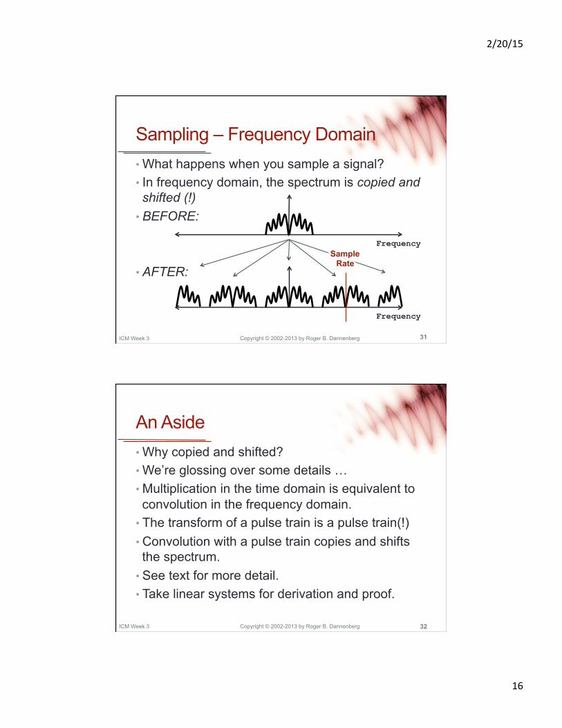
Sampling – Frequency Domain • What happens when you sample a signal? • In frequency domain, the spectrum is copied and shifted (!)
• BEFORE:
• AFTER:
ICM Week 3 31
Frequency
Frequency Sample
Rate
Copyright © 2002-2013 by Roger B. Dannenberg
An Aside • Why copied and shifted? • We’re glossing over some details … • Multiplication in the time domain is equivalent to convolution in the frequency domain.
• The transform of a pulse train is a pulse train(!) • Convolution with a pulse train copies and shifts the spectrum.
• See text for more detail. • Take linear systems for derivation and proof.
ICM Week 3 32
2/20/15
17
Copyright © 2002-2013 by Roger B. Dannenberg ICM Week 3 33
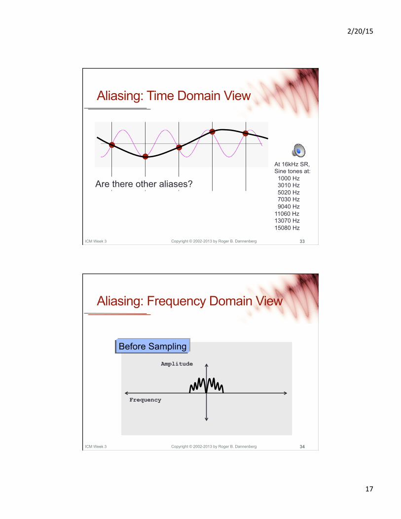
Aliasing: Time Domain View
Are there other aliases?
At 16kHz SR, Sine tones at: 1000 Hz 3010 Hz 5020 Hz 7030 Hz 9040 Hz 11060 Hz 13070 Hz 15080 Hz
Copyright © 2002-2013 by Roger B. Dannenberg ICM Week 3 34
Aliasing: Frequency Domain View
Amplitude
Frequency
Before Sampling

2/20/15
18
Copyright © 2002-2013 by Roger B. Dannenberg ICM Week 3 35
Frequency Domain View (2)
Amplitude
Frequency
After Sampling
Sample Rate
Copyright © 2002-2013 by Roger B. Dannenberg ICM Week 3 36
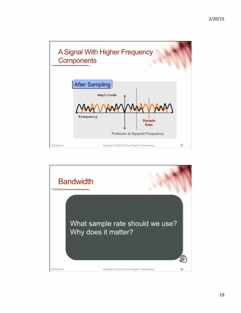
A Signal With Higher Frequency Components
Amplitude
Frequency
Before Sampling
2/20/15
19
Copyright © 2002-2013 by Roger B. Dannenberg ICM Week 3 37
A Signal With Higher Frequency Components
Amplitude
Frequency
After Sampling
Sample Rate
Foldover at Nyquist Frequency
Copyright © 2002-2013 by Roger B. Dannenberg
Bandwidth
ICM Week 3 38
What sample rate should we use? Why does it matter?
2/20/15
20
Copyright © 2002-2013 by Roger B. Dannenberg
Bandwidth
ICM Week 3 39
Copyright © 2002-2013 by Roger B. Dannenberg ICM Week 3 40
Sampling Without Aliasing
S/H A/D
Prefilter Sample
and Hold
Analog to
Digital
Prefilter removes all frequencies above 1/2 sampling rate (the Nyquist Frequency)
How do we convert analog to/from digital?
2/20/15
21
Copyright © 2002-2013 by Roger B. Dannenberg ICM Week 3 41
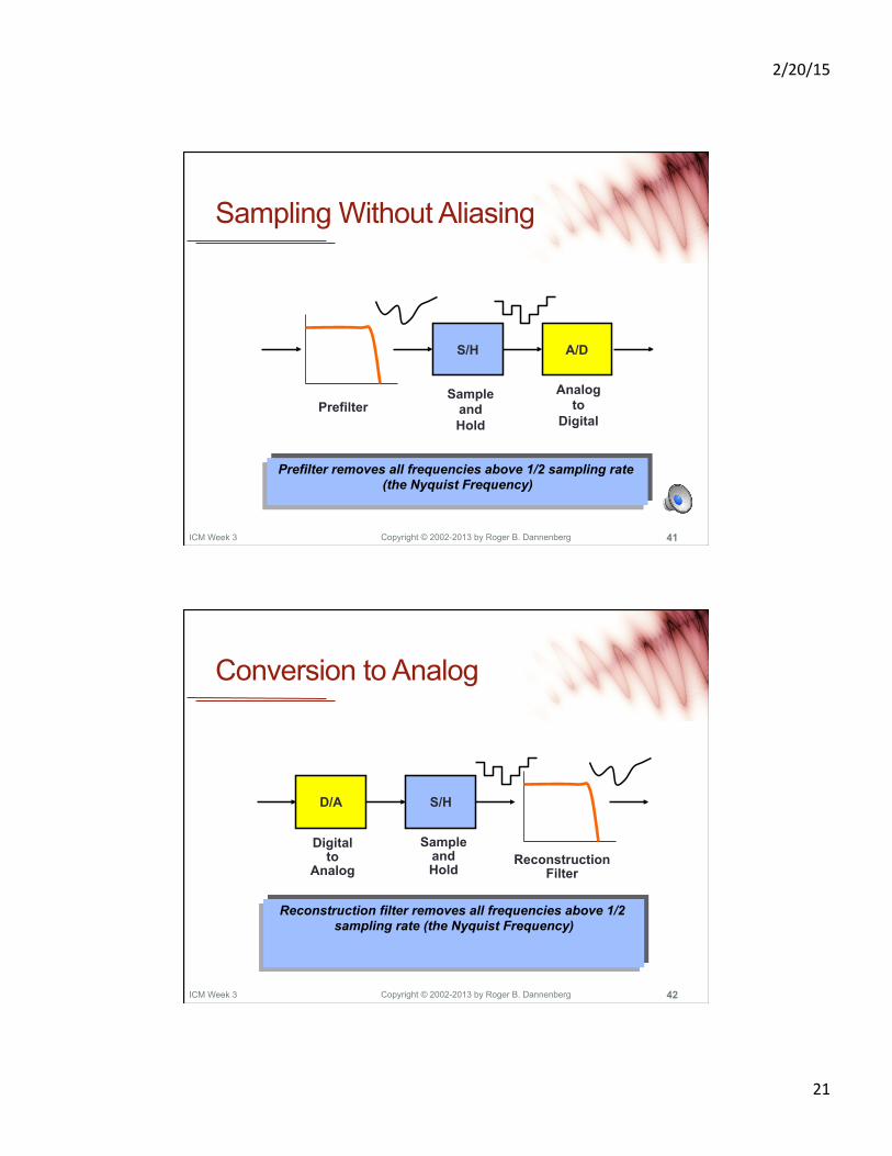
Sampling Without Aliasing
S/H A/D
Prefilter Sample
and Hold
Analog to
Digital
Prefilter removes all frequencies above 1/2 sampling rate (the Nyquist Frequency)
Copyright © 2002-2013 by Roger B. Dannenberg ICM Week 3 42
Conversion to Analog
Reconstruction Filter
S/H
Sample and Hold
D/A
Digital to
Analog
Reconstruction filter removes all frequencies above 1/2 sampling rate (the Nyquist Frequency)
2/20/15
22
Copyright © 2002-2013 by Roger B. Dannenberg ICM Week 3 43
What Does a Sample “Mean”?
Copyright © 2002-2013 by Roger B. Dannenberg ICM Week 3 44
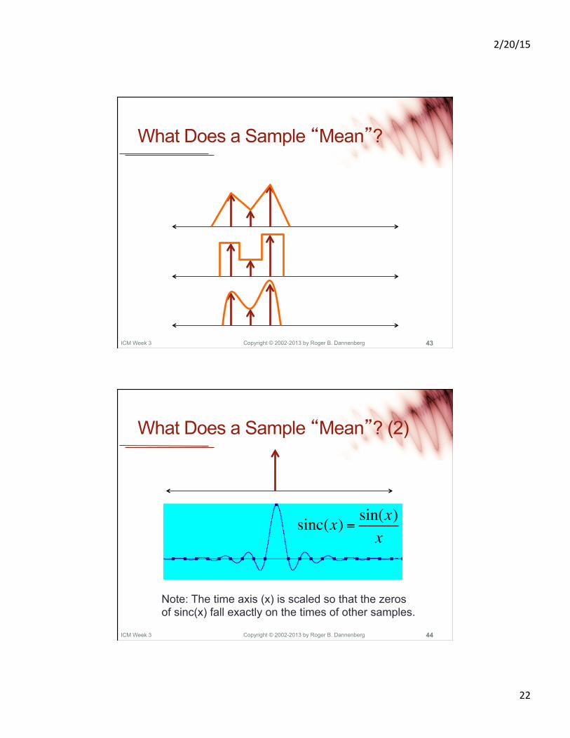
What Does a Sample “Mean”? (2)
sinc(x) = sin(x)x
Note: The time axis (x) is scaled so that the zeros of sinc(x) fall exactly on the times of other samples.
2/20/15
23
Copyright © 2002-2013 by Roger B. Dannenberg ICM Week 3 45
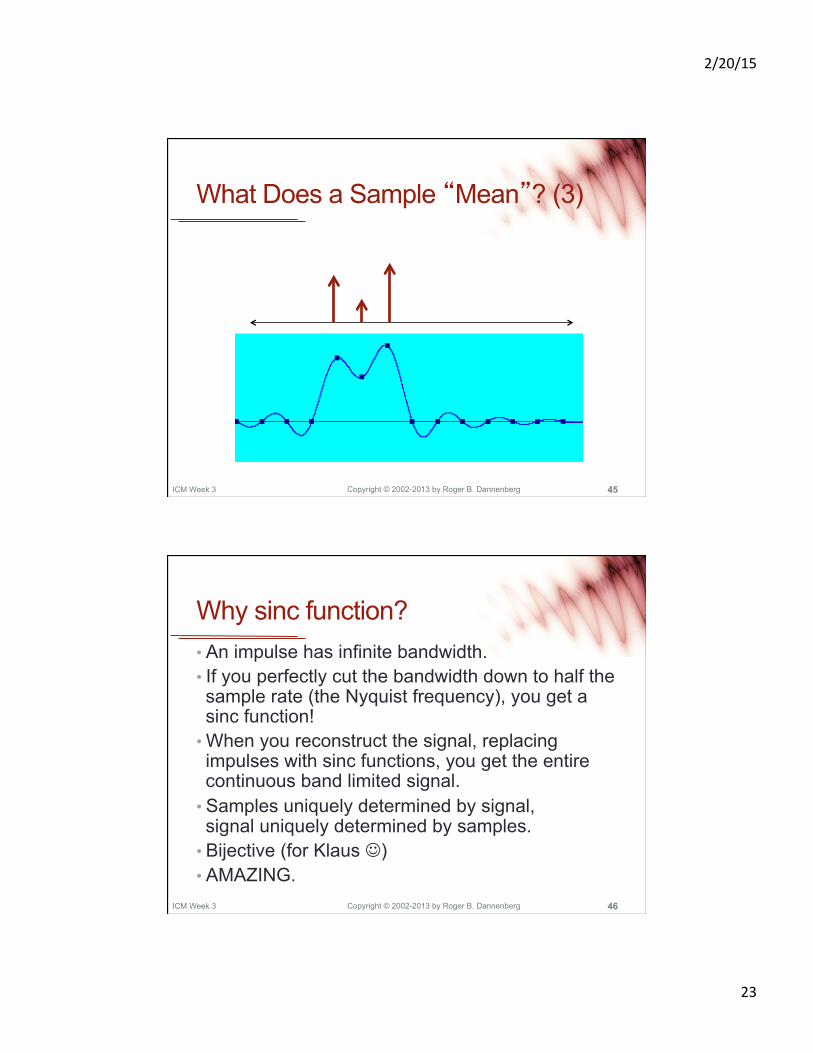
What Does a Sample “Mean”? (3)
Copyright © 2002-2013 by Roger B. Dannenberg
Why sinc function? • An impulse has infinite bandwidth. • If you perfectly cut the bandwidth down to half the sample rate (the Nyquist frequency), you get a sinc function!
• When you reconstruct the signal, replacing impulses with sinc functions, you get the entire continuous band limited signal.
• Samples uniquely determined by signal, signal uniquely determined by samples.
• Bijective (for Klaus ) • AMAZING.
ICM Week 3 46
2/20/15
24
Copyright © 2002-2013 by Roger B. Dannenberg
Interpolation/Reconstruction • Convolve with a sinc function • In other words, form the superposition of sinc functions shifted by the sample times and scaled by the sample values.
• Requires infinite lookahead and infinite computation!
• But sinc decays as 1/time, so good approximations are expensive but at least possible.
ICM Week 3 47
How can we interpolate samples to recover the sampled signal?
Copyright © 2002-2013 by Roger B. Dannenberg
Interpolation/Reconstruction • Convolve with a sinc function • In other words, form the superposition of sinc functions shifted by the sample times and scaled by the sample values.
• Requires infinite lookahead and infinite computation!
• But sinc decays as 1/time, so good approximations are expensive but at least possible.
ICM Week 3 48
2/20/15
25
Copyright © 2002-2013 by Roger B. Dannenberg
IMPERFECT SAMPLING What is the impact of errors and rounding?
ICM Week 3 49
Copyright © 2002-2013 by Roger B. Dannenberg ICM Week 3 50
How to Describe Noise • Since absolute levels rarely exist, measure RATIO of Signal to Noise.
• Since signal level is variable, measure MAXIMUM Signal to Noise.
• Units: dB = decibel 10dB = ×10 power 20dB = ×100 power = ×10 amplitude 6dB = ×2 amplitude

2/20/15
26
Copyright © 2002-2013 by Roger B. Dannenberg ICM Week 3 51
Quantization Noise
Signal""
Quantization Error"
To simplify analysis, assume quantization error is uniformly randomly distributed in [-0.5, +0.5]!
Copyright © 2002-2013 by Roger B. Dannenberg
Quantization Examples
ICM Week 3 52
Sine Tone Cello
16-bit
8-bit
4-bit
2-bit

2/20/15
27
Copyright © 2002-2013 by Roger B. Dannenberg
Quantization Noise, M bits/sample • Rounding effects can be approximated by adding white noise (uniform random samples) of maximum amplitude of ½ least significant bit.
ICM Week 3 53
SNR(dB) = 6.02M + 1.76 (about 6dB/bit)
What’s the effect of rounding to the nearest integer sample value?
Copyright © 2002-2013 by Roger B. Dannenberg
Quantization Noise, M bits/sample • Rounding effects can be approximated by adding white noise (uniform random samples) of maximum amplitude of ½ least significant bit.
ICM Week 3 54
SNR(dB) = 6.02M + 1.76 (about 6dB/bit)

2/20/15
28
Copyright © 2002-2013 by Roger B. Dannenberg ICM Week 3 55
Noise
How many bits per sample should we use? Why does it matter?
Copyright © 2002-2013 by Roger B. Dannenberg ICM Week 3 56
Noise
2/20/15
29
Copyright © 2002-2013 by Roger B. Dannenberg ICM Week 3 57
Can Discrete Samples Really Capture a Continuous Signal?
• Band-limited signal no lost frequencies! • To the extent you can do perfect sampling no noise!
DISCRETE SAMPLES CAN CAPTURE A CONTINUOUS
BAND-LIMITED SIGNAL WITHOUT LOSS
Copyright © 2002-2013 by Roger B. Dannenberg
Summary • Theoretical result: discrete samples can capture all information in a band-limited signal!
• Practical result 1: sampling limits bandwidth to 1/2 sampling rate (the Nyquist frequency)
• Practical result 2: sampling adds quantization noise; SNR is about 6dB per bit
• What’s a decibel?
ICM Week 3 58
2/20/15
30
Copyright © 2002-2013 by Roger B. Dannenberg
DITHER AND OVERSAMPLING Additional techniques for practical digital audio
ICM Week 3 59
Copyright © 2002-2013 by Roger B. Dannenberg ICM Week 3 60
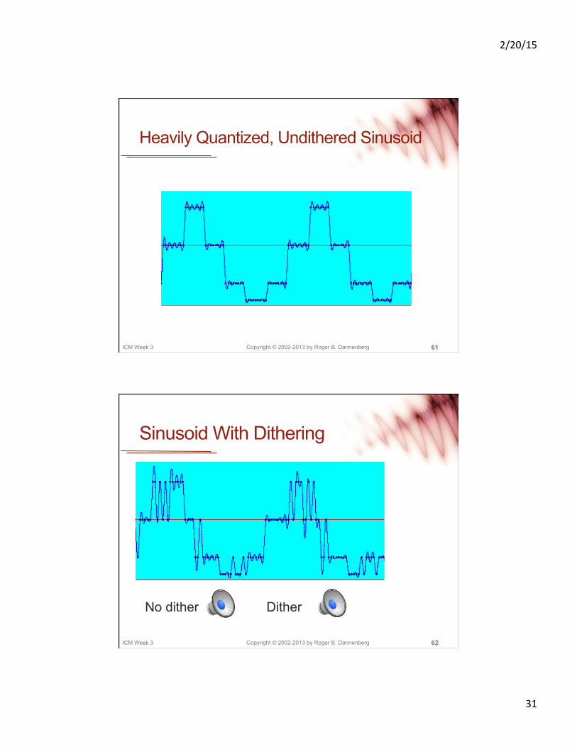
Dither • Sometimes rounding error is correlated to signal. • Add analog noise prior to quantization to decorrelate rounding.
• Typically, noise has peak-to-peak amplitude of one quantization step.
2/20/15
31
Copyright © 2002-2013 by Roger B. Dannenberg ICM Week 3 61
Heavily Quantized, Undithered Sinusoid
Copyright © 2002-2013 by Roger B. Dannenberg ICM Week 3 62
Sinusoid With Dithering
No dither Dither
2/20/15
32
Copyright © 2002-2013 by Roger B. Dannenberg ICM Week 3 63
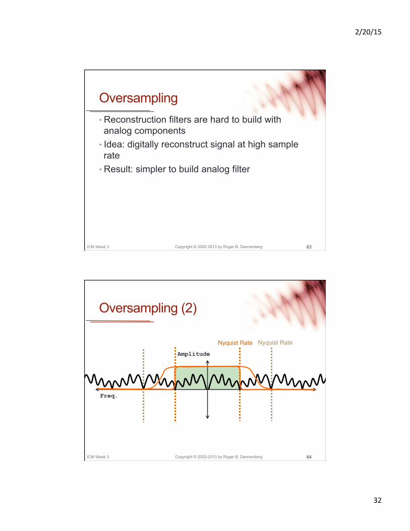
Oversampling • Reconstruction filters are hard to build with analog components
• Idea: digitally reconstruct signal at high sample rate
• Result: simpler to build analog filter
Copyright © 2002-2013 by Roger B. Dannenberg ICM Week 3 64
Oversampling (2)
Amplitude
Freq.
Nyquist Rate"Nyquist Rate"
2/20/15
33
Copyright © 2002-2013 by Roger B. Dannenberg
THE FREQUENCY DOMAIN An alternative to waveforms (the time domain)
ICM Week 3 65
Copyright © 2002-2013 by Roger B. Dannenberg
The Frequency Domain • Examples of Simple Spectra • Fourier Transform vs Short-Term Fourier Transform
• DFT – Discrete Fourier Transform • FFT – Fast Fourier Transform • Windowing
ICM Week 3 66

2/20/15
34
Copyright © 2002-2013 by Roger B. Dannenberg
Formal Definition
ICM Week 3 67
R(ω) = f (t)cosωt dt−∞
∞
∫
X(ω) = − f (t)sinωt dt−∞
∞
∫
F(ω) = f (t)e− jωt dt−∞
∞
∫
Copyright © 2002-2013 by Roger B. Dannenberg
Simple Spectra Examples • Sinusoid
• Noise
• Tone with harmonics
ICM Week 3 68
2/20/15
35
Copyright © 2002-2013 by Roger B. Dannenberg
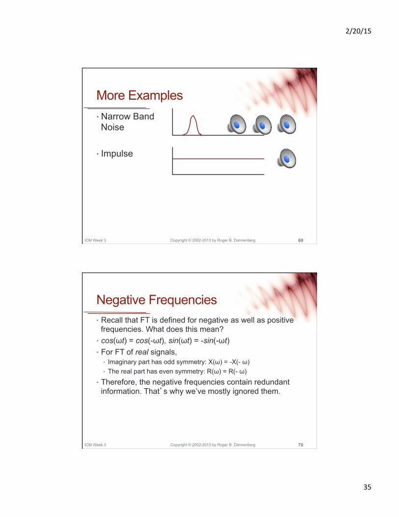
More Examples • Narrow Band Noise
• Impulse
ICM Week 3 69
Copyright © 2002-2013 by Roger B. Dannenberg
Negative Frequencies • Recall that FT is defined for negative as well as positive
frequencies. What does this mean? • cos(ωt) = cos(-ωt), sin(ωt) = -sin(-ωt) • For FT of real signals,
• Imaginary part has odd symmetry: X(ω) = -X(- ω) • The real part has even symmetry: R(ω) = R(- ω)
• Therefore, the negative frequencies contain redundant information. That’s why we’ve mostly ignored them.
ICM Week 3 70
2/20/15
36
Copyright © 2002-2013 by Roger B. Dannenberg
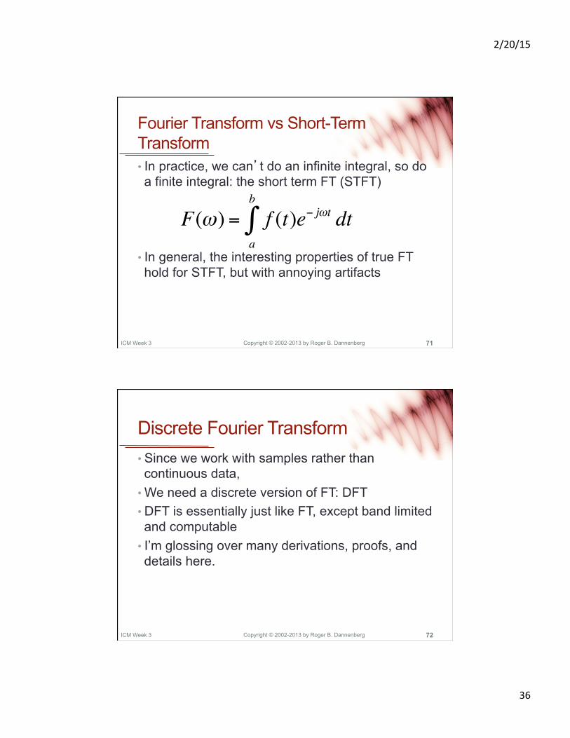
Fourier Transform vs Short-Term Transform • In practice, we can’t do an infinite integral, so do a finite integral: the short term FT (STFT)
• In general, the interesting properties of true FT hold for STFT, but with annoying artifacts
ICM Week 3 71
F(ω) = f (t)e− jωt dta
b
∫
Copyright © 2002-2013 by Roger B. Dannenberg
Discrete Fourier Transform • Since we work with samples rather than continuous data,
• We need a discrete version of FT: DFT • DFT is essentially just like FT, except band limited and computable
• I’m glossing over many derivations, proofs, and details here.
ICM Week 3 72

2/20/15
37
Copyright © 2002-2013 by Roger B. Dannenberg
Fast Fourier Transform • Replacing integral with a sum, you would think computing R(ω) would be an O(n2) problem
• Interestingly, there is an O(n log n) algorithm, the Fast Fourier Transform, or FFT
ICM Week 3 73
Fk = fne− j2πkn/N
n=a
b
∑
Copyright © 2002-2013 by Roger B. Dannenberg
Windowing • Typically, you can reduce the artifacts of the STFT by windowing:
• Different windows optimize different criteria: Hamming, Hanning, Blackman, etc.
ICM Week 3 74

2/20/15
38
Copyright © 2002-2013 by Roger B. Dannenberg
More Examples Using Audacity
ICM Week 3 75
Copyright © 2002-2013 by Roger B. Dannenberg
AMPLITUDE MODULATION Synthesis techniques based on signal multiplication
ICM Week 3 76
2/20/15
39
Copyright © 2002-2013 by Roger B. Dannenberg
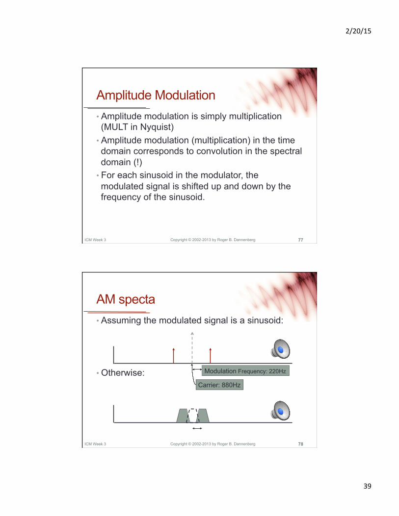
Amplitude Modulation • Amplitude modulation is simply multiplication (MULT in Nyquist)
• Amplitude modulation (multiplication) in the time domain corresponds to convolution in the spectral domain (!)
• For each sinusoid in the modulator, the modulated signal is shifted up and down by the frequency of the sinusoid.
ICM Week 3 77
Copyright © 2002-2013 by Roger B. Dannenberg
AM specta • Assuming the modulated signal is a sinusoid:
• Otherwise:
ICM Week 3 78
Carrier: 880Hz
Modulation Frequency: 220Hz

2/20/15
40
Copyright © 2002-2013 by Roger B. Dannenberg
Ring Modulation • Ring Modulation is named after the “ring modulator,” an analog approach to signal multiplication.
• See code_3.htm for AM examples
ICM Week 3 79
Copyright © 2002-2013 by Roger B. Dannenberg
Constant Offset • What is the difference between: lfo(6)
• And 2 + lfo(6)
• ?
ICM Week 3 80
2/20/15
41
Copyright © 2002-2013 by Roger B. Dannenberg
Summary • Dithering sometimes used to avoid quantization artifacts
• Oversampling is standard technique to move (some) filtering to the digital domain
• Amplitude Modulation by a sinusoid shifts the spectrum up and down by the frequency of the modulator
ICM Week 3 81