Capacity Value of Concentrating Solar Power Plants · Office of Scientific and Technical...
49
NREL is a national laboratory of the U.S. Department of Energy, Office of Energy Efficiency & Renewable Energy, operated by the Alliance for Sustainable Energy, LLC. Contract No. DE-AC36-08GO28308 Capacity Value of Concentrating Solar Power Plants Seyed Hossein Madaeni and Ramteen Sioshansi Ohio State University Paul Denholm National Renewable Energy Laboratory Technical Report NREL/TP-6A20-51253 June 2011
Transcript of Capacity Value of Concentrating Solar Power Plants · Office of Scientific and Technical...
NREL is a national laboratory of the US Department of Energy Office of Energy Efficiency amp Renewable Energy operated by the Alliance for Sustainable Energy LLC
Contract No DE-AC36-08GO28308
Capacity Value of Concentrating Solar Power Plants Seyed Hossein Madaeni and Ramteen Sioshansi Ohio State University
Paul Denholm National Renewable Energy Laboratory
Technical Report NRELTP-6A20-51253 June 2011
NREL is a national laboratory of the US Department of Energy Office of Energy Efficiency amp Renewable Energy operated by the Alliance for Sustainable Energy LLC
National Renewable Energy Laboratory 1617 Cole Boulevard Golden Colorado 80401 303-275-3000 bull wwwnrelgov
Contract No DE-AC36-08GO28308
Capacity Value of Concentrating Solar Power Plants Seyed Hossein Madaeni and Ramteen Sioshansi Ohio State University
Paul Denholm National Renewable Energy Laboratory
Prepared under Task No SS101410
Technical Report NRELTP-6A20-51253 June 2011
NOTICE
This report was prepared as an account of work sponsored by an agency of the United States government Neither the United States government nor any agency thereof nor any of their employees makes any warranty express or implied or assumes any legal liability or responsibility for the accuracy completeness or usefulness of any information apparatus product or process disclosed or represents that its use would not infringe privately owned rights Reference herein to any specific commercial product process or service by trade name trademark manufacturer or otherwise does not necessarily constitute or imply its endorsement recommendation or favoring by the United States government or any agency thereof The views and opinions of authors expressed herein do not necessarily state or reflect those of the United States government or any agency thereof
Available electronically at httpwwwostigovbridge
Available for a processing fee to US Department of Energy and its contractors in paper from
US Department of Energy Office of Scientific and Technical Information
PO Box 62 Oak Ridge TN 37831-0062 phone 8655768401 fax 8655765728 email mailtoreportsadonisostigov
Available for sale to the public in paper from
US Department of Commerce National Technical Information Service 5285 Port Royal Road Springfield VA 22161 phone 8005536847 fax 7036056900 email ordersntisfedworldgov online ordering httpwwwntisgovhelpordermethodsaspx
Cover Photos (left to right) PIX 16416 PIX 17423 PIX 16560 PIX 17613 PIX 17436 PIX 17721
Printed on paper containing at least 50 wastepaper including 10 post consumer waste
iii
Acknowledgments
The authors would like to thank Adam Green Michael Milligan Mark Mehos Robin Newmark Walter Short and Craig Turchi for helpful discussions and suggestions
iv
List of Acronyms
APS Arizona Public Service CSP concentrating solar power EFOR expected forced outage rate EIA US Department of Energyrsquos Energy Information
Administration ELCC effective load carrying capability ERCOT Electric Reliability Council of Texas FCA forward capacity auction FCM forward capacity market FERC Federal Energy Regulatory Commission GADS Generating Availability Data System HTF heat transfer fluid ISO Independent System Operator LOLE loss of load expectation LOLP loss of load probability LSE load-serving entity MIP mixed-integer program MW-e megawatts of electricity NERC North American Electric Reliability Corporation NP Nevada Power PHS pumped hydroelectric storage PV photovoltaic SAM Solar Advisor Model SM solar multiple TES thermal energy storage WECC Western Electricity Coordinating Council
v
Executive Summary
This study estimates the capacity value of a concentrating solar power (CSP) plant at a variety of locations within the western United States This is done by optimizing the operation of the CSP plant and by using the effective load carrying capability (ELCC) metric which is a standard reliability-based capacity value estimation technique Although the ELCC metric is the most accurate estimation technique we show that a simpler capacity-factor-based approximation method can closely estimate the ELCC value
Without storage the capacity value of CSP plants varies widely depending on the year and solar multiple The average capacity value of plants evaluated ranged from 45ndash90 with a solar multiple range of 10ndash15 When introducing thermal energy storage (TES) the capacity value of the CSP plant is more difficult to estimate since one must account for energy in storage We apply a capacity-factor-based technique under two different market settings an energy-only market and an energy and capacity market Our results show that adding TES to a CSP plant can increase its capacity value significantly at all of the locations Adding a single hour of TES significantly increases the capacity value above the no-TES case and with four hours of storage or more the average capacity value at all locations exceeds 90
vi
Table of ContentsList of Figures vii List of Tables viii 1 Introduction 1 2 Methods for Estimating Capacity Value 2
21 Effective Load Carrying Capability 222 Approximation Methods 4
221 Highest-Load Hours Approximation Method 5222 Highest Loss of Load Probability Hours Approximation Method 5223 Loss-of-Load-Probability-Weighted Highest-Load Hours Approximation Method 5
3 Concentrating Solar Power Model 6 4 Data Requirements 10 5 Capacity Value of a Concentrating Solar Power Plant without Thermal Energy Storage 12
51 Effect of Expected Forced Outage Rates on Concentrating Solar Power Capacity Value 2152 Effect of Load Errors on Concentrating Solar Power Capacity Value 2253 Effect of Sub-Hourly Variability on Concentrating Solar Power Capacity Value 23
6 Capacity Value of a Concentrating Solar Power Plant with Thermal Energy Storage 25
61 Capacity Value of a Concentrating Solar Power Plant with Thermal Energy Storage in an Energy-Only Market 26
62 Capacity Value of a Concentrating Solar Power Plant with Thermal Energy Storage in a Capacity Market 32621 Capacity Market Procedures 32622 Optimization Model 33623 Results 34
7 Conclusions 38 References 39
vii
List of Figures
Figure 1 Schematic of a parabolic trough CSP plant with TES 6 Figure 2 Average annual capacity value of a CSP plant with no TES in different locations 13 Figure 3 Annual capacity value of a CSP plant with no TES at the New Mexico location 14 Figure 4 Hourly LOLPs and dispatch of a CSP plant with no TES at the New Mexico location
with an SM of 10 on August 1 2000 15 Figure 5 Hourly loads and solar radiation at the New Mexico location on August 1 2000 15 Figure 6 Hourly LOLPs and dispatch of a CSP plan with no TES at the New Mexico location
with an SM of 10 on August 10 2004 16 Figure 7 Hourly loads and solar radiation at the New Mexico location on August 10 2004 16 Figure 8 Annual average capacity value of a CSP plant with no TES at the Imperial Valley
location using the ELCC metric and approximation techniques that select the top 10 hours 17
Figure 9 Annual average capacity value of a CSP plant with no TES at the Imperial Valley location using the ELCC metric and approximation techniques that select the top 100 hours 18
Figure 10 Annual average capacity value of a CSP plant with no TES at the Imperial Valley location using the ELCC metric and approximation techniques that select the top 10 of hours 18
Figure 11 Annual average capacity value of a CSP plant with no TES at the New Mexico location using the ELCC metric and approximation techniques that select the top 10 hours 19
Figure 12 Annual average capacity value of a CSP plant with no TES at the Death Valley location using the ELCC metric and approximation techniques that select the top 10 hours 20
Figure 13 Annual average capacity value of a CSP plant with no TES at the Nevada location using the ELCC metric and approximation techniques that select the top 10 hours 20
Figure 14 Annual average capacity value of a CSP plant with no TES at the Arizona location using the ELCC metric and approximation techniques that select the top 10 hours 21
Figure 15 Average annual capacity value of a CSP plant with no TES at the Imperial Valley location based on ELCC metric with constant and varying conventional generator characteristics 22
Figure 16 Average annual capacity value of a CSP plant with no TES at the Imperial Valley location based on ELCC metric with loads shifted 23
Figure 17 Capacity value of a CSP plant with no TES at the Boulder City Nevada location based on ELCC metric while using hourly and one-minute interval solar data 24
Figure 18 Average annual capacity value of a CSP plant with TES at the Imperial Valley location under an energy-only market setting 27
Figure 19 Average annual capacity value of a CSP plant with TES at the New Mexico location under an energy-only market setting 27
Figure 20 Average annual capacity value of a CSP plant with TES at the Death Valley location under an energy-only market setting 28
Figure 21 Average annual capacity value of a CSP plant with TES at the Nevada location under an energy-only market setting 28
viii
Figure 22 Average annual capacity value of a CSP plant with TES at the Arizona location under an energy-only market setting 29
Figure 23 LOLP energy from solar field and energy in storage for a CSP plant at the Nevada location with four hours of TES and different SM values on July 12 1999 30
Figure 24 LOLP versus energy price for the Death Valley location in year 1999 31 Figure 25 LOLP energy from solar field and energy in storage for a CSP plant at the Death
Valley location with an SM of 27 and different TES sizes on July 12 1999 31 Figure 26 Average annual capacity value of a CSP plant with TES at the Imperial Valley
location under an energy and capacity market setting 35 Figure 27 Average annual capacity value of a CSP plant with TES at the New Mexico location
under an energy and capacity market setting 35 Figure 28 Average annual capacity value of a CSP plant with TES at the Death Valley location
under an energy and capacity market setting 36 Figure 29 Average annual capacity value of a CSP plant with TES at the Nevada location under
an energy and capacity market setting 36 Figure 30 Average annual capacity value of a CSP plant with TES at the Arizona location under
an energy and capacity market setting 37
List of Tables
Table 1 Location of CSP Plants 10
1
1 Introduction
Power system planners are tasked with ensuring adequate supply of electricity to meet demand In addition system planners face consumer and political demands to increase the share of renewable energy such as wind and solar in their energy mix But the variable and uncertain nature of these renewable resources poses some challenges for utilities and system operators Planners need an accurate estimate of the capacity value of such resources in order to represent renewable resources in reliability models for long-term planning purposes
Concentrating solar power (CSP) plants are one renewable technology currently being deployed both in the United States and internationally For planners CSP has a potential advantage over many other technologies because of its ability to use thermal energy storage (TES)
This report details techniques that can be used to estimate the capacity value of CSP plants The techniques consist of models which optimize the commitment and dispatch of the CSP plant and statistical methods used to estimate the probability of a system outage event These techniques are compared in terms of their computational cost and accuracy The report also presents results for case studies conducted at locations throughout the western United States We show that adding TES to a CSP plant can significantly increase its capacity value
Defining Capacity-Related Terms
This document focuses on the capacity value of CSP plants There are a number of capacity-related terms commonly used with substantially different meanings
Capacity generally refers to the rated output of the plant when operating at maximum output Capacity is typically measured in terms of a kilowatt (kW) megawatt (MW) or gigawatt (GW) rating Rated capacity may also be referred to as ldquonameplate capacityrdquo or ldquopeak capacityrdquo This may be further distinguished as the ldquonet capacityrdquo of the plant after plant parasitic loads have been considered which are subtracted from the ldquogross capacityrdquo
Capacity Factor is a measure of how much energy is produced by a plant compared to its maximum output It is measured as a percentage generally by dividing the total energy produced in a year by the amount of energy it would have produced if it ran at full output over that year It may also be expressed as the ratio of average output to maximum output over a year
Capacity Value is the focus of this report and refers to the contribution of a power plant to reliably meeting demand Capacity value is the contribution that a plant makes toward the planning reserve margin with a more comprehensive technical definition provided in Section 2 The capacity value (or capacity credit) is measured either in terms of physical capacity (kW MW GW) or the fraction of its nameplate capacity () Thus a plant with a nameplate capacity of 150 MW could have a capacity value of 75 MW or 50
Capacity Payment is a monetary payment to a generator based on its capacity value The capacity payment is generally in terms of $MW where the MW is the generatorrsquos capacity value
2
2 Methods for Estimating Capacity Value
A number of different methods have been used to calculate the capacity value of renewable and conventional generators [1]-[3] These methods differ in terms of computational time complexity and data requirements A majority of the methods utilize power system reliability evaluation techniques [4] which are based on two standard reliability indicesmdashloss of load probability (LOLP) and loss of load expectation (LOLE) LOLP is defined as the probability of a loss of load event in which the system load is greater than available generating capacity during a given time period LOLP is typically computed in one-hour increments The LOLE is the sum of the LOLPs during a planning period typically one year LOLE gives the expected number of time periods in which a loss of load event occurs Power system planners typically aim to maintain an LOLE value of 01 daysyear (based on the target of one outage-day every 10 years) [5] This value is used as the target LOLE value throughout this report The capacity value of a plant represents the ability of the plant to reduce the probability or severity of a loss of load event Thus a generatorrsquos capacity value is measured based on how adding it to the system changes the systemrsquos LOLP and LOLE
Generator outages may leave the system with insufficient capacity to meet load Conventional generator outages are typically modeled using an expected forced outage rate (EFOR) which is the probability that a particular generator can experience a failure at any given time When renewables are added to a system the LOLP and LOLE must also capture the variability of these resources To do this renewable generator outages are modeled using an EFOR and resource variability is estimated using historical data or by simulating such data
The following sections examine common techniques for estimating capacity value of renewable and conventional generators
21 Effective Load Carrying Capability One of the most robust and widely accepted techniques for estimating capacity value is determining the effective load carrying capability (ELCC) of a generator [6]-[10] The ELCC of a generator can be defined in a number of ways which will yield very similar results [11] One definition is the amount by which the systemrsquos load can increase (when the generator is added to the system) while maintaining the same system reliability (as measured by the LOLP and LOLE) [12] An alternative definition is the amount of a different generating technology that can be replaced by the new generator without making the system less reliable [5]-[12]1
1 Some authors have used the term ldquoEquivalent Conventional Powerrdquo instead of ELCC [4]
In the context of a renewable generator the latter definition is more attractive because it allows the capacity value of a renewable generator to be measured in terms of a conventional dispatchable generator The ELCC of a renewable generator equals the power capacity of the conventional generator that yields to the same LOLE as the system with the renewable resource For example a 100 MW wind generator may have a capacity value that is equivalent to a 30 MW natural-gas-fired combustion turbine
3
The steps used to calculate the ELCC of a CSP generator2
1 For a given set of conventional generators the LOLE of the system without the CSP plant is calculated using the following formula
are as follows
1 (1)
T
i ii
LOLE P( G L )=
= ltsum
where T is the total number of hours of study Gi represents the available conventional capacity in hour i and Li is the amount of load P(Gi lt Li) indicates the probability of available generating capacity being less than demand which is the LOLP in each hour Adding these LOLPs together gives the LOLE
2 The CSP plant is added to the system and the LOLE is recalculated This is shown in (2) as LOLECSP where Ci is the output of the CSP plant in hour i Since the CSP plant has been added to the system LOLECSP will be lower than LOLE (indicating a more reliable system with lower LOLPs)
1 (2)
T
CSP i i ii
LOLE P( G C L )=
= + ltsum
3 The CSP plant is ldquoremovedrdquo from the system and a conventional generator is added The LOLE of the new system which is denoted as LOLEGen is computed as
1 (3)
T
Gen i i ii
LOLE P( G X L )=
= + ltsum
where Xi is the available generating capacity in hour i from the added conventional generator This added conventional generator is assumed to have a fixed EFOR but the nameplate capacity of the plant is adjusted until the LOLE of the system with the CSP plant and the conventional generator are equal ie until LOLECSP = LOLEGen Once the two LOLEs are made equal to one another we can say that the capacity value of the CSP plant is equivalent to the capacity value of the conventional generator
An important difference between renewable resources such as CSP plants and conventional generators is the cause of unavailability While CSP plants will experience mechanical failures they are unavailable mostly due to a lack of solar resource
The ELCC method requires detailed system data including EFORs of all of the generators in the system generator capacities and loads Moreover due to seasonal and annual weather pattern changes one will typically need several yearsrsquo worth of data to accurately estimate the capacity value of a CSP plant Finally the ELCC method can be computationally expensive due to the complexity of computing the hourly LOLPs
2 This method can be applied to any generating resource including non-CSP renewables This is done by substituting the candidate generator for which the ELCC is being calculated in place of the CSP plant
4
22 Approximation Methods Calculating capacity value using the ELCC can be a cumbersome process since the capacity of the added conventional generator must be adjusted iteratively to achieve equality between the two LOLEs These complications have led to the development of simpler approximation techniques These approximation methods reduce the computational burden by focusing on the hours in which the system faces a high risk of not meeting loadmdashtypically hours with high loads or LOLPs
Several studies have compared the accuracy of approximation methods and reliability-based approaches such as the ELCC method for calculating capacity value of wind and photovoltaic (PV) solar systems For example Bernow et al [14] and El-Sayed [15] estimate the capacity value of a wind plant by considering only the peak-load hours They use the average capacity factor of wind during peak-load hours defined as the actual output of the plant during those hours divided by its nameplate capacity as a proxy for the capacity value Such comparisons have not however been carried out for CSP
Milligan and Parsons [16] calculate the capacity value of wind by considering a set of ldquoriskyrdquo hours as opposed to only peak-load hours They introduce three different approximation methods which differ based on the set of hours examined One technique uses the average capacity factor during the peak-load hours whereas another uses the capacity factor during the peak-LOLP hours A third technique uses the highest-load hours but normalizes the capacity factors by the LOLPs This technique places higher weight on the capacity factor of the wind plant during hours with high LOLPs Milligan and Parsons have applied these techniques to the top 1 to 30 of hours and have shown that the approximation can approach the ELCC metric if a suitable number of hours are considered Their results suggest that using the top 10 of hours is typically sufficient
Milligan and Porter [17] survey capacity valuation methods applied to wind by different utilities and regional transmission organizations They note that many entities use time-based as opposed to reliability-based approximation techniques for capacity valuations The PJM Interconnection3
The following sections describe some of these approximation techniques in further detail
for instance uses the capacity factor of a wind plant between the hours 3 pm and 7 pm from June 1 through August 30 to calculate the plantrsquos capacity credit This approach does not require any reliability modeling and is therefore very computationally simple The New York Independent System Operator (ISO) calculates the summer and winter capacity value of its existing wind plants separately The capacity factor of a wind plant between 2 pm and 6 pm in June July and August of the previous year determines its summer capacity value The capacity factor between 4 pm and 8 pm in December January and February of the previous year determines its winter capacity values Another example is the Electric Reliability Council of Texas (ERCOT) which uses the average output of a wind plant between 4 pm and 6 pm in July and August [17]
3 The PJM Interconnection is a regional transmission organization in the eastern United States
5
221 Highest-Load Hours Approximation Method The highest-load hours approximation method is the simplest approach that can be used to obtain an estimate of a generatorrsquos capacity value This approach uses the average capacity factor of the CSP plant during the highest-load hours as an approximation for the capacity value The number of hours considered is important since the capacity factor can be highly sensitive to this parameter This study compares three cases in which the top 10 top 100 and top 10 (or top 876) of load hours are used Our results indicate that considering only the top 10 load hours results in an approximation that is closest to the ELCC metric It is worth contrasting this with capacity-factor-based approximations of the capacity value of wind Milligan and Parsons [16] show that the top 10 load hours give an approximation that is closest to the ELCC
222 Highest Loss of Load Probability Hours Approximation Method The highest-LOLP hours approximation method is similar to that described in Section 221 except that it uses the highest-LOLP as opposed to highest-load hours Since this technique requires the LOLPs of the original system to be computed this is a more computationally expensive technique than an approximation based on the highest-load hours This approximation also requires more system data to compute the LOLPs This technique is however less computationally burdensome than an ELCC calculation since the LOLEs do not need to be iteratively recomputed in order to equate the LOLEs of the system with the CSP and conventional generator added If the generating capacities and EFORs of the generators are the same across all of the hours of the year then this technique will yield the same capacity value estimate as an approximation based on the highest-load hours This is because in such a case the highest-LOLP hours will also be the highest-load hours
223 Loss-of-Load-Probability-Weighted Highest-Load Hours Approximation Method
The weighted LOLP-based approximation method also uses the capacity factor of the CSP plant during the highest-load hours The capacity factors are weighted however based on the hourly LOLPs This weighting is done since the capacity provided by the CSP is especially needed during hours with higher LOLPs The weights are obtained as
1
(4)ii T
jj
LOLPwLOLP
=
=
sum
where wi is the weight in hour i iLOLP is the LOLP in hour i and T is the number of hours in the study These weights are then used to calculate the weighted average capacity factor of the CSP plant in the highest-load hours as
1 (5)
T
i ii
CV w CFprime
=
= sum
where CV is the approximated capacity value of the CSP plant CFi is the capacity factor of the CSP plant in hour i and T prime is the number of hours used in the approximation Our results show that this method yields capacity value approximations that are closest to the ELCC metric
6
3 Concentrating Solar Power Model
Unlike wind or solar PV a CSP plant with TES is a partially dispatchable generation technology This is because when TES is incorporated into a CSP plant the plant operator has the option (within the capacity limits of the TES system) of using solar energy to either drive the steam turbine in the powerblock or to store the thermal energy instead Since stored energy can supplement the output of a CSP plant during a system shortage event the capacity value of a CSP plant will depend on its dispatch Capacity value estimations involving conventional generators assume that the plants will always be operated in an ldquooptimalrdquo fashion Thus we must model the dispatch decisions made by the CSP operator to capture these effects We assume that the CSP plant will be operated to maximize revenues based on wholesale market price signals As such we base our model on that developed by Sioshansi and Denholm [19] which assumes that the CSP plant is operated to maximize revenues from energy sales We also consider a case which we discuss in Section 62 in which the CSP plant participates in an energy and capacity market and the plant is operated to maximize the sum of energy and capacity payments It should be noted that these are not the only markets in which a CSP plant could participate Sioshansi and Denholm [19] study CSP participating in energy and ancillary service markets Moreover in some cases such as if the CSP plant has sold its energy through a forward contract the plant will not necessarily adjust its output based on spot market price signals As such there are other operational scenarios that would yield different dispatch decisions and capacity values from what we derive based on these models
Figure 1 provides a schematic of a parabolic trough CSP plant including the three main components (solar field TES and power block) The modeling of each of the components and the system as a whole is described in more detail in the following paragraphs
Figure 1 Schematic of a parabolic trough CSP plant with TES
Our optimization model consists of two main parts The first part is based on the Solar Advisor Model (SAM) a software program that simulates the dynamics of a CSP plant [20] SAM takes weather data including solar radiation and ambient temperature for each of the locations as an input and is used to determine how much thermal energy is collected by the solar field of the CSP plant in each hour SAM also accounts for temperature effects on the efficiency of the solar field in collecting solar thermal energy These data are then used as an input to the mixed-integer program (MIP) which is the second part of our model The MIP model takes the solar field
7
output as given and determines how much net energy to put into storage and deliver to the powerblock in each hour to maximize revenues
In order to give the formulation of the general MIP model which can model both CSP plants with and without TES we first define the following model parameters
s Charging power capacity of TES (MW-t)
d Discharging power capacity of TES (MW-t)urs of storageurly TES energy losses ()
Ηο Ηο
η ρ
+
Roundtrip TES efficiency losses ()P HTF pump parasitic function
Rated thermal capacity of powerblock (MW-t)τ Minimum and maximum operating level of powerblock
respectively
h
-
()
τ
φ
τ
( of capacity)SU Powerblock startup energy ( of capacity)u Powerblock minimum up timef() Powerblock heat rate functionP Powerblock parasitic functionc Variable generation cost ($MWh-e
b() )
SF Energy from solar field in hour (MWh-t)
M Market-clearing price of energy in hour ($MWh-e)tet
t
t
We also define the following decision variables of the model
Storage level of TES at the end of hour (MWh-t) Energy put into TES in hour (MWh-t) Energy taken out of TES in hour (MWh-t) Electric energy sold in hour (MWh-e) Energy put into
t
t
t
t
t
l ts td te tτ powerblock in hour (MWh-t)
Binary variable indicating powerblock is up in hour Binary variable indicating powerblock is started in hour
t
t
tu tr t
8
The formulation of the model is then as follows
et t
t Tmax ( M c )e
isin
minussum (6)
1st lt t t tl s d ρ minus= + minus t Tforall isin (7) 0 lt s ηle le t Tforall isin (8) 0 ts s le le t Tforall isin (9) 0 td d le le t Tforall isin (10) s t t t t td SU r SFφ τ τminus + + le t Tforall isin (11) et t h t b tf ( ) P ( d ) P ( f ( ))τ τ= minus minus t Tforall isin (12)
t t t u uτ τ τ τ τminus +le le t Tforall isin (13) rt t t 1u u minusge minus t Tforall isin (14)
t
t jj t u
u r= minus
ge sum t Tforall isin (15)
0 1t tu r isin t Tforall isin (16)
The objective function (6) maximizes revenues from energy sales Constraint (7) is a flow-balance constraint that determines the amount of energy in storage at the end of hour t as a function of the amount of energy in storage at the end of hour t-1 and hour t charge and discharge decisions The term ρ which multiplies the storage level at the end of hour t-1 captures heat losses that will naturally occur within the TES system These losses are assumed to be 0031 based on tests conducted at the Solar Two CSP Plant in California [21]-[22] Constraints (8) ndash (10) set power and energy restrictions on TES charging and discharging Note that by setting the parameter η which represents the number of hours of storage in the TES system at zero this model can simulate a CSP plant without TES Constraint (11) requires total thermal energy used by the CSP plant in any hour to be no greater than the energy collected by the solar field Total thermal energy used by the CSP plant consists of the sum of net energy charged into storage and energy delivered to the powerblock The term φ in this constraint captures first-law roundtrip efficiency losses when energy is put through the storage cycle These losses which we assume to be 15 [19] account for energy losses in an indirect TES system due to temperature differences of the heat-transfer fluid (HTF) going into and out of TES Constraint (12) defines the amount of electric energy produced by the CSP plant in terms of the efficiency of the powerblock and parasitic loads of various CSP plant components The heat rate function f() in constraint (12) represents the powerblockrsquos efficiency in converting thermal energy to electricity The functions Ph() and Pb() represent HTF pump and powerblock parasitics respectively We assume in this analysis that the powerblock is wet-cooled which implies that temperature will have a negligible effect on the efficiency of the plant A dry-cooled powerblock could be modeled by multiplying f() by a temperature-based correction factor [19] All of these functions are approximated as being piecewise-linear which guarantee the linearity of the MIP Constraint (13) sets power capacity restrictions when the CSP plant is online Constraint (14) defines the powerblock startup variable in terms of the online variables while
9
constraint (15) ensures that the minimum up-time requirement is met Constraint (16) is imposed to ensure the integrality of commitment and startup variables
Although different CSP technologies including parabolic troughs power towers and Stirling dish systems exist our analysis focuses on parabolic troughs Nevertheless this model is sufficiently general to simulate other CSP technologies Parabolic trough CSP systems consist of three separate but interrelated parts the solar field the powerblock and the TES system As such these three components can be sized differently each of which can affect the operation and capacity value of the plant The size of the solar field is typically measured either based on the area that the field covers or by using the concept of the solar multiple (SM) The SM reflects the relative size of the solar field A plant with an SM of 1 is sized to provide sufficient thermal energy to operate the powerblock at its rated capacity under reference conditions We measure the size of the solar field using the SM and consider a range of solar field sizes The size of the TES is measured based on its power and energy capacity We assume that the power capacity of the TES system is such that the powerblock can operate at its rated capacity using energy from TES only The energy capacity of TES is typically measured by the number of megawatt-hours of thermal energy (MWh-t) that the system can store or by the number of hours of storage We use the latter convention and define hours of storage as the number of hours that storage can be charged at its power capacity which is also reflected in constraint (8) of the model Defining hours of storage in terms of charging or discharging hours will be nearly identical because of the high roundtrip efficiency of the TES system The size of the powerblock is typically measured based on its rated output measured in megawatts of electricity (MW-e) Since the solar field and TES are sized relative to the powerblock size we hold the capacity of the powerblock fixed at 110 MW-e Moreover we base the operating characteristics of the CSP plant on the baseline CSP system modeled in SAM version 20 This system assumes that the powerblock can be operated at up to 115 of its design capacity which yields a maximum output of about 120 MW-e net of parasitic loads We also assume that the powerblock has a 6 EFOR based on the system modeled in SAM
Although our analysis assumes a parabolic trough CSP plant our results can provide bounds on the capacity value of other CSP technologies One technology currently under development is a salt tower CSP plant with direct TES Such a plant would put all of the thermal energy collected by the solar field into a storage tank first from which energy can then be fed into the powerblock Such a design completely decouples solar energy collection from electricity generation which makes the technology potentially more flexible than parabolic trough systems The added flexibility from direct storage implies that salt tower plants should have better performance and capacity values than our estimates assuming a parabolic trough system with indirect TES Parabolic trough developers are considering salt-HTF systems which will also benefit from the added flexibility and improved performance of direct storage
In order to simplify the analysis we assume that the CSP operator knows future weather and price patterns with perfect foresight in optimizing the dispatch of the plant We further assume that the operation of the CSP plant is optimized 24 hours at a time using a 48-hour optimization horizon This 48-hour horizon is used to ensure that energy is kept in storage at the end of each day if it would provide value on the following day The operation and profits of CSP plants have been shown to be relatively insensitive to these two assumptions [19]
10
4 Data Requirements
This study focuses on the sites in the western United States listed in Table 1 Although the sites are not ldquooptimizedrdquo for particular market conditions they have relatively good solar resources and cover several states in the Southwest
Table 1 Location of CSP Plants
CSP Site Coordinates California ndash Death Valley 3603o N 11745o W
California ndash Imperial Valley 3365o N 11605o W Arizona 3257o N 11245o W Nevada 3655o N 11645o W
New Mexico 3435o N 10735o W
The ELCC metric and approximation techniques described in Section 22 are used to estimate the capacity value of a CSP plant with and without TES during the years 1998ndash2005 These capacity value estimates will be highly sensitive to the coincidence between loads and solar resource so accurate system data is vital for these calculations Data requirements and sources used for this analysis are listed below
1 Conventional generator data This analysis uses the rated capacity and EFOR of each generator in the Western Electricity Coordinating Council (WECC) region4
The conventional generator used as the benchmark unit in the ELCC calculation is a natural-gas-fired combustion turbine with an EFOR of 7 which is based on the EFOR reported in GADS
The rated capacities are obtained from Form 860 (Annual Electric Generator Report) data filed with the US Department of Energyrsquos Energy Information Administration (EIA) [24] The EIA data specifies a winter and summer capacity which capture the effect of ambient temperature on the maximum operating point of thermal generators The EIA data also specify the prime mover and generating fuel of each generator These data are combined with the North American Electric Reliability Corporationrsquos (NERCrsquos) Generating Availability Data System (GADS) to estimate the EFOR of each generator [25] The GADS data give historical average EFORs for generators based on generating capacity and technology
2 Hourly load data Hourly historical WECC load data for the years 1998ndash2005 are obtained from Form 714 filings with the Federal Energy Regulatory Commission (FERC) [26] The FERC data includes load reports for nearly all of the load-serving entities (LSEs) and utilities in the WECC although some smaller municipalities and cooperatives are not reflected in the data One issue with these load data is that LSEs do not always properly account for daylight savings time in their reports As such we also conduct a sensitivity analysis which is described in Section 52 in which we shift all loads forward and backward one hour to bound the potential effect of misreported load data
4 WECC is one of the three US interconnected grids and is largely isolated from the other two interconnectsmdashERCOT and the Eastern Interconnect
11
3 CSP generation profile In order to provide the most robust capacity value estimates multiple years of CSP generation data is needed Since no CSP plants are operating at the exact study locations5 we model the operation of a CSP plant using the optimization model developed by Sioshansi and Denholm [19] Data requirements for the model include hourly weather and historical energy price data for each location Hourly weather data are obtained from the National Solar Radiation Data Base6
5 The Nevada Solar One SEGS and Saguaro CSP plants are near the study locations however we opt to use the same modeled data for purposes of comparison
For the two CSP plants in California the California ISO market-clearing price of energy for the SP15 zone is used for the energy price in the optimization model (both of the plants studied are located in southern California which the SP15 zone covers) For CSP plants in Arizona Nevada and New Mexico load lambda data for Arizona Public Service (APS) Nevada Power (NP) and PNM (the largest utility in New Mexico) are used respectively The load lambda data are obtained from Form 714 filing with FERC [26] Since load lambda data for APS in the year 1999 is not available capacity values for the Arizona site are not calculated for this year
6 These data are available for download at httprredcnrelgovsolarold_datansrdb
12
5 Capacity Value of a Concentrating Solar Power Plant without Thermal Energy Storage
We begin by first computing capacity values of CSP plants without TES These calculations use CSP generation patterns which are optimized using the model described in equations (6) ndash (16) in the ELCC and capacity factor calculations Since we hold the size of the powerblock fixed the SM is the only size parameter that is adjusted in the plants that we simulate Figure 2 summarizes the average (over the eight years studied) annual capacity values obtained based on the ELCC method The capacity values are all normalized by the maximum net output of the CSP plant which is 120 MW-e7
Figure 2 shows that the SM has a direct impact on the capacity value of the CSP plant This is because a CSP plant with a small solar field will often operate below its rated capacity reducing its capacity value As the solar field size increases more thermal energy will be available during such hours increasing the capacity value On the other hand a large solar field will lead to greater capital costs and if the CSP plant does not have TES excess thermal energy that would exceed the powerblock rating will be wasted [19] Sioshansi and Denholm [19] provide estimates of the amount of solar thermal energy wasted by a CSP plant without TES as a function of solar field size While the range of SMs shown is 10ndash30 the typical range of SMs for plants with storage is closer to 13ndash15 The optimal solar field size for a CSP plant without TES will depend on the relative capital cost of the components and the incremental value of the added energy and capacity value If the CSP plant is coupled with TES on the other hand excess energy that would exceed the powerblock rating could be stored and used in later hours This can make investments in larger solar fields reasonable and also increase the capacity and energy value of the plant Selecting an appropriate or optimal solar field size requires an in-depth economic analysis
7 The same normalizing is done for all of the capacity value estimates in this report
13
10 12 14 16 18 20 22 24 26 28 3010
20
30
40
50
60
70
80
90
100
SM
Nor
mal
ized
Cap
acity
Val
ue (
)
Arizona LocationImperial Valley LocationDeath Valley LocationNevada LocationNew Mexico Location
Figure 2 Average annual capacity value of a CSP plant with no TES in different locations
Figure 2 also shows that the rank ordering of the locations in terms of capacity value can vary as a function of solar field size This is because adjusting the solar field size will change the operation of the CSP plants In some cases increasing the SM will allow the powerblock to start up during a high-LOLP hour when it would otherwise not be able to with a smaller solar field due to minimum-load constraints on the powerblock For instance with an SM of 14 or less the Death Valley location has the highest capacity value whereas the Arizona location has the highest capacity value with an SM of 15 or greater
Figure 2 represents average annual capacity values over the eight years of study Capacity values can however vary significantly from year to year This is also true for conventional generators since a forced outage during a high-LOLP hour would yield a low capacity value in the year in which it occurs Figure 3 shows capacity values for a CSP plant at the New Mexico location over the eight individual years The differences in annual capacity values reinforce the fact that several years of generation data are required to provide a robust capacity value estimate for CSP
14
10 12 14 16 18 20 22 24 26 28 3010
20
30
40
50
60
70
80
90
100
SM
Nor
mal
ized
Cap
acity
Val
ue (
)
20032000199920052002199820012004
Figure 3 Annual capacity value of a CSP plant with no TES at the New Mexico location
Figure 3 shows that with an SM of 10 the capacity value of the CSP plant in the year 2000 is more than four times greater than that in the year 2004 In order to better understand the reason behind this the operations of the CSP plant during the highest-LOLP hours in those two years need to be compared In the year 2000 the highest-LOLP hours occur on August 1 Figure 4 shows the hourly output of the CSP plant and LOLPs on this day and shows that the plant has an average output of about 85 MW-e during the highest-LOLP hours Since the output of the CSP is correlated with the LOLPs a high capacity value for the plant can be expected Figure 5 shows the amount of thermal solar energy collected by the solar field which reflects the amount of solar irradiance and load data As can be seen in Figure 5 load data is strongly correlated with solar energy This correlation is reasonable during a summer day due to the fact that summer loads are driven by cooling needs which will be correlated with solar availability
15
2 4 6 8 10 12 14 16 18 20 22 240
10
20
30
40
50
60
70
80
90
100
110
Ene
rgy
(MW
-e)
Hour2 4 6 8 10 12 14 16 18 20 22 24
0
01
02
03
04
05
LOLP
LOLPCSP Generation
Figure 4 Hourly LOLPs and dispatch of a CSP plant with no TES at the New Mexico location with
an SM of 10 on August 1 2000
1 2 3 4 5 6 7 8 9 10 11 12 13 14 15 16 17 18 19 20 21 22 23 240
100
200
300
400
500
600
700
800
900
1000
Hour
Dire
ct N
orm
al Ir
radi
ance
(Wm
2 )
1 2 3 4 5 6 7 8 9 10 11 12 13 14 15 16 17 18 19 20 21 22 23 2460
70
80
90
100
110
120
Load
(GW
)
LoadSolar Radiation
Figure 5 Hourly loads and solar radiation at the New Mexico location on August 1 2000
Figure 6 shows the operations of the CSP plant on August 10 2004 which is the day with the highest LOLPs of that year The figure shows that CSP generation is not correlated with LOLPs in this case Hence the capacity value of the CSP plant is relatively lower in 2004 compared to 2000 Figure 7 shows the amount of thermal solar energy collected by the solar field and load
16
data for the day Unlike the case shown in Figure 5 electricity demand is less correlated with solar energy which causes lower capacity value in 2004
1 2 3 4 5 6 7 8 9 10 11 12 13 14 15 16 17 18 19 20 21 22 23 24
0
10
20
30
40
50
60
70
80
90
100
Hour
Ene
rgy
(MW
h-e)
1 2 3 4 5 6 7 8 9 10 11 12 13 14 15 16 17 18 19 20 21 22 23 240
01
02
03
04
05
LOLP
LOLPCSP Generation
Figure 6 Hourly LOLPs and dispatch of a CSP plan with no TES at the New Mexico location with
an SM of 10 on August 10 2004
1 2 3 4 5 6 7 8 9 10 11 12 13 14 15 16 17 18 19 20 21 22 23 240
100
200
300
400
500
600
700
800
900
1000
Hour
Dire
ct N
orm
al Ir
radi
ance
(Wm
2 )
1 2 3 4 5 6 7 8 9 10 11 12 13 14 15 16 17 18 19 20 21 22 23 2460
70
80
90
100
110
120
Load
(GW
)
LoadSolar Radiation
Figure 7 Hourly loads and solar radiation at the New Mexico location on August 10 2004
Due to computational complexity and data requirements of the ELCC method using an approximation method to estimate the capacity value of a CSP plant may be preferred Doing so
17
can significantly reduce the computational time of the estimation but may affect the accuracy of the results We compare the ELCC calculations to three approximation techniques that are based on the capacity factor of the plant The first two use the highest-load and highest-LOLP hours of the year whereas the third uses the highest-load hours but weighs the capacity factors by the hourly LOLPs These three techniques are referred to as the ldquoTop Loadsrdquo ldquoTop LOLPrdquo and ldquoTop Weightedrdquo techniques hereafter Figures 8 through 10 show the average annual capacity values of a CSP plant at the Imperial Valley location based on the three approximation techniques The figures show the capacity value estimates when considering the top 10 top 100 and top 10 of hours of each year respectively
10 12 14 16 18 20 22 24 26 28 3010
20
30
40
50
60
70
80
90
100
SM
Nor
mal
ized
Cap
acity
Val
ue (
)
ELCCTop WeightedTop LOLPTop Load
Figure 8 Annual average capacity value of a CSP plant with no TES at the Imperial Valley location
using the ELCC metric and approximation techniques that select the top 10 hours
18
10 12 14 16 18 20 22 24 26 28 3010
20
30
40
50
60
70
80
90
100
SM
Nor
mal
ized
Cap
acity
Val
ue (
)
ELCCTop WeightedTop LOLPTop Load
Figure 9 Annual average capacity value of a CSP plant with no TES at the Imperial Valley location
using the ELCC metric and approximation techniques that select the top 100 hours
10 12 14 16 18 20 22 24 26 28 3010
20
30
40
50
60
70
80
90
100
SM
Nor
mal
ized
Cap
acity
Val
ue (
)
ELCCTop WeightedTop LOLPTop Load
Figure 10 Annual average capacity value of a CSP plant with no TES at the Imperial Valley
location using the ELCC metric and approximation techniques that select the top 10 of hours
19
Comparing Figures 8 through 10 shows that using an approximation method that considers only the top 10 hours of each year yields a capacity value estimate that is closest to the ELCC metric The figures also show that the ldquoTop Weightedrdquo approximation tends to have greater accuracy Similar results are obtained for the other sites This is demonstrated in Figures 11 through 14 which compare the three approximation techniques when considering only the top 10 hours of each year to the ELCC calculation for the other locations
10 12 14 16 18 20 22 24 26 28 3010
20
30
40
50
60
70
80
90
100
SM
Nor
mal
ized
Cap
acity
Val
ue (
)
ELCCTop WeightedTop LOLPTop Load
Figure 11 Annual average capacity value of a CSP plant with no TES at the New Mexico location
using the ELCC metric and approximation techniques that select the top 10 hours
20
10 12 14 16 18 20 22 24 26 28 3030
40
50
60
70
80
90
100
SM
Nor
mal
ized
Cap
acity
Val
ue (
)
ELCCTop WeightedTop LOLPTop Load
Figure 12 Annual average capacity value of a CSP plant with no TES at the Death Valley location
using the ELCC metric and approximation techniques that select the top 10 hours
10 12 14 16 18 20 22 24 26 28 3010
20
30
40
50
60
70
80
90
100
SM
Nor
mal
ized
Cap
acity
Val
ue (
)
ELCCTop WeightedTop LOLPTop Load
Figure 13 Annual average capacity value of a CSP plant with no TES at the Nevada location using
the ELCC metric and approximation techniques that select the top 10 hours
21
10 12 14 16 18 20 22 24 26 28 3010
20
30
40
50
60
70
80
90
100
SM
Nor
mal
ized
Cap
acity
Val
ue (
)
ELCCTop LOLPTop LoadTop Weighted
Figure 14 Annual average capacity value of a CSP plant with no TES at the Arizona location using
the ELCC metric and approximation techniques that select the top 10 hours
51 Effect of Expected Forced Outage Rates on Concentrating Solar Power Capacity Value
Our analysis thus far is based on modeling a system in which the conventional generator set varies from year to year This is because we only model conventional generators that were in operation in each year and this generator set changes from year to year as a result of generator construction and retirements Moreover the EFORs that are reported in the NERC GADS database are annual values which will also vary from year to year depending on how many outages actually occurred We use these annual EFORs to capture the fact that outage rates can vary from year to year These differences in the conventional generator mix and EFORs can contribute to the differences in the annual capacity values of the CSP plants which are shown in Figure 3 Figure 15 compares the average annual ELCC of a CSP plant at the Imperial Valley location in cases in which these parameters vary to a case in which these parameters are held constant In the cases in which the parameters are held constant we use the conventional generator mix that was installed in 2005 and EFORs that are averaged over the eight study years Figure 15 shows that the ELCC values are nearly identical with very little differences for smaller-sized CSP plants The other locations have very similar results As such we can conclude that variations in the mix and reliability of other generators will have a negligible impact on the capacity value of a CSP plant
22
10 12 14 16 18 20 22 24 26 28 3010
20
30
40
50
60
70
80
90
100
SM
Nor
mal
ized
Cap
acity
Val
ue (
)
Different Gen Set and EFORSame Gen Set and EFOR
Figure 15 Average annual capacity value of a CSP plant with no TES at the Imperial Valley location based on ELCC metric with constant and varying conventional generator characteristics
52 Effect of Load Errors on Concentrating Solar Power Capacity Value As noted before another issue with our capacity value estimates is that some utilities do not properly account for daylight savings time in reporting their hourly loads in FERC Form 714 filings As such it is possible that the simulated output of the CSP plant could be offset from the system loads and LOLPs Since the capacity value of CSP is highly dependent on the correlation between solar resource availability and load this potential mismatch in the data can lead to different capacity values than what we have estimated thus far In order to bound the effect of misreported load data we conduct the same ELCC calculations but shift the loads forward and backward one hour Figure 16 shows average annual ELCC values for a CSP plant at the Imperial Valley location when the system loads are shifted in this way and it compares them to the base case in which the reported loads are used without shifting The figure shows that this shifting in the loads can reduce the estimated capacity value of a CSP plant by up to 5 the other locations have similar results The ELCC is reduced regardless of whether the load is shifted forward or backward which suggests that most of the loads reported in the Form 714 data are correct This is because solar resource and CSP generation will have some correlation with system loads and this correlation is maximized when the loads are not shifted
23
10 12 14 16 18 20 22 24 26 28 3010
20
30
40
50
60
70
80
90
100
SM
Nor
mal
ized
Cap
acity
Val
ue (
)
Base CaseShift Load One Hour ForwardShift Load One Hour Backward
Figure 16 Average annual capacity value of a CSP plant with no TES at the Imperial Valley location based on ELCC metric with loads shifted
53 Effect of Sub-Hourly Variability on Concentrating Solar Power Capacity
Value Our analysis thus far is based on using hourly solar data and modeled CSP generation to calculate ELCCs and capacity factors Solar radiation can have noticeable sub-hourly variation due to passing cloud cover Sub-hourly variation may impact the capacity value and integration costs of many renewable resources such as wind and solar PV CSP may not suffer from this issue as much however since the HTF of a CSP plant will have some thermal inertia which can maintain output during a brief reduction in solar radiation Indeed a CSP plant with direct TES will not suffer from short-term transients at all since the powerblock is fed by the TES system and not directly from the solar field
In order to determine the effect of sub-hourly variability on the capacity value of CSP we compare our ELCC calculations when CSP output is modeled using one-minute and hourly data We use one-minute solar data for a CSP plant located around the Nevada One site in Boulder City Nevada The coordinates of the modeled location are 3580o N 11497o W We use one-minute weather data from the year 2007 and compare a case in which the CSP plant is modeled using the one-minute data to a case in which hourly averages of the one-minute data are used instead SAM and the CSP dispatch model are both adapted to model one-minute operations by appropriate scaling of the model variables and parameters The same hourly conventional generator and load data are used in both cases thus any differences in the ELCC estimates are solely due to the one-minute weather data as opposed to hourly averages Since the loads are
24
assumed constant during each hour these ELCC estimates will not capture sub-hourly load variations and potential correlation between these and solar radiation patterns
Figure 17 shows the ELCC estimates for the CSP plant as a function of the solar field size using the one-minute and hourly average data The results show that the hourly average data will provide a close approximation of the ELCC if one-minute data is used The maximum difference in the ELCC between the one-minute and hourly average data is 58 For most plant configurations the hourly average data tends to overestimate the ELCC This is because with one-minute data subhourly variations in solar radiation can keep the powerblock from running above its minimum operating point These variations are not fully captured when the one-minute data is averaged The differences in the estimated ELCCs are maximized for plants with an SM between 24 and 28 This is because plants with this configuration have more time periods in which solar radiation variability can prevent the powerblock from starting up which is not captured without hourly data Despite these issues the small difference in the ELCC values suggest that hourly data can provide relatively good capacity value estimates if sub-hourly data is not available or too computationally intensive to work with
10 12 14 16 18 20 22 24 26 28 3010
20
30
40
50
60
70
80
90
100
SM
Nor
mal
ized
Cap
acity
Val
ue (
)
Hourly Solar DataOne-Minute Solar Data
Figure 17 Capacity value of a CSP plant with no TES at the Boulder City Nevada location based
on ELCC metric while using hourly and one-minute interval solar data
25
6 Capacity Value of a Concentrating Solar Power Plant with Thermal Energy Storage
A major benefit of coupling CSP with TES is that TES will make the CSP plant more dispatchable This is because TES allows the CSP plant to store excess energy collected by the solar field when it is not needed and discharge that energy later when solar resources are lower Our results in Section 5 clearly show that the ability of a CSP plant to generate electricity in critical peak hours with high loads or LOLPs has a significant impact on capacity value Therefore adding TES to a CSP plant can increase its capacity value by allowing it to generate electricity during critical periods when solar resources are not available As suggested earlier adding TES to a CSP plant can also make a higher SM more economic since excess thermal solar energy collected by the solar field will not be wasted and can be stored and later used
Estimating the capacity value of a CSP plant is more complicated when it has a TES system This is because a proper capacity value estimate must not only account for how much energy the plant generates each hour but also how much energy it could produce using energy in storage One must account for energy in storage because if a system shortage event occurs the CSP plant would in principle use energy in storage to help support the system Modeling energy in storage is difficult because of the energy-limited nature of energy storage Namely if energy in TES is used in hour t then it cannot be used in any hour s gt t A previous capacity value estimation technique for energy storage technologies was developed by Tuohy and OrsquoMalley [23] and applied to pumped hydroelectric storage (PHS) Their technique uses operational data to determine the maximum potential output of the PHS device in each hour if the energy in storage is discharged at maximum capacity (based on the available energy in storage) The capacity value of the PHS device is then estimated from the maximum potential output data using a capacity-factor-based approximation technique
We apply a similar approach to estimate the capacity value of the CSP plant with TES As in the case without TES we assume that the operation of the CSP plant and TES is optimized to maximize the revenues that the CSP plant receives Once the operation of the CSP plant is established we can determine the maximum potential output of the CSP plant by first computing the maximum amount of thermal energy that can be delivered from the solar field and TES to the power block in each hour as
1min min (1 ) (17)t t t tSF d l SU umicroτ τ τ φ ρ τ+minus= + minus minus
Equation (17) defines the maximum thermal energy that can be delivered to the powerblock in each hour ( t
microτ ) as the minimum of the powerblockrsquos rated capacity ( +τ τ ) and the sum of thermal energy collected by the solar field and the amount of energy available in TES ( 1min minus+t tSF d lφ ρ ) Equation (17) assumes that if the powerblock is offline it can be committed within the hour in case of a system shortage event [27] We can also define how much of the t
microτ MWh-t is taken from TES as
(18)t t td SFmicro microτ= minus
26
Finally the maximum potential output of the CSP plant etmicro is given by
e ( ) ( ) ( ( )) (19)t t h t b tf P d P fmicro micro micro microτ τ= minus minus
Once we determine the maximum potential output we estimate the capacity value using the top weighted approximation technique considering the 10 highest-load hours of each year since our results in Section 5 show this to be the most accurate approximation
We model the operations of the CSP plant under two different market settings The first is an energy-only market in which the CSP plant only receives payments for the electricity that it supplies to the market The operation of the CSP plant in the energy-only market setting is optimized using the model given in Section 3 and is represented by objective function (6) and constraints (7) through (16) The other market setting that we examine is one in which the CSP plant can receive energy and capacity payments In this case the optimization model must be changed to co-optimize the sum of energy and capacity payments Further details of the capacity payment model are given in Section 62
61 Capacity Value of a Concentrating Solar Power Plant with Thermal Energy Storage in an Energy-Only Market
Figures 18 through 22 summarize the average annual capacity value of CSP plants at the different locations that we study The figures show that the capacity values are typically increasing with the SM and the hours of TES in the CSP plant although this relationship is not perfectly monotonic At all of the locations adding some TES increases the capacity value of the plant above the no-TES case For instance a CSP plant at the New Mexico location with an SM of 15 and no TES has a capacity value of about 78 MW-e Adding one hour of TES to this plant addresses many of the days on which solar and load are not well correlated and increases its capacity value by 47 to 115 MW-e
27
0 2 4 6 8 10 1260
65
70
75
80
85
90
95
100
Hours of TES
Nor
mal
ized
Cap
acity
Val
ue (
)
SM 27
SM 23SM 19
SM 15
Figure 18 Average annual capacity value of a CSP plant with TES at the Imperial Valley location
under an energy-only market setting
0 2 4 6 8 10 1260
65
70
75
80
85
90
95
100
Hours of TES
Nor
mal
ized
Cap
acity
Val
ue (
)
SM 27
SM 23SM 19
SM 15
Figure 19 Average annual capacity value of a CSP plant with TES at the New Mexico location
under an energy-only market setting
28
0 2 4 6 8 10 1260
65
70
75
80
85
90
95
100
Hours of TES
Nor
mal
ized
Cap
acity
Val
ue (
)
SM 27
SM 23SM 19
SM 15
Figure 20 Average annual capacity value of a CSP plant with TES at the Death Valley location
under an energy-only market setting
0 2 4 6 8 10 1260
65
70
75
80
85
90
95
100
Hours of TES
Nor
mal
ized
Cap
acity
Val
ue (
)
SM 27
SM 23SM 19
SM 15
Figure 21 Average annual capacity value of a CSP plant with TES at the Nevada location under an
energy-only market setting
29
0 2 4 6 8 10 1260
65
70
75
80
85
90
95
100
Hours of TES
Nor
mal
ized
Cap
acity
Val
ue (
)
SM 27
SM 23SM 19
SM 15
Figure 22 Average annual capacity value of a CSP plant with TES at the Arizona location under an
energy-only market setting
In some cases however adding an incremental hour of TES or increasing the solar field size may cause a slight reduction in the capacity value of a plant This is because different CSP plant configurations will yield different operational decisions and in some cases a larger CSP plant may have less energy in TES during a high-LOLP hour For example a CSP plant at the Nevada location with four hours of TES and an SM of 22 has a capacity value of 117 MW-e in 1999 The same CSP plant with an SM of 27 would have a lower capacity value of only 95 MW-e in 1999 This difference in the capacity value is due to less energy being in the TES of the larger CSP plant on July 12 which is the day with 5 of the 10 highest hourly LOLPs of the year The larger CSP plant has less energy in storage because the larger solar field provided sufficient energy to operate the powerblock above its minimum operating point in the afternoon of the previous day The smaller solar field of the CSP plant with an SM of 22 could not meet this minimum-load constraint and as such the output of the solar field was stored Thus the CSP plant with an SM of 22 can on average generate up to 74 MW-e during the five highest-LOLP hours on July 12 The larger CSP plant with an SM of 27 can only generate up to an average of 54 MW-e during these hours Figure 23 shows the amount of energy in storage and energy collected by the solar field in each hour on July 12 for these two CSP plant configurations It is important to note that due to weather patterns on this particular day the solar field only collects solar energy during hour 18mdashthe output of the field is zero in the remaining hours
30
Figure 23 LOLP energy from solar field and energy in storage for a CSP plant at the Nevada location with four hours of TES and different SM values on July 12 1999
Adding TES can also in some cases reduce the capacity value of the CSP plant although this is less typical For example a CSP plant at the Death Valley location with an SM of 27 and one hour of TES has a capacity value of 79 MW-e in 1999 Increasing TES by one hour for the same CSP plant reduces its capacity value to 75 MW-e The reduction in capacity value stems from the fact that energy prices are not necessarily correlated with hours with highest LOLPs as suggested by Figure 24 which is a scatter plot of California ISO energy prices and LOLPs in the year 1999 The operation of both of the CSP plants on July 12 which is the day on which the highest LOLPs of the year occur is shown in Figure 25
31
Figure 24 LOLP versus energy price for the Death Valley location in year 1999
Note The x-axis used to represent LOLPs has a logarithmic scale
Figure 25 LOLP energy from solar field and energy in storage for a CSP plant at the Death Valley
location with an SM of 27 and different TES sizes on July 12 1999
32
Figure 25 shows that in hour 16 during which the LOLP is the highest the larger CSP plant has less energy in storage compared to the smaller CSP plant This reduces the capacity value of the larger CSP plant The reason behind these operations is that in hours 12 through 15 of the day the larger CSP plant will use energy in TES to generate electricity since energy prices are higher in these hours than in hours during which the highest LOLPs occur The smaller CSP cannot do so since its smaller TES system does not have sufficient energy in storage to operate above its minimum generation point during these hours These operational differences leave the smaller CSP plant with more energy in TES during hour 16 which yield the higher capacity value
62 Capacity Value of a Concentrating Solar Power Plant with Thermal Energy Storage in a Capacity Market
In Section 61 we estimate the capacity value of a CSP plant with TES in an energy-only market The results there suggest that adding TES to a CSP plant will tend to increase the capacity value of the plant although this relationship is not monotonic This is because energy prices and LOLPs will not always be perfectly correlated and there can be high-LOLP hours that have lower energy prices than other hours with lower LOLPs An example of this is demonstrated in Figure 25 An alternative market design that could help reduce the impact of such price and LOLP patterns is an energy and capacity market Under such a market design the CSP plant receives both payments for electricity that it generates as well as the capacity that it provides the system Many electricity markets have moved toward adopting capacity markets Even in systems that do not have an explicit capacity market such as the APS NP and PNM service territories a model that maximizes the sum of energy and capacity payments may be more appropriate This is because such integrated utilities would likely operate a CSP plant to minimize its overall energy supply costsmdashwhich would be akin to our energy revenue maximization However such utilities would also likely adjust the operation of their plants to have more energy available in TES during anticipated system shortage events
The introduction of a capacity market tends to increase the capacity value of a CSP plant since capacity payments typically have performance requirements that are related to the capacity value of a generator Most capacity markets impose financial penalties on generators that do not meet the performance requirements Although the specific performance requirements differ from market to market they are typically related to how much firm capacity a generator has available during system shortage events Our capacity market model is based on the forward capacity market (FCM) used by ISO New England although the modeling framework is sufficiently general that it can be adapted to model other markets as well
621 Capacity Market Procedures The objective of a capacity market is to encourage enough generating capacity to enter the system so that reliability requirements are met This objective is met by a forward capacity auction (FCA)8
8 These auctions are held three years in advance for ISO New Englandrsquos FCM
Resources that participate and are selected in the FCA are eligible to receive capacity payments throughout the capacity commitment period based on their capacity commitment obligations Capacity payments are subject to certain performance requirements however Performance requirements are set so that the capacity resources contribute to system reliability during hours in which shortage events could occur The definition of shortage events will differ between capacity markets Some markets such as the FCM define shortage events as
33
periods during which reserves (spinning and non-spinning reserves) fall below certain levels This definition does not necessarily imply that supply is less than demand during the shortage event hours For instance if the reserve level falls to 1 generating capacity will still be greater than demand but due to low reserve levels the probability of having a capacity deficiency is high Based on this definition there is a one-to-one relationship between shortage event hours and the hourly LOLPs In this study the 10 hours of each year with the highest LOLPs are defined as shortage event hours
A generator that fails to provide its contracted capacity during a shortage event hour will incur financial penalties The FCM sets penalties based on the cost of replacement capacity We assume that the capacity market uses the cost of a natural-gas-fired combustion turbine which we assume to be $671kW in 2008 dollars to set the penalties This cost is then translated into an annualized cost of $7381kW-year using an 11 capital charge rate We assume that the capacity market imposes a penalty that is equal to half of this annualized cost which is reflective of the penalties imposed in the FCM We use consumer price index data to deflate the cost of the combustion turbine to previous-year dollars
622 Optimization Model In order to determine the operations of a CSP plant in an energy- and capacity-market setting our model must be adjusted to maximize the sum of energy and capacity payments and net of any capacity penalties We follow a similar approach to that used in Section 61 and add variables to our optimization model that determine the maximum potential generation from the CSP plant in each hour (based on energy in TES and collected by the solar field) The difference between the firm capacity sold and this maximum potential generation is the shortfall from the capacity commitment and these shortfalls are penalized in the objective function to reflect capacity penalties In order to give the formulation of the model we define the following parameters
Market clearing price of capacity ($MW-year) Penalty factor for unserved capacity requirements
Set of hours during which shortage events occur
cMPFH
We also define the following variables
Firm capacity sold
e Maximum potential net electric energy (MWh-e) produced by powerblock in each hoursold
t
Cmicro
Maximum potential thermal energy taken out of storage (MWh-t) in each hour
Maximum potential total thermal energy (MWh-t) fed to powerblock in each hour
Shortfall from capacity commit
t
tshortt
d
C
micro
microτ
ment in each hour
The formulation of the model is then given by
max short
e c c tt t sold
t T t H sold
C( M c )e M C ( M PF )
Cisin isin
minus + minussum sum (20)
34
st (7)-(16) e short
t sold tC C microge minus t Tforall isin (21)
1 t td lmicro ρ minusle t Tforall isin (22) t t t td SU r SFmicro microφ τ τminus + + le t Tforall isin (23)
e t t h t b tf ( ) P ( d ) P ( f ( ))micro micro micro microτ τ= minus minus t Tforall isin (24)
t t t u umicroτ τ τ τ τminus +le le t Tforall isin (25)
Objective function (20) maximizes the sum of net energy and capacity revenues The last term in the objective function corresponds to penalties associated with shortfalls from capacity commitments Constraints (7) through (16) which are from the original energy-only model are included since the same underlying constraints on the operation of the CSP plant apply Constraint (21) defines the hourly capacity commitment shortfall as the difference between firm capacity sold and the maximum potential net electrical generation of the CSP plant Constraint (22) restricts the potential thermal energy taken out of storage (MWh-t) in each hour based on the ending storage level of the previous hour Constraint (23) limits the total amount of potential thermal energy used in the CSP plant to not be greater than the energy collected by the solar field Constraint (24) defines the maximum potential output of the CSP plant in each hour Finally constraint (25) imposes restrictions on potential capacity of the CSP plant when the powerblock is online
Because the penalty term in the objective function is non-linear in the variables we solve this model by fixing the value of Csold and solving the model iteratively until finding a maximum For the cases that we consider selling 120 MW-e of capacity (the maximum net output of the CSP plant) maximizes CSP revenues
623 Results The model given by objective function (20) and constraints (7) through (16) and (21) through (25) is used to determine the optimized operation of the CSP plant in each hour We then apply the same capacity-factor-based approximation technique used in Section 61 to estimate the capacity value of the plant Figures 26 through 30 summarize the average annual capacity value of the CSP plants at the different locations
35
0 2 4 6 8 10 1260
65
70
75
80
85
90
95
100
Hours of TES
Nor
mal
ized
Cap
acity
Val
ue (
)
SM 27
SM 23SM 19
SM 15
Figure 26 Average annual capacity value of a CSP plant with TES at the Imperial Valley location
under an energy and capacity market setting
0 2 4 6 8 10 1260
65
70
75
80
85
90
95
100
Hours of TES
Nor
mal
ized
Cap
acity
Val
ue (
)
SM 27
SM 23SM 19
SM 15
Figure 27 Average annual capacity value of a CSP plant with TES at the New Mexico location
under an energy and capacity market setting
36
0 2 4 6 8 10 1260
65
70
75
80
85
90
95
100
Hours of TES
Nor
mal
ized
Cap
acity
Val
ue (
)
SM 27
SM 23SM 19
SM 15
Figure 28 Average annual capacity value of a CSP plant with TES at the Death Valley location
under an energy and capacity market setting
0 2 4 6 8 10 1260
65
70
75
80
85
90
95
100
Hours of TES
Nor
mal
ized
Cap
acity
Val
ue (
)
SM 27
SM 23SM 19
SM 15
Figure 29 Average annual capacity value of a CSP plant with TES at the Nevada location under an
energy and capacity market setting9
9 The unusual result for Nevada (compared to the other locations) is due to a day in 1999 where an SM of less than 27 was insufficient to meet the minimum generation requirement during one 3-hour period of high LOLP This demonstrates the need to examine performance over a large period of time to examine the impact of variability on resource adequacy
37
0 2 4 6 8 10 1260
65
70
75
80
85
90
95
100
Hours of TES
Nor
mal
ized
Cap
acity
Val
ue (
)
SM 27
SM 23SM 19
SM 15
Figure 30 Average annual capacity value of a CSP plant with TES at the Arizona location under an
energy and capacity market setting
Figures 26 through 30 show the benefits of implementing a capacity payment scheme as opposed to an energy-only market Adding capacity payments tends to slightly increase the capacity value of the CSP plant Moreover the capacity value is more monotonic in the size of the plant There are still however some cases in which increasing the size of a CSP plant can result in a slight reduction in the capacity value Even when the capacity payment is added there may still be high-LOLP hours in which the value of energy (when accounting for the energy price and capacity penalty) is lower than other hours with lower LOLPs However these cases are rare and their magnitude (in terms of capacity value reductions) is relatively small
More broadly contrasting these results with the energy-only market design and Figure 23 in particular demonstrates the benefit of capacity payments (or co-optimizing the energy and capacity value of a CSP plant) in improving the system benefits of CSP Figure 23 shows that the larger CSP plant has a lower capacity value because of poor correlation between energy prices and LOLPs and the lack of solar resource during high-LOLP hours If a CSP plant can anticipate potential high-LOLP periods or shortage events the total value of the plant to the system can be drastically increased by slightly adjusting plant operations
38
7 Conclusions
This study estimates the capacity value of a CSP plant at a variety of locations within the WECC while accounting for rational dispatch behavior of a CSP operator This is done by optimizing the operation of the CSP plant and by using standard reliability-based capacity value estimation techniques Although the ELCC metric is the most accurate estimation technique we show that capacity-factor-based approximation methods can closely estimate the ELCC value
When introducing TES the capacity value of the CSP plant is more difficult to estimate since one must account for energy in storage We apply the capacity-factor-based technique used by Tuohy and OrsquoMalley [23] under two different market settings an energy-only market and an energy and capacity market Our results show that adding TES to a CSP plant can increase its capacity value significantly at all of the locations Adding a single hour of TES significantly increases the capacity value above the no-TES case in most cases to above 90 Although additional hours of TES increase the capacity value of the plant their marginal benefit is less than the first hour of TES Nevertheless Sioshansi and Denholm [19] show that a greater number of hours of TES can have incremental energy and ancillary service benefits Since energy prices LOLPs and solar resource will not be perfectly correlated the use of capacity payments (or co-optimization of energy and capacity value) can significantly increase the value of a CSP plant to the power system compared to an energy-only market
The capacity value estimates we provide examine a single CSP plant which will have a marginal effect on the rest of the system Clearly changes in the generation mix or load patterns could affect the capacity value of a CSP plant Adding more CSP (or PV) plants especially if they are concentrated at similar locations in the system can reduce the marginal capacity value of additional CSP capacity Adding TES to a CSP plant can alleviate this reduction in the marginal capacity value however since it gives the CSP plant additional flexibility in dispatching its generation
39
References
[1] Soumlder L Amelin M ldquoA Review of Different Methodologies Used for Calculation of Wind Power Capacity Creditrdquo Proceedings of the IEEE Power Engineering Society General Meeting 2008 Pittsburgh PA 2008
[2] Pudaruth GR Li F Capacity Credit Evaluation A Literature Review Third International Conference on Electric Utility Deregulation and Restructuring and Power Technologies DRPT 2008 Nanjing China pp 2719ndash2724
[3] Milligan M Porter K ldquoDetermining the Capacity Value of Wind An Updated Survey of Methods and Implementationrdquo WindPower 2008 June 2008 Houston Texas
[4] Billinton R Allan R Reliability Evaluation of Power Systems 2nd edition New York Plenum Press 1984
[5] Kahn EP ldquoEffective Load Carrying Capability of Wind Generation Initial Results with Public Datardquo The Electricity Journal Vol 17 Iss 10 December 2004 pp 85ndash95
[6] Amelin M ldquoComparison of Capacity Credit Calculation Methods for Conventional Power Plants and Wind Powerrdquo IEEE Trans Power Syst Vol 24 No 2 May 2009
[7] Ensslin C Milligan M Holttinen H OrsquoMalley M Keane A ldquoCurrent Methods to Calculate Capacity Credit of Wind Power IEA collaborationrdquo Proceedings 2008 IEEE Power amp Energy Society General Meeting 2008 p 3
[8] Milligan M Parsons B ldquoA Comparison and Case Study of Capacity Credit Algorithms for Intermittent Generatorsrdquo Proceedings Solar rsquo97 April 27ndash30 1997 Washington DC NRELCP-440-22591 Golden CO National Renewable Energy Laboratory March 1997
[9] Keane A Milligan M DAnnunzio C Dent CJ Dragoon K Hasche B Holttinen H Samaan N Sumloder L OMalley M ldquoCapacity Value of Wind Powerrdquo IEEE Trans Power Syst forthcoming
[10] DrsquoAnnunzio C Santoso S ldquoNoniterative Method to Approximate the Effective Load Carrying Capability of a Wind Plantrdquo IEEE Trans Energy Conv Vol 23 No 2 June 2008 pp 544ndash550
[11] Martin B Diesendorf M ldquoCalculating the Capacity Credit of Wind Powerrdquo Proceedings 4th Biennial Conference University of Queensland August 1980 Brisbane Queensland Australia pp 36ndash42
[12] Garver LL ldquoEffective Load Carrying Capability of Generating Unitsrdquo IEEE Trans on PAS Vol PAS-85 August 1966 pp 910ndash919
[13] Hoff T Perez R Ross JP Taylor M ldquoPhotovoltaic Capacity Valuation Methodsrdquo SEPA REPORT 02-08 Washington DC Solar Electric Power Association 2008
40
[14] Bernow S Biewald B Singh D ldquoModelling Renewable Electric Resources A Case Study of Wind Reliabilityrdquo Presented at the NARUC-DOE National Conference on Renewable Energy Savannah GA October 1993
[15] El-Sayed M ldquoSubstitution Potential of Wind Energy in Egyptrdquo Energy Policy Vol 30 2002 pp 681ndash687
[16] Milligan M Parsons B ldquoA Comparison and Case Study of Capacity Credit Algorithms for Wind Power Plantsrdquo Wind Energy Vol 23 Iss 3 1999 pp 159ndash166
[17] Milligan M Porter K ldquoThe Capacity Value of Wind in the United States Methods and Implementationrdquo The Electricity Journal Vol 19 Iss 2 March 2006
[18] Milligan M Modeling Utility-scale Wind Power Plants Part 2 Capacity Credit NRELTP-500-27514 Golden CO National Renewable Energy Laboratory June 2000
[19] Sioshansi R Denholm P ldquoThe Value of Concentrating Solar Power and Thermal Energy Storagerdquo IEEE Trans Sustainable Energy Vol 1 October 2010 pp 173ndash183
[20] Gilman P Blair N Mehos M Christensen C Janzou S Solar Advisor Model User Guide for Version 20 NRELTP-670-43704 Golden CO National Renewable Energy Laboratory August 2008
[21] Pacheco JE Gilbert R Overview of Recent Results of the Solar Two Test and Evaluations Programrdquo SAND99-0091C Albuquerque NM Sandia National Laboratories January 1999
[22] Herrmann U Kelly B Price H ldquoTwo-tank Molten Salt Storage for Parabolic Trough Solar Power Plantsrdquo Energy Vol 29 AprilndashMay 2004 pp 883ndash893
[23] Tuohy A OrsquoMalley M ldquoImpact of Pumped Storage on Power Systems with Increasing Wind Penetrationrdquo Power amp Energy Society General Meeting July 26ndash30 2009 Calgary AB Canada Institute of Electrical and Electronics Engineers pp 1ndash8
[24] US Department of Energy Form 860 httpwwweiadoegovcneafelectricitypageeia860html Accessed June 20 2011
[25] North American Electric Reliability Corporation Generating Availability Data System httpwwwnerccompagephpcid=4|43 Accessed June 20 2011
[26] Federal Energy Regulatory Commission Form No 714 httpwwwfercgovdocs-filingformsform-714elec-subm-softasp Accessed June 20 2011
[27] Ho CK Kolb GJ ldquoIncorporating Uncertainty into Probabilistic Performance Models of Concentrating Solar Power Plantsrdquo J Sol Energy Eng Vol 132 Iss 3 August 2010
- Acknowledgments
- List of Acronyms
- Executive Summary
- Table of Contents
- List of Figures
- List of Tables
- 1 Introduction
- 2 Methods for Estimating Capacity Value
-
- 21 Effective Load Carrying Capability
- 22 Approximation Methods
-
- 3 Concentrating Solar Power Model
- 4 Data Requirements
- 5 Capacity Value of a Concentrating Solar Power Plant without Thermal Energy Storage
-
- 51 Effect of Expected Forced Outage Rates on Concentrating Solar Power Capacity Value
- 52 Effect of Load Errors on Concentrating Solar Power Capacity Value
- 53 Effect of Sub-Hourly Variability on Concentrating Solar Power Capacity Value
-
- 6 Capacity Value of a Concentrating Solar Power Plant with Thermal Energy Storage
-
- 61 Capacity Value of a Concentrating Solar Power Plant with Thermal Energy Storage in an Energy-Only Market
- 62 Capacity Value of a Concentrating Solar Power Plant with Thermal Energy Storage in a Capacity Market
-
- 7 Conclusions
- References
-
1
1 Introduction
Power system planners are tasked with ensuring adequate supply of electricity to meet demand In addition system planners face consumer and political demands to increase the share of renewable energy such as wind and solar in their energy mix But the variable and uncertain nature of these renewable resources poses some challenges for utilities and system operators Planners need an accurate estimate of the capacity value of such resources in order to represent renewable resources in reliability models for long-term planning purposes
Concentrating solar power (CSP) plants are one renewable technology currently being deployed both in the United States and internationally For planners CSP has a potential advantage over many other technologies because of its ability to use thermal energy storage (TES)
This report details techniques that can be used to estimate the capacity value of CSP plants The techniques consist of models which optimize the commitment and dispatch of the CSP plant and statistical methods used to estimate the probability of a system outage event These techniques are compared in terms of their computational cost and accuracy The report also presents results for case studies conducted at locations throughout the western United States We show that adding TES to a CSP plant can significantly increase its capacity value
Defining Capacity-Related Terms
This document focuses on the capacity value of CSP plants There are a number of capacity-related terms commonly used with substantially different meanings
Capacity generally refers to the rated output of the plant when operating at maximum output Capacity is typically measured in terms of a kilowatt (kW) megawatt (MW) or gigawatt (GW) rating Rated capacity may also be referred to as ldquonameplate capacityrdquo or ldquopeak capacityrdquo This may be further distinguished as the ldquonet capacityrdquo of the plant after plant parasitic loads have been considered which are subtracted from the ldquogross capacityrdquo
Capacity Factor is a measure of how much energy is produced by a plant compared to its maximum output It is measured as a percentage generally by dividing the total energy produced in a year by the amount of energy it would have produced if it ran at full output over that year It may also be expressed as the ratio of average output to maximum output over a year
Capacity Value is the focus of this report and refers to the contribution of a power plant to reliably meeting demand Capacity value is the contribution that a plant makes toward the planning reserve margin with a more comprehensive technical definition provided in Section 2 The capacity value (or capacity credit) is measured either in terms of physical capacity (kW MW GW) or the fraction of its nameplate capacity () Thus a plant with a nameplate capacity of 150 MW could have a capacity value of 75 MW or 50
Capacity Payment is a monetary payment to a generator based on its capacity value The capacity payment is generally in terms of $MW where the MW is the generatorrsquos capacity value
2
2 Methods for Estimating Capacity Value
A number of different methods have been used to calculate the capacity value of renewable and conventional generators [1]-[3] These methods differ in terms of computational time complexity and data requirements A majority of the methods utilize power system reliability evaluation techniques [4] which are based on two standard reliability indicesmdashloss of load probability (LOLP) and loss of load expectation (LOLE) LOLP is defined as the probability of a loss of load event in which the system load is greater than available generating capacity during a given time period LOLP is typically computed in one-hour increments The LOLE is the sum of the LOLPs during a planning period typically one year LOLE gives the expected number of time periods in which a loss of load event occurs Power system planners typically aim to maintain an LOLE value of 01 daysyear (based on the target of one outage-day every 10 years) [5] This value is used as the target LOLE value throughout this report The capacity value of a plant represents the ability of the plant to reduce the probability or severity of a loss of load event Thus a generatorrsquos capacity value is measured based on how adding it to the system changes the systemrsquos LOLP and LOLE
Generator outages may leave the system with insufficient capacity to meet load Conventional generator outages are typically modeled using an expected forced outage rate (EFOR) which is the probability that a particular generator can experience a failure at any given time When renewables are added to a system the LOLP and LOLE must also capture the variability of these resources To do this renewable generator outages are modeled using an EFOR and resource variability is estimated using historical data or by simulating such data
The following sections examine common techniques for estimating capacity value of renewable and conventional generators
21 Effective Load Carrying Capability One of the most robust and widely accepted techniques for estimating capacity value is determining the effective load carrying capability (ELCC) of a generator [6]-[10] The ELCC of a generator can be defined in a number of ways which will yield very similar results [11] One definition is the amount by which the systemrsquos load can increase (when the generator is added to the system) while maintaining the same system reliability (as measured by the LOLP and LOLE) [12] An alternative definition is the amount of a different generating technology that can be replaced by the new generator without making the system less reliable [5]-[12]1
1 Some authors have used the term ldquoEquivalent Conventional Powerrdquo instead of ELCC [4]
In the context of a renewable generator the latter definition is more attractive because it allows the capacity value of a renewable generator to be measured in terms of a conventional dispatchable generator The ELCC of a renewable generator equals the power capacity of the conventional generator that yields to the same LOLE as the system with the renewable resource For example a 100 MW wind generator may have a capacity value that is equivalent to a 30 MW natural-gas-fired combustion turbine
3
The steps used to calculate the ELCC of a CSP generator2
1 For a given set of conventional generators the LOLE of the system without the CSP plant is calculated using the following formula
are as follows
1 (1)
T
i ii
LOLE P( G L )=
= ltsum
where T is the total number of hours of study Gi represents the available conventional capacity in hour i and Li is the amount of load P(Gi lt Li) indicates the probability of available generating capacity being less than demand which is the LOLP in each hour Adding these LOLPs together gives the LOLE
2 The CSP plant is added to the system and the LOLE is recalculated This is shown in (2) as LOLECSP where Ci is the output of the CSP plant in hour i Since the CSP plant has been added to the system LOLECSP will be lower than LOLE (indicating a more reliable system with lower LOLPs)
1 (2)
T
CSP i i ii
LOLE P( G C L )=
= + ltsum
3 The CSP plant is ldquoremovedrdquo from the system and a conventional generator is added The LOLE of the new system which is denoted as LOLEGen is computed as
1 (3)
T
Gen i i ii
LOLE P( G X L )=
= + ltsum
where Xi is the available generating capacity in hour i from the added conventional generator This added conventional generator is assumed to have a fixed EFOR but the nameplate capacity of the plant is adjusted until the LOLE of the system with the CSP plant and the conventional generator are equal ie until LOLECSP = LOLEGen Once the two LOLEs are made equal to one another we can say that the capacity value of the CSP plant is equivalent to the capacity value of the conventional generator
An important difference between renewable resources such as CSP plants and conventional generators is the cause of unavailability While CSP plants will experience mechanical failures they are unavailable mostly due to a lack of solar resource
The ELCC method requires detailed system data including EFORs of all of the generators in the system generator capacities and loads Moreover due to seasonal and annual weather pattern changes one will typically need several yearsrsquo worth of data to accurately estimate the capacity value of a CSP plant Finally the ELCC method can be computationally expensive due to the complexity of computing the hourly LOLPs
2 This method can be applied to any generating resource including non-CSP renewables This is done by substituting the candidate generator for which the ELCC is being calculated in place of the CSP plant
4
22 Approximation Methods Calculating capacity value using the ELCC can be a cumbersome process since the capacity of the added conventional generator must be adjusted iteratively to achieve equality between the two LOLEs These complications have led to the development of simpler approximation techniques These approximation methods reduce the computational burden by focusing on the hours in which the system faces a high risk of not meeting loadmdashtypically hours with high loads or LOLPs
Several studies have compared the accuracy of approximation methods and reliability-based approaches such as the ELCC method for calculating capacity value of wind and photovoltaic (PV) solar systems For example Bernow et al [14] and El-Sayed [15] estimate the capacity value of a wind plant by considering only the peak-load hours They use the average capacity factor of wind during peak-load hours defined as the actual output of the plant during those hours divided by its nameplate capacity as a proxy for the capacity value Such comparisons have not however been carried out for CSP
Milligan and Parsons [16] calculate the capacity value of wind by considering a set of ldquoriskyrdquo hours as opposed to only peak-load hours They introduce three different approximation methods which differ based on the set of hours examined One technique uses the average capacity factor during the peak-load hours whereas another uses the capacity factor during the peak-LOLP hours A third technique uses the highest-load hours but normalizes the capacity factors by the LOLPs This technique places higher weight on the capacity factor of the wind plant during hours with high LOLPs Milligan and Parsons have applied these techniques to the top 1 to 30 of hours and have shown that the approximation can approach the ELCC metric if a suitable number of hours are considered Their results suggest that using the top 10 of hours is typically sufficient
Milligan and Porter [17] survey capacity valuation methods applied to wind by different utilities and regional transmission organizations They note that many entities use time-based as opposed to reliability-based approximation techniques for capacity valuations The PJM Interconnection3
The following sections describe some of these approximation techniques in further detail
for instance uses the capacity factor of a wind plant between the hours 3 pm and 7 pm from June 1 through August 30 to calculate the plantrsquos capacity credit This approach does not require any reliability modeling and is therefore very computationally simple The New York Independent System Operator (ISO) calculates the summer and winter capacity value of its existing wind plants separately The capacity factor of a wind plant between 2 pm and 6 pm in June July and August of the previous year determines its summer capacity value The capacity factor between 4 pm and 8 pm in December January and February of the previous year determines its winter capacity values Another example is the Electric Reliability Council of Texas (ERCOT) which uses the average output of a wind plant between 4 pm and 6 pm in July and August [17]
3 The PJM Interconnection is a regional transmission organization in the eastern United States
5
221 Highest-Load Hours Approximation Method The highest-load hours approximation method is the simplest approach that can be used to obtain an estimate of a generatorrsquos capacity value This approach uses the average capacity factor of the CSP plant during the highest-load hours as an approximation for the capacity value The number of hours considered is important since the capacity factor can be highly sensitive to this parameter This study compares three cases in which the top 10 top 100 and top 10 (or top 876) of load hours are used Our results indicate that considering only the top 10 load hours results in an approximation that is closest to the ELCC metric It is worth contrasting this with capacity-factor-based approximations of the capacity value of wind Milligan and Parsons [16] show that the top 10 load hours give an approximation that is closest to the ELCC
222 Highest Loss of Load Probability Hours Approximation Method The highest-LOLP hours approximation method is similar to that described in Section 221 except that it uses the highest-LOLP as opposed to highest-load hours Since this technique requires the LOLPs of the original system to be computed this is a more computationally expensive technique than an approximation based on the highest-load hours This approximation also requires more system data to compute the LOLPs This technique is however less computationally burdensome than an ELCC calculation since the LOLEs do not need to be iteratively recomputed in order to equate the LOLEs of the system with the CSP and conventional generator added If the generating capacities and EFORs of the generators are the same across all of the hours of the year then this technique will yield the same capacity value estimate as an approximation based on the highest-load hours This is because in such a case the highest-LOLP hours will also be the highest-load hours
223 Loss-of-Load-Probability-Weighted Highest-Load Hours Approximation Method
The weighted LOLP-based approximation method also uses the capacity factor of the CSP plant during the highest-load hours The capacity factors are weighted however based on the hourly LOLPs This weighting is done since the capacity provided by the CSP is especially needed during hours with higher LOLPs The weights are obtained as
1
(4)ii T
jj
LOLPwLOLP
=
=
sum
where wi is the weight in hour i iLOLP is the LOLP in hour i and T is the number of hours in the study These weights are then used to calculate the weighted average capacity factor of the CSP plant in the highest-load hours as
1 (5)
T
i ii
CV w CFprime
=
= sum
where CV is the approximated capacity value of the CSP plant CFi is the capacity factor of the CSP plant in hour i and T prime is the number of hours used in the approximation Our results show that this method yields capacity value approximations that are closest to the ELCC metric
6
3 Concentrating Solar Power Model
Unlike wind or solar PV a CSP plant with TES is a partially dispatchable generation technology This is because when TES is incorporated into a CSP plant the plant operator has the option (within the capacity limits of the TES system) of using solar energy to either drive the steam turbine in the powerblock or to store the thermal energy instead Since stored energy can supplement the output of a CSP plant during a system shortage event the capacity value of a CSP plant will depend on its dispatch Capacity value estimations involving conventional generators assume that the plants will always be operated in an ldquooptimalrdquo fashion Thus we must model the dispatch decisions made by the CSP operator to capture these effects We assume that the CSP plant will be operated to maximize revenues based on wholesale market price signals As such we base our model on that developed by Sioshansi and Denholm [19] which assumes that the CSP plant is operated to maximize revenues from energy sales We also consider a case which we discuss in Section 62 in which the CSP plant participates in an energy and capacity market and the plant is operated to maximize the sum of energy and capacity payments It should be noted that these are not the only markets in which a CSP plant could participate Sioshansi and Denholm [19] study CSP participating in energy and ancillary service markets Moreover in some cases such as if the CSP plant has sold its energy through a forward contract the plant will not necessarily adjust its output based on spot market price signals As such there are other operational scenarios that would yield different dispatch decisions and capacity values from what we derive based on these models
Figure 1 provides a schematic of a parabolic trough CSP plant including the three main components (solar field TES and power block) The modeling of each of the components and the system as a whole is described in more detail in the following paragraphs
Figure 1 Schematic of a parabolic trough CSP plant with TES
Our optimization model consists of two main parts The first part is based on the Solar Advisor Model (SAM) a software program that simulates the dynamics of a CSP plant [20] SAM takes weather data including solar radiation and ambient temperature for each of the locations as an input and is used to determine how much thermal energy is collected by the solar field of the CSP plant in each hour SAM also accounts for temperature effects on the efficiency of the solar field in collecting solar thermal energy These data are then used as an input to the mixed-integer program (MIP) which is the second part of our model The MIP model takes the solar field
7
output as given and determines how much net energy to put into storage and deliver to the powerblock in each hour to maximize revenues
In order to give the formulation of the general MIP model which can model both CSP plants with and without TES we first define the following model parameters
s Charging power capacity of TES (MW-t)
d Discharging power capacity of TES (MW-t)urs of storageurly TES energy losses ()
Ηο Ηο
η ρ
+
Roundtrip TES efficiency losses ()P HTF pump parasitic function
Rated thermal capacity of powerblock (MW-t)τ Minimum and maximum operating level of powerblock
respectively
h
-
()
τ
φ
τ
( of capacity)SU Powerblock startup energy ( of capacity)u Powerblock minimum up timef() Powerblock heat rate functionP Powerblock parasitic functionc Variable generation cost ($MWh-e
b() )
SF Energy from solar field in hour (MWh-t)
M Market-clearing price of energy in hour ($MWh-e)tet
t
t
We also define the following decision variables of the model
Storage level of TES at the end of hour (MWh-t) Energy put into TES in hour (MWh-t) Energy taken out of TES in hour (MWh-t) Electric energy sold in hour (MWh-e) Energy put into
t
t
t
t
t
l ts td te tτ powerblock in hour (MWh-t)
Binary variable indicating powerblock is up in hour Binary variable indicating powerblock is started in hour
t
t
tu tr t
8
The formulation of the model is then as follows
et t
t Tmax ( M c )e
isin
minussum (6)
1st lt t t tl s d ρ minus= + minus t Tforall isin (7) 0 lt s ηle le t Tforall isin (8) 0 ts s le le t Tforall isin (9) 0 td d le le t Tforall isin (10) s t t t t td SU r SFφ τ τminus + + le t Tforall isin (11) et t h t b tf ( ) P ( d ) P ( f ( ))τ τ= minus minus t Tforall isin (12)
t t t u uτ τ τ τ τminus +le le t Tforall isin (13) rt t t 1u u minusge minus t Tforall isin (14)
t
t jj t u
u r= minus
ge sum t Tforall isin (15)
0 1t tu r isin t Tforall isin (16)
The objective function (6) maximizes revenues from energy sales Constraint (7) is a flow-balance constraint that determines the amount of energy in storage at the end of hour t as a function of the amount of energy in storage at the end of hour t-1 and hour t charge and discharge decisions The term ρ which multiplies the storage level at the end of hour t-1 captures heat losses that will naturally occur within the TES system These losses are assumed to be 0031 based on tests conducted at the Solar Two CSP Plant in California [21]-[22] Constraints (8) ndash (10) set power and energy restrictions on TES charging and discharging Note that by setting the parameter η which represents the number of hours of storage in the TES system at zero this model can simulate a CSP plant without TES Constraint (11) requires total thermal energy used by the CSP plant in any hour to be no greater than the energy collected by the solar field Total thermal energy used by the CSP plant consists of the sum of net energy charged into storage and energy delivered to the powerblock The term φ in this constraint captures first-law roundtrip efficiency losses when energy is put through the storage cycle These losses which we assume to be 15 [19] account for energy losses in an indirect TES system due to temperature differences of the heat-transfer fluid (HTF) going into and out of TES Constraint (12) defines the amount of electric energy produced by the CSP plant in terms of the efficiency of the powerblock and parasitic loads of various CSP plant components The heat rate function f() in constraint (12) represents the powerblockrsquos efficiency in converting thermal energy to electricity The functions Ph() and Pb() represent HTF pump and powerblock parasitics respectively We assume in this analysis that the powerblock is wet-cooled which implies that temperature will have a negligible effect on the efficiency of the plant A dry-cooled powerblock could be modeled by multiplying f() by a temperature-based correction factor [19] All of these functions are approximated as being piecewise-linear which guarantee the linearity of the MIP Constraint (13) sets power capacity restrictions when the CSP plant is online Constraint (14) defines the powerblock startup variable in terms of the online variables while
9
constraint (15) ensures that the minimum up-time requirement is met Constraint (16) is imposed to ensure the integrality of commitment and startup variables
Although different CSP technologies including parabolic troughs power towers and Stirling dish systems exist our analysis focuses on parabolic troughs Nevertheless this model is sufficiently general to simulate other CSP technologies Parabolic trough CSP systems consist of three separate but interrelated parts the solar field the powerblock and the TES system As such these three components can be sized differently each of which can affect the operation and capacity value of the plant The size of the solar field is typically measured either based on the area that the field covers or by using the concept of the solar multiple (SM) The SM reflects the relative size of the solar field A plant with an SM of 1 is sized to provide sufficient thermal energy to operate the powerblock at its rated capacity under reference conditions We measure the size of the solar field using the SM and consider a range of solar field sizes The size of the TES is measured based on its power and energy capacity We assume that the power capacity of the TES system is such that the powerblock can operate at its rated capacity using energy from TES only The energy capacity of TES is typically measured by the number of megawatt-hours of thermal energy (MWh-t) that the system can store or by the number of hours of storage We use the latter convention and define hours of storage as the number of hours that storage can be charged at its power capacity which is also reflected in constraint (8) of the model Defining hours of storage in terms of charging or discharging hours will be nearly identical because of the high roundtrip efficiency of the TES system The size of the powerblock is typically measured based on its rated output measured in megawatts of electricity (MW-e) Since the solar field and TES are sized relative to the powerblock size we hold the capacity of the powerblock fixed at 110 MW-e Moreover we base the operating characteristics of the CSP plant on the baseline CSP system modeled in SAM version 20 This system assumes that the powerblock can be operated at up to 115 of its design capacity which yields a maximum output of about 120 MW-e net of parasitic loads We also assume that the powerblock has a 6 EFOR based on the system modeled in SAM
Although our analysis assumes a parabolic trough CSP plant our results can provide bounds on the capacity value of other CSP technologies One technology currently under development is a salt tower CSP plant with direct TES Such a plant would put all of the thermal energy collected by the solar field into a storage tank first from which energy can then be fed into the powerblock Such a design completely decouples solar energy collection from electricity generation which makes the technology potentially more flexible than parabolic trough systems The added flexibility from direct storage implies that salt tower plants should have better performance and capacity values than our estimates assuming a parabolic trough system with indirect TES Parabolic trough developers are considering salt-HTF systems which will also benefit from the added flexibility and improved performance of direct storage
In order to simplify the analysis we assume that the CSP operator knows future weather and price patterns with perfect foresight in optimizing the dispatch of the plant We further assume that the operation of the CSP plant is optimized 24 hours at a time using a 48-hour optimization horizon This 48-hour horizon is used to ensure that energy is kept in storage at the end of each day if it would provide value on the following day The operation and profits of CSP plants have been shown to be relatively insensitive to these two assumptions [19]
10
4 Data Requirements
This study focuses on the sites in the western United States listed in Table 1 Although the sites are not ldquooptimizedrdquo for particular market conditions they have relatively good solar resources and cover several states in the Southwest
Table 1 Location of CSP Plants
CSP Site Coordinates California ndash Death Valley 3603o N 11745o W
California ndash Imperial Valley 3365o N 11605o W Arizona 3257o N 11245o W Nevada 3655o N 11645o W
New Mexico 3435o N 10735o W
The ELCC metric and approximation techniques described in Section 22 are used to estimate the capacity value of a CSP plant with and without TES during the years 1998ndash2005 These capacity value estimates will be highly sensitive to the coincidence between loads and solar resource so accurate system data is vital for these calculations Data requirements and sources used for this analysis are listed below
1 Conventional generator data This analysis uses the rated capacity and EFOR of each generator in the Western Electricity Coordinating Council (WECC) region4
The conventional generator used as the benchmark unit in the ELCC calculation is a natural-gas-fired combustion turbine with an EFOR of 7 which is based on the EFOR reported in GADS
The rated capacities are obtained from Form 860 (Annual Electric Generator Report) data filed with the US Department of Energyrsquos Energy Information Administration (EIA) [24] The EIA data specifies a winter and summer capacity which capture the effect of ambient temperature on the maximum operating point of thermal generators The EIA data also specify the prime mover and generating fuel of each generator These data are combined with the North American Electric Reliability Corporationrsquos (NERCrsquos) Generating Availability Data System (GADS) to estimate the EFOR of each generator [25] The GADS data give historical average EFORs for generators based on generating capacity and technology
2 Hourly load data Hourly historical WECC load data for the years 1998ndash2005 are obtained from Form 714 filings with the Federal Energy Regulatory Commission (FERC) [26] The FERC data includes load reports for nearly all of the load-serving entities (LSEs) and utilities in the WECC although some smaller municipalities and cooperatives are not reflected in the data One issue with these load data is that LSEs do not always properly account for daylight savings time in their reports As such we also conduct a sensitivity analysis which is described in Section 52 in which we shift all loads forward and backward one hour to bound the potential effect of misreported load data
4 WECC is one of the three US interconnected grids and is largely isolated from the other two interconnectsmdashERCOT and the Eastern Interconnect
11
3 CSP generation profile In order to provide the most robust capacity value estimates multiple years of CSP generation data is needed Since no CSP plants are operating at the exact study locations5 we model the operation of a CSP plant using the optimization model developed by Sioshansi and Denholm [19] Data requirements for the model include hourly weather and historical energy price data for each location Hourly weather data are obtained from the National Solar Radiation Data Base6
5 The Nevada Solar One SEGS and Saguaro CSP plants are near the study locations however we opt to use the same modeled data for purposes of comparison
For the two CSP plants in California the California ISO market-clearing price of energy for the SP15 zone is used for the energy price in the optimization model (both of the plants studied are located in southern California which the SP15 zone covers) For CSP plants in Arizona Nevada and New Mexico load lambda data for Arizona Public Service (APS) Nevada Power (NP) and PNM (the largest utility in New Mexico) are used respectively The load lambda data are obtained from Form 714 filing with FERC [26] Since load lambda data for APS in the year 1999 is not available capacity values for the Arizona site are not calculated for this year
6 These data are available for download at httprredcnrelgovsolarold_datansrdb
12
5 Capacity Value of a Concentrating Solar Power Plant without Thermal Energy Storage
We begin by first computing capacity values of CSP plants without TES These calculations use CSP generation patterns which are optimized using the model described in equations (6) ndash (16) in the ELCC and capacity factor calculations Since we hold the size of the powerblock fixed the SM is the only size parameter that is adjusted in the plants that we simulate Figure 2 summarizes the average (over the eight years studied) annual capacity values obtained based on the ELCC method The capacity values are all normalized by the maximum net output of the CSP plant which is 120 MW-e7
Figure 2 shows that the SM has a direct impact on the capacity value of the CSP plant This is because a CSP plant with a small solar field will often operate below its rated capacity reducing its capacity value As the solar field size increases more thermal energy will be available during such hours increasing the capacity value On the other hand a large solar field will lead to greater capital costs and if the CSP plant does not have TES excess thermal energy that would exceed the powerblock rating will be wasted [19] Sioshansi and Denholm [19] provide estimates of the amount of solar thermal energy wasted by a CSP plant without TES as a function of solar field size While the range of SMs shown is 10ndash30 the typical range of SMs for plants with storage is closer to 13ndash15 The optimal solar field size for a CSP plant without TES will depend on the relative capital cost of the components and the incremental value of the added energy and capacity value If the CSP plant is coupled with TES on the other hand excess energy that would exceed the powerblock rating could be stored and used in later hours This can make investments in larger solar fields reasonable and also increase the capacity and energy value of the plant Selecting an appropriate or optimal solar field size requires an in-depth economic analysis
7 The same normalizing is done for all of the capacity value estimates in this report
13
10 12 14 16 18 20 22 24 26 28 3010
20
30
40
50
60
70
80
90
100
SM
Nor
mal
ized
Cap
acity
Val
ue (
)
Arizona LocationImperial Valley LocationDeath Valley LocationNevada LocationNew Mexico Location
Figure 2 Average annual capacity value of a CSP plant with no TES in different locations
Figure 2 also shows that the rank ordering of the locations in terms of capacity value can vary as a function of solar field size This is because adjusting the solar field size will change the operation of the CSP plants In some cases increasing the SM will allow the powerblock to start up during a high-LOLP hour when it would otherwise not be able to with a smaller solar field due to minimum-load constraints on the powerblock For instance with an SM of 14 or less the Death Valley location has the highest capacity value whereas the Arizona location has the highest capacity value with an SM of 15 or greater
Figure 2 represents average annual capacity values over the eight years of study Capacity values can however vary significantly from year to year This is also true for conventional generators since a forced outage during a high-LOLP hour would yield a low capacity value in the year in which it occurs Figure 3 shows capacity values for a CSP plant at the New Mexico location over the eight individual years The differences in annual capacity values reinforce the fact that several years of generation data are required to provide a robust capacity value estimate for CSP
14
10 12 14 16 18 20 22 24 26 28 3010
20
30
40
50
60
70
80
90
100
SM
Nor
mal
ized
Cap
acity
Val
ue (
)
20032000199920052002199820012004
Figure 3 Annual capacity value of a CSP plant with no TES at the New Mexico location
Figure 3 shows that with an SM of 10 the capacity value of the CSP plant in the year 2000 is more than four times greater than that in the year 2004 In order to better understand the reason behind this the operations of the CSP plant during the highest-LOLP hours in those two years need to be compared In the year 2000 the highest-LOLP hours occur on August 1 Figure 4 shows the hourly output of the CSP plant and LOLPs on this day and shows that the plant has an average output of about 85 MW-e during the highest-LOLP hours Since the output of the CSP is correlated with the LOLPs a high capacity value for the plant can be expected Figure 5 shows the amount of thermal solar energy collected by the solar field which reflects the amount of solar irradiance and load data As can be seen in Figure 5 load data is strongly correlated with solar energy This correlation is reasonable during a summer day due to the fact that summer loads are driven by cooling needs which will be correlated with solar availability
15
2 4 6 8 10 12 14 16 18 20 22 240
10
20
30
40
50
60
70
80
90
100
110
Ene
rgy
(MW
-e)
Hour2 4 6 8 10 12 14 16 18 20 22 24
0
01
02
03
04
05
LOLP
LOLPCSP Generation
Figure 4 Hourly LOLPs and dispatch of a CSP plant with no TES at the New Mexico location with
an SM of 10 on August 1 2000
1 2 3 4 5 6 7 8 9 10 11 12 13 14 15 16 17 18 19 20 21 22 23 240
100
200
300
400
500
600
700
800
900
1000
Hour
Dire
ct N
orm
al Ir
radi
ance
(Wm
2 )
1 2 3 4 5 6 7 8 9 10 11 12 13 14 15 16 17 18 19 20 21 22 23 2460
70
80
90
100
110
120
Load
(GW
)
LoadSolar Radiation
Figure 5 Hourly loads and solar radiation at the New Mexico location on August 1 2000
Figure 6 shows the operations of the CSP plant on August 10 2004 which is the day with the highest LOLPs of that year The figure shows that CSP generation is not correlated with LOLPs in this case Hence the capacity value of the CSP plant is relatively lower in 2004 compared to 2000 Figure 7 shows the amount of thermal solar energy collected by the solar field and load
16
data for the day Unlike the case shown in Figure 5 electricity demand is less correlated with solar energy which causes lower capacity value in 2004
1 2 3 4 5 6 7 8 9 10 11 12 13 14 15 16 17 18 19 20 21 22 23 24
0
10
20
30
40
50
60
70
80
90
100
Hour
Ene
rgy
(MW
h-e)
1 2 3 4 5 6 7 8 9 10 11 12 13 14 15 16 17 18 19 20 21 22 23 240
01
02
03
04
05
LOLP
LOLPCSP Generation
Figure 6 Hourly LOLPs and dispatch of a CSP plan with no TES at the New Mexico location with
an SM of 10 on August 10 2004
1 2 3 4 5 6 7 8 9 10 11 12 13 14 15 16 17 18 19 20 21 22 23 240
100
200
300
400
500
600
700
800
900
1000
Hour
Dire
ct N
orm
al Ir
radi
ance
(Wm
2 )
1 2 3 4 5 6 7 8 9 10 11 12 13 14 15 16 17 18 19 20 21 22 23 2460
70
80
90
100
110
120
Load
(GW
)
LoadSolar Radiation
Figure 7 Hourly loads and solar radiation at the New Mexico location on August 10 2004
Due to computational complexity and data requirements of the ELCC method using an approximation method to estimate the capacity value of a CSP plant may be preferred Doing so
17
can significantly reduce the computational time of the estimation but may affect the accuracy of the results We compare the ELCC calculations to three approximation techniques that are based on the capacity factor of the plant The first two use the highest-load and highest-LOLP hours of the year whereas the third uses the highest-load hours but weighs the capacity factors by the hourly LOLPs These three techniques are referred to as the ldquoTop Loadsrdquo ldquoTop LOLPrdquo and ldquoTop Weightedrdquo techniques hereafter Figures 8 through 10 show the average annual capacity values of a CSP plant at the Imperial Valley location based on the three approximation techniques The figures show the capacity value estimates when considering the top 10 top 100 and top 10 of hours of each year respectively
10 12 14 16 18 20 22 24 26 28 3010
20
30
40
50
60
70
80
90
100
SM
Nor
mal
ized
Cap
acity
Val
ue (
)
ELCCTop WeightedTop LOLPTop Load
Figure 8 Annual average capacity value of a CSP plant with no TES at the Imperial Valley location
using the ELCC metric and approximation techniques that select the top 10 hours
18
10 12 14 16 18 20 22 24 26 28 3010
20
30
40
50
60
70
80
90
100
SM
Nor
mal
ized
Cap
acity
Val
ue (
)
ELCCTop WeightedTop LOLPTop Load
Figure 9 Annual average capacity value of a CSP plant with no TES at the Imperial Valley location
using the ELCC metric and approximation techniques that select the top 100 hours
10 12 14 16 18 20 22 24 26 28 3010
20
30
40
50
60
70
80
90
100
SM
Nor
mal
ized
Cap
acity
Val
ue (
)
ELCCTop WeightedTop LOLPTop Load
Figure 10 Annual average capacity value of a CSP plant with no TES at the Imperial Valley
location using the ELCC metric and approximation techniques that select the top 10 of hours
19
Comparing Figures 8 through 10 shows that using an approximation method that considers only the top 10 hours of each year yields a capacity value estimate that is closest to the ELCC metric The figures also show that the ldquoTop Weightedrdquo approximation tends to have greater accuracy Similar results are obtained for the other sites This is demonstrated in Figures 11 through 14 which compare the three approximation techniques when considering only the top 10 hours of each year to the ELCC calculation for the other locations
10 12 14 16 18 20 22 24 26 28 3010
20
30
40
50
60
70
80
90
100
SM
Nor
mal
ized
Cap
acity
Val
ue (
)
ELCCTop WeightedTop LOLPTop Load
Figure 11 Annual average capacity value of a CSP plant with no TES at the New Mexico location
using the ELCC metric and approximation techniques that select the top 10 hours
20
10 12 14 16 18 20 22 24 26 28 3030
40
50
60
70
80
90
100
SM
Nor
mal
ized
Cap
acity
Val
ue (
)
ELCCTop WeightedTop LOLPTop Load
Figure 12 Annual average capacity value of a CSP plant with no TES at the Death Valley location
using the ELCC metric and approximation techniques that select the top 10 hours
10 12 14 16 18 20 22 24 26 28 3010
20
30
40
50
60
70
80
90
100
SM
Nor
mal
ized
Cap
acity
Val
ue (
)
ELCCTop WeightedTop LOLPTop Load
Figure 13 Annual average capacity value of a CSP plant with no TES at the Nevada location using
the ELCC metric and approximation techniques that select the top 10 hours
21
10 12 14 16 18 20 22 24 26 28 3010
20
30
40
50
60
70
80
90
100
SM
Nor
mal
ized
Cap
acity
Val
ue (
)
ELCCTop LOLPTop LoadTop Weighted
Figure 14 Annual average capacity value of a CSP plant with no TES at the Arizona location using
the ELCC metric and approximation techniques that select the top 10 hours
51 Effect of Expected Forced Outage Rates on Concentrating Solar Power Capacity Value
Our analysis thus far is based on modeling a system in which the conventional generator set varies from year to year This is because we only model conventional generators that were in operation in each year and this generator set changes from year to year as a result of generator construction and retirements Moreover the EFORs that are reported in the NERC GADS database are annual values which will also vary from year to year depending on how many outages actually occurred We use these annual EFORs to capture the fact that outage rates can vary from year to year These differences in the conventional generator mix and EFORs can contribute to the differences in the annual capacity values of the CSP plants which are shown in Figure 3 Figure 15 compares the average annual ELCC of a CSP plant at the Imperial Valley location in cases in which these parameters vary to a case in which these parameters are held constant In the cases in which the parameters are held constant we use the conventional generator mix that was installed in 2005 and EFORs that are averaged over the eight study years Figure 15 shows that the ELCC values are nearly identical with very little differences for smaller-sized CSP plants The other locations have very similar results As such we can conclude that variations in the mix and reliability of other generators will have a negligible impact on the capacity value of a CSP plant
22
10 12 14 16 18 20 22 24 26 28 3010
20
30
40
50
60
70
80
90
100
SM
Nor
mal
ized
Cap
acity
Val
ue (
)
Different Gen Set and EFORSame Gen Set and EFOR
Figure 15 Average annual capacity value of a CSP plant with no TES at the Imperial Valley location based on ELCC metric with constant and varying conventional generator characteristics
52 Effect of Load Errors on Concentrating Solar Power Capacity Value As noted before another issue with our capacity value estimates is that some utilities do not properly account for daylight savings time in reporting their hourly loads in FERC Form 714 filings As such it is possible that the simulated output of the CSP plant could be offset from the system loads and LOLPs Since the capacity value of CSP is highly dependent on the correlation between solar resource availability and load this potential mismatch in the data can lead to different capacity values than what we have estimated thus far In order to bound the effect of misreported load data we conduct the same ELCC calculations but shift the loads forward and backward one hour Figure 16 shows average annual ELCC values for a CSP plant at the Imperial Valley location when the system loads are shifted in this way and it compares them to the base case in which the reported loads are used without shifting The figure shows that this shifting in the loads can reduce the estimated capacity value of a CSP plant by up to 5 the other locations have similar results The ELCC is reduced regardless of whether the load is shifted forward or backward which suggests that most of the loads reported in the Form 714 data are correct This is because solar resource and CSP generation will have some correlation with system loads and this correlation is maximized when the loads are not shifted
23
10 12 14 16 18 20 22 24 26 28 3010
20
30
40
50
60
70
80
90
100
SM
Nor
mal
ized
Cap
acity
Val
ue (
)
Base CaseShift Load One Hour ForwardShift Load One Hour Backward
Figure 16 Average annual capacity value of a CSP plant with no TES at the Imperial Valley location based on ELCC metric with loads shifted
53 Effect of Sub-Hourly Variability on Concentrating Solar Power Capacity
Value Our analysis thus far is based on using hourly solar data and modeled CSP generation to calculate ELCCs and capacity factors Solar radiation can have noticeable sub-hourly variation due to passing cloud cover Sub-hourly variation may impact the capacity value and integration costs of many renewable resources such as wind and solar PV CSP may not suffer from this issue as much however since the HTF of a CSP plant will have some thermal inertia which can maintain output during a brief reduction in solar radiation Indeed a CSP plant with direct TES will not suffer from short-term transients at all since the powerblock is fed by the TES system and not directly from the solar field
In order to determine the effect of sub-hourly variability on the capacity value of CSP we compare our ELCC calculations when CSP output is modeled using one-minute and hourly data We use one-minute solar data for a CSP plant located around the Nevada One site in Boulder City Nevada The coordinates of the modeled location are 3580o N 11497o W We use one-minute weather data from the year 2007 and compare a case in which the CSP plant is modeled using the one-minute data to a case in which hourly averages of the one-minute data are used instead SAM and the CSP dispatch model are both adapted to model one-minute operations by appropriate scaling of the model variables and parameters The same hourly conventional generator and load data are used in both cases thus any differences in the ELCC estimates are solely due to the one-minute weather data as opposed to hourly averages Since the loads are
24
assumed constant during each hour these ELCC estimates will not capture sub-hourly load variations and potential correlation between these and solar radiation patterns
Figure 17 shows the ELCC estimates for the CSP plant as a function of the solar field size using the one-minute and hourly average data The results show that the hourly average data will provide a close approximation of the ELCC if one-minute data is used The maximum difference in the ELCC between the one-minute and hourly average data is 58 For most plant configurations the hourly average data tends to overestimate the ELCC This is because with one-minute data subhourly variations in solar radiation can keep the powerblock from running above its minimum operating point These variations are not fully captured when the one-minute data is averaged The differences in the estimated ELCCs are maximized for plants with an SM between 24 and 28 This is because plants with this configuration have more time periods in which solar radiation variability can prevent the powerblock from starting up which is not captured without hourly data Despite these issues the small difference in the ELCC values suggest that hourly data can provide relatively good capacity value estimates if sub-hourly data is not available or too computationally intensive to work with
10 12 14 16 18 20 22 24 26 28 3010
20
30
40
50
60
70
80
90
100
SM
Nor
mal
ized
Cap
acity
Val
ue (
)
Hourly Solar DataOne-Minute Solar Data
Figure 17 Capacity value of a CSP plant with no TES at the Boulder City Nevada location based
on ELCC metric while using hourly and one-minute interval solar data
25
6 Capacity Value of a Concentrating Solar Power Plant with Thermal Energy Storage
A major benefit of coupling CSP with TES is that TES will make the CSP plant more dispatchable This is because TES allows the CSP plant to store excess energy collected by the solar field when it is not needed and discharge that energy later when solar resources are lower Our results in Section 5 clearly show that the ability of a CSP plant to generate electricity in critical peak hours with high loads or LOLPs has a significant impact on capacity value Therefore adding TES to a CSP plant can increase its capacity value by allowing it to generate electricity during critical periods when solar resources are not available As suggested earlier adding TES to a CSP plant can also make a higher SM more economic since excess thermal solar energy collected by the solar field will not be wasted and can be stored and later used
Estimating the capacity value of a CSP plant is more complicated when it has a TES system This is because a proper capacity value estimate must not only account for how much energy the plant generates each hour but also how much energy it could produce using energy in storage One must account for energy in storage because if a system shortage event occurs the CSP plant would in principle use energy in storage to help support the system Modeling energy in storage is difficult because of the energy-limited nature of energy storage Namely if energy in TES is used in hour t then it cannot be used in any hour s gt t A previous capacity value estimation technique for energy storage technologies was developed by Tuohy and OrsquoMalley [23] and applied to pumped hydroelectric storage (PHS) Their technique uses operational data to determine the maximum potential output of the PHS device in each hour if the energy in storage is discharged at maximum capacity (based on the available energy in storage) The capacity value of the PHS device is then estimated from the maximum potential output data using a capacity-factor-based approximation technique
We apply a similar approach to estimate the capacity value of the CSP plant with TES As in the case without TES we assume that the operation of the CSP plant and TES is optimized to maximize the revenues that the CSP plant receives Once the operation of the CSP plant is established we can determine the maximum potential output of the CSP plant by first computing the maximum amount of thermal energy that can be delivered from the solar field and TES to the power block in each hour as
1min min (1 ) (17)t t t tSF d l SU umicroτ τ τ φ ρ τ+minus= + minus minus
Equation (17) defines the maximum thermal energy that can be delivered to the powerblock in each hour ( t
microτ ) as the minimum of the powerblockrsquos rated capacity ( +τ τ ) and the sum of thermal energy collected by the solar field and the amount of energy available in TES ( 1min minus+t tSF d lφ ρ ) Equation (17) assumes that if the powerblock is offline it can be committed within the hour in case of a system shortage event [27] We can also define how much of the t
microτ MWh-t is taken from TES as
(18)t t td SFmicro microτ= minus
26
Finally the maximum potential output of the CSP plant etmicro is given by
e ( ) ( ) ( ( )) (19)t t h t b tf P d P fmicro micro micro microτ τ= minus minus
Once we determine the maximum potential output we estimate the capacity value using the top weighted approximation technique considering the 10 highest-load hours of each year since our results in Section 5 show this to be the most accurate approximation
We model the operations of the CSP plant under two different market settings The first is an energy-only market in which the CSP plant only receives payments for the electricity that it supplies to the market The operation of the CSP plant in the energy-only market setting is optimized using the model given in Section 3 and is represented by objective function (6) and constraints (7) through (16) The other market setting that we examine is one in which the CSP plant can receive energy and capacity payments In this case the optimization model must be changed to co-optimize the sum of energy and capacity payments Further details of the capacity payment model are given in Section 62
61 Capacity Value of a Concentrating Solar Power Plant with Thermal Energy Storage in an Energy-Only Market
Figures 18 through 22 summarize the average annual capacity value of CSP plants at the different locations that we study The figures show that the capacity values are typically increasing with the SM and the hours of TES in the CSP plant although this relationship is not perfectly monotonic At all of the locations adding some TES increases the capacity value of the plant above the no-TES case For instance a CSP plant at the New Mexico location with an SM of 15 and no TES has a capacity value of about 78 MW-e Adding one hour of TES to this plant addresses many of the days on which solar and load are not well correlated and increases its capacity value by 47 to 115 MW-e
27
0 2 4 6 8 10 1260
65
70
75
80
85
90
95
100
Hours of TES
Nor
mal
ized
Cap
acity
Val
ue (
)
SM 27
SM 23SM 19
SM 15
Figure 18 Average annual capacity value of a CSP plant with TES at the Imperial Valley location
under an energy-only market setting
0 2 4 6 8 10 1260
65
70
75
80
85
90
95
100
Hours of TES
Nor
mal
ized
Cap
acity
Val
ue (
)
SM 27
SM 23SM 19
SM 15
Figure 19 Average annual capacity value of a CSP plant with TES at the New Mexico location
under an energy-only market setting
28
0 2 4 6 8 10 1260
65
70
75
80
85
90
95
100
Hours of TES
Nor
mal
ized
Cap
acity
Val
ue (
)
SM 27
SM 23SM 19
SM 15
Figure 20 Average annual capacity value of a CSP plant with TES at the Death Valley location
under an energy-only market setting
0 2 4 6 8 10 1260
65
70
75
80
85
90
95
100
Hours of TES
Nor
mal
ized
Cap
acity
Val
ue (
)
SM 27
SM 23SM 19
SM 15
Figure 21 Average annual capacity value of a CSP plant with TES at the Nevada location under an
energy-only market setting
29
0 2 4 6 8 10 1260
65
70
75
80
85
90
95
100
Hours of TES
Nor
mal
ized
Cap
acity
Val
ue (
)
SM 27
SM 23SM 19
SM 15
Figure 22 Average annual capacity value of a CSP plant with TES at the Arizona location under an
energy-only market setting
In some cases however adding an incremental hour of TES or increasing the solar field size may cause a slight reduction in the capacity value of a plant This is because different CSP plant configurations will yield different operational decisions and in some cases a larger CSP plant may have less energy in TES during a high-LOLP hour For example a CSP plant at the Nevada location with four hours of TES and an SM of 22 has a capacity value of 117 MW-e in 1999 The same CSP plant with an SM of 27 would have a lower capacity value of only 95 MW-e in 1999 This difference in the capacity value is due to less energy being in the TES of the larger CSP plant on July 12 which is the day with 5 of the 10 highest hourly LOLPs of the year The larger CSP plant has less energy in storage because the larger solar field provided sufficient energy to operate the powerblock above its minimum operating point in the afternoon of the previous day The smaller solar field of the CSP plant with an SM of 22 could not meet this minimum-load constraint and as such the output of the solar field was stored Thus the CSP plant with an SM of 22 can on average generate up to 74 MW-e during the five highest-LOLP hours on July 12 The larger CSP plant with an SM of 27 can only generate up to an average of 54 MW-e during these hours Figure 23 shows the amount of energy in storage and energy collected by the solar field in each hour on July 12 for these two CSP plant configurations It is important to note that due to weather patterns on this particular day the solar field only collects solar energy during hour 18mdashthe output of the field is zero in the remaining hours
30
Figure 23 LOLP energy from solar field and energy in storage for a CSP plant at the Nevada location with four hours of TES and different SM values on July 12 1999
Adding TES can also in some cases reduce the capacity value of the CSP plant although this is less typical For example a CSP plant at the Death Valley location with an SM of 27 and one hour of TES has a capacity value of 79 MW-e in 1999 Increasing TES by one hour for the same CSP plant reduces its capacity value to 75 MW-e The reduction in capacity value stems from the fact that energy prices are not necessarily correlated with hours with highest LOLPs as suggested by Figure 24 which is a scatter plot of California ISO energy prices and LOLPs in the year 1999 The operation of both of the CSP plants on July 12 which is the day on which the highest LOLPs of the year occur is shown in Figure 25
31
Figure 24 LOLP versus energy price for the Death Valley location in year 1999
Note The x-axis used to represent LOLPs has a logarithmic scale
Figure 25 LOLP energy from solar field and energy in storage for a CSP plant at the Death Valley
location with an SM of 27 and different TES sizes on July 12 1999
32
Figure 25 shows that in hour 16 during which the LOLP is the highest the larger CSP plant has less energy in storage compared to the smaller CSP plant This reduces the capacity value of the larger CSP plant The reason behind these operations is that in hours 12 through 15 of the day the larger CSP plant will use energy in TES to generate electricity since energy prices are higher in these hours than in hours during which the highest LOLPs occur The smaller CSP cannot do so since its smaller TES system does not have sufficient energy in storage to operate above its minimum generation point during these hours These operational differences leave the smaller CSP plant with more energy in TES during hour 16 which yield the higher capacity value
62 Capacity Value of a Concentrating Solar Power Plant with Thermal Energy Storage in a Capacity Market
In Section 61 we estimate the capacity value of a CSP plant with TES in an energy-only market The results there suggest that adding TES to a CSP plant will tend to increase the capacity value of the plant although this relationship is not monotonic This is because energy prices and LOLPs will not always be perfectly correlated and there can be high-LOLP hours that have lower energy prices than other hours with lower LOLPs An example of this is demonstrated in Figure 25 An alternative market design that could help reduce the impact of such price and LOLP patterns is an energy and capacity market Under such a market design the CSP plant receives both payments for electricity that it generates as well as the capacity that it provides the system Many electricity markets have moved toward adopting capacity markets Even in systems that do not have an explicit capacity market such as the APS NP and PNM service territories a model that maximizes the sum of energy and capacity payments may be more appropriate This is because such integrated utilities would likely operate a CSP plant to minimize its overall energy supply costsmdashwhich would be akin to our energy revenue maximization However such utilities would also likely adjust the operation of their plants to have more energy available in TES during anticipated system shortage events
The introduction of a capacity market tends to increase the capacity value of a CSP plant since capacity payments typically have performance requirements that are related to the capacity value of a generator Most capacity markets impose financial penalties on generators that do not meet the performance requirements Although the specific performance requirements differ from market to market they are typically related to how much firm capacity a generator has available during system shortage events Our capacity market model is based on the forward capacity market (FCM) used by ISO New England although the modeling framework is sufficiently general that it can be adapted to model other markets as well
621 Capacity Market Procedures The objective of a capacity market is to encourage enough generating capacity to enter the system so that reliability requirements are met This objective is met by a forward capacity auction (FCA)8
8 These auctions are held three years in advance for ISO New Englandrsquos FCM
Resources that participate and are selected in the FCA are eligible to receive capacity payments throughout the capacity commitment period based on their capacity commitment obligations Capacity payments are subject to certain performance requirements however Performance requirements are set so that the capacity resources contribute to system reliability during hours in which shortage events could occur The definition of shortage events will differ between capacity markets Some markets such as the FCM define shortage events as
33
periods during which reserves (spinning and non-spinning reserves) fall below certain levels This definition does not necessarily imply that supply is less than demand during the shortage event hours For instance if the reserve level falls to 1 generating capacity will still be greater than demand but due to low reserve levels the probability of having a capacity deficiency is high Based on this definition there is a one-to-one relationship between shortage event hours and the hourly LOLPs In this study the 10 hours of each year with the highest LOLPs are defined as shortage event hours
A generator that fails to provide its contracted capacity during a shortage event hour will incur financial penalties The FCM sets penalties based on the cost of replacement capacity We assume that the capacity market uses the cost of a natural-gas-fired combustion turbine which we assume to be $671kW in 2008 dollars to set the penalties This cost is then translated into an annualized cost of $7381kW-year using an 11 capital charge rate We assume that the capacity market imposes a penalty that is equal to half of this annualized cost which is reflective of the penalties imposed in the FCM We use consumer price index data to deflate the cost of the combustion turbine to previous-year dollars
622 Optimization Model In order to determine the operations of a CSP plant in an energy- and capacity-market setting our model must be adjusted to maximize the sum of energy and capacity payments and net of any capacity penalties We follow a similar approach to that used in Section 61 and add variables to our optimization model that determine the maximum potential generation from the CSP plant in each hour (based on energy in TES and collected by the solar field) The difference between the firm capacity sold and this maximum potential generation is the shortfall from the capacity commitment and these shortfalls are penalized in the objective function to reflect capacity penalties In order to give the formulation of the model we define the following parameters
Market clearing price of capacity ($MW-year) Penalty factor for unserved capacity requirements
Set of hours during which shortage events occur
cMPFH
We also define the following variables
Firm capacity sold
e Maximum potential net electric energy (MWh-e) produced by powerblock in each hoursold
t
Cmicro
Maximum potential thermal energy taken out of storage (MWh-t) in each hour
Maximum potential total thermal energy (MWh-t) fed to powerblock in each hour
Shortfall from capacity commit
t
tshortt
d
C
micro
microτ
ment in each hour
The formulation of the model is then given by
max short
e c c tt t sold
t T t H sold
C( M c )e M C ( M PF )
Cisin isin
minus + minussum sum (20)
34
st (7)-(16) e short
t sold tC C microge minus t Tforall isin (21)
1 t td lmicro ρ minusle t Tforall isin (22) t t t td SU r SFmicro microφ τ τminus + + le t Tforall isin (23)
e t t h t b tf ( ) P ( d ) P ( f ( ))micro micro micro microτ τ= minus minus t Tforall isin (24)
t t t u umicroτ τ τ τ τminus +le le t Tforall isin (25)
Objective function (20) maximizes the sum of net energy and capacity revenues The last term in the objective function corresponds to penalties associated with shortfalls from capacity commitments Constraints (7) through (16) which are from the original energy-only model are included since the same underlying constraints on the operation of the CSP plant apply Constraint (21) defines the hourly capacity commitment shortfall as the difference between firm capacity sold and the maximum potential net electrical generation of the CSP plant Constraint (22) restricts the potential thermal energy taken out of storage (MWh-t) in each hour based on the ending storage level of the previous hour Constraint (23) limits the total amount of potential thermal energy used in the CSP plant to not be greater than the energy collected by the solar field Constraint (24) defines the maximum potential output of the CSP plant in each hour Finally constraint (25) imposes restrictions on potential capacity of the CSP plant when the powerblock is online
Because the penalty term in the objective function is non-linear in the variables we solve this model by fixing the value of Csold and solving the model iteratively until finding a maximum For the cases that we consider selling 120 MW-e of capacity (the maximum net output of the CSP plant) maximizes CSP revenues
623 Results The model given by objective function (20) and constraints (7) through (16) and (21) through (25) is used to determine the optimized operation of the CSP plant in each hour We then apply the same capacity-factor-based approximation technique used in Section 61 to estimate the capacity value of the plant Figures 26 through 30 summarize the average annual capacity value of the CSP plants at the different locations
35
0 2 4 6 8 10 1260
65
70
75
80
85
90
95
100
Hours of TES
Nor
mal
ized
Cap
acity
Val
ue (
)
SM 27
SM 23SM 19
SM 15
Figure 26 Average annual capacity value of a CSP plant with TES at the Imperial Valley location
under an energy and capacity market setting
0 2 4 6 8 10 1260
65
70
75
80
85
90
95
100
Hours of TES
Nor
mal
ized
Cap
acity
Val
ue (
)
SM 27
SM 23SM 19
SM 15
Figure 27 Average annual capacity value of a CSP plant with TES at the New Mexico location
under an energy and capacity market setting
36
0 2 4 6 8 10 1260
65
70
75
80
85
90
95
100
Hours of TES
Nor
mal
ized
Cap
acity
Val
ue (
)
SM 27
SM 23SM 19
SM 15
Figure 28 Average annual capacity value of a CSP plant with TES at the Death Valley location
under an energy and capacity market setting
0 2 4 6 8 10 1260
65
70
75
80
85
90
95
100
Hours of TES
Nor
mal
ized
Cap
acity
Val
ue (
)
SM 27
SM 23SM 19
SM 15
Figure 29 Average annual capacity value of a CSP plant with TES at the Nevada location under an
energy and capacity market setting9
9 The unusual result for Nevada (compared to the other locations) is due to a day in 1999 where an SM of less than 27 was insufficient to meet the minimum generation requirement during one 3-hour period of high LOLP This demonstrates the need to examine performance over a large period of time to examine the impact of variability on resource adequacy
37
0 2 4 6 8 10 1260
65
70
75
80
85
90
95
100
Hours of TES
Nor
mal
ized
Cap
acity
Val
ue (
)
SM 27
SM 23SM 19
SM 15
Figure 30 Average annual capacity value of a CSP plant with TES at the Arizona location under an
energy and capacity market setting
Figures 26 through 30 show the benefits of implementing a capacity payment scheme as opposed to an energy-only market Adding capacity payments tends to slightly increase the capacity value of the CSP plant Moreover the capacity value is more monotonic in the size of the plant There are still however some cases in which increasing the size of a CSP plant can result in a slight reduction in the capacity value Even when the capacity payment is added there may still be high-LOLP hours in which the value of energy (when accounting for the energy price and capacity penalty) is lower than other hours with lower LOLPs However these cases are rare and their magnitude (in terms of capacity value reductions) is relatively small
More broadly contrasting these results with the energy-only market design and Figure 23 in particular demonstrates the benefit of capacity payments (or co-optimizing the energy and capacity value of a CSP plant) in improving the system benefits of CSP Figure 23 shows that the larger CSP plant has a lower capacity value because of poor correlation between energy prices and LOLPs and the lack of solar resource during high-LOLP hours If a CSP plant can anticipate potential high-LOLP periods or shortage events the total value of the plant to the system can be drastically increased by slightly adjusting plant operations
38
7 Conclusions
This study estimates the capacity value of a CSP plant at a variety of locations within the WECC while accounting for rational dispatch behavior of a CSP operator This is done by optimizing the operation of the CSP plant and by using standard reliability-based capacity value estimation techniques Although the ELCC metric is the most accurate estimation technique we show that capacity-factor-based approximation methods can closely estimate the ELCC value
When introducing TES the capacity value of the CSP plant is more difficult to estimate since one must account for energy in storage We apply the capacity-factor-based technique used by Tuohy and OrsquoMalley [23] under two different market settings an energy-only market and an energy and capacity market Our results show that adding TES to a CSP plant can increase its capacity value significantly at all of the locations Adding a single hour of TES significantly increases the capacity value above the no-TES case in most cases to above 90 Although additional hours of TES increase the capacity value of the plant their marginal benefit is less than the first hour of TES Nevertheless Sioshansi and Denholm [19] show that a greater number of hours of TES can have incremental energy and ancillary service benefits Since energy prices LOLPs and solar resource will not be perfectly correlated the use of capacity payments (or co-optimization of energy and capacity value) can significantly increase the value of a CSP plant to the power system compared to an energy-only market
The capacity value estimates we provide examine a single CSP plant which will have a marginal effect on the rest of the system Clearly changes in the generation mix or load patterns could affect the capacity value of a CSP plant Adding more CSP (or PV) plants especially if they are concentrated at similar locations in the system can reduce the marginal capacity value of additional CSP capacity Adding TES to a CSP plant can alleviate this reduction in the marginal capacity value however since it gives the CSP plant additional flexibility in dispatching its generation
39
References
[1] Soumlder L Amelin M ldquoA Review of Different Methodologies Used for Calculation of Wind Power Capacity Creditrdquo Proceedings of the IEEE Power Engineering Society General Meeting 2008 Pittsburgh PA 2008
[2] Pudaruth GR Li F Capacity Credit Evaluation A Literature Review Third International Conference on Electric Utility Deregulation and Restructuring and Power Technologies DRPT 2008 Nanjing China pp 2719ndash2724
[3] Milligan M Porter K ldquoDetermining the Capacity Value of Wind An Updated Survey of Methods and Implementationrdquo WindPower 2008 June 2008 Houston Texas
[4] Billinton R Allan R Reliability Evaluation of Power Systems 2nd edition New York Plenum Press 1984
[5] Kahn EP ldquoEffective Load Carrying Capability of Wind Generation Initial Results with Public Datardquo The Electricity Journal Vol 17 Iss 10 December 2004 pp 85ndash95
[6] Amelin M ldquoComparison of Capacity Credit Calculation Methods for Conventional Power Plants and Wind Powerrdquo IEEE Trans Power Syst Vol 24 No 2 May 2009
[7] Ensslin C Milligan M Holttinen H OrsquoMalley M Keane A ldquoCurrent Methods to Calculate Capacity Credit of Wind Power IEA collaborationrdquo Proceedings 2008 IEEE Power amp Energy Society General Meeting 2008 p 3
[8] Milligan M Parsons B ldquoA Comparison and Case Study of Capacity Credit Algorithms for Intermittent Generatorsrdquo Proceedings Solar rsquo97 April 27ndash30 1997 Washington DC NRELCP-440-22591 Golden CO National Renewable Energy Laboratory March 1997
[9] Keane A Milligan M DAnnunzio C Dent CJ Dragoon K Hasche B Holttinen H Samaan N Sumloder L OMalley M ldquoCapacity Value of Wind Powerrdquo IEEE Trans Power Syst forthcoming
[10] DrsquoAnnunzio C Santoso S ldquoNoniterative Method to Approximate the Effective Load Carrying Capability of a Wind Plantrdquo IEEE Trans Energy Conv Vol 23 No 2 June 2008 pp 544ndash550
[11] Martin B Diesendorf M ldquoCalculating the Capacity Credit of Wind Powerrdquo Proceedings 4th Biennial Conference University of Queensland August 1980 Brisbane Queensland Australia pp 36ndash42
[12] Garver LL ldquoEffective Load Carrying Capability of Generating Unitsrdquo IEEE Trans on PAS Vol PAS-85 August 1966 pp 910ndash919
[13] Hoff T Perez R Ross JP Taylor M ldquoPhotovoltaic Capacity Valuation Methodsrdquo SEPA REPORT 02-08 Washington DC Solar Electric Power Association 2008
40
[14] Bernow S Biewald B Singh D ldquoModelling Renewable Electric Resources A Case Study of Wind Reliabilityrdquo Presented at the NARUC-DOE National Conference on Renewable Energy Savannah GA October 1993
[15] El-Sayed M ldquoSubstitution Potential of Wind Energy in Egyptrdquo Energy Policy Vol 30 2002 pp 681ndash687
[16] Milligan M Parsons B ldquoA Comparison and Case Study of Capacity Credit Algorithms for Wind Power Plantsrdquo Wind Energy Vol 23 Iss 3 1999 pp 159ndash166
[17] Milligan M Porter K ldquoThe Capacity Value of Wind in the United States Methods and Implementationrdquo The Electricity Journal Vol 19 Iss 2 March 2006
[18] Milligan M Modeling Utility-scale Wind Power Plants Part 2 Capacity Credit NRELTP-500-27514 Golden CO National Renewable Energy Laboratory June 2000
[19] Sioshansi R Denholm P ldquoThe Value of Concentrating Solar Power and Thermal Energy Storagerdquo IEEE Trans Sustainable Energy Vol 1 October 2010 pp 173ndash183
[20] Gilman P Blair N Mehos M Christensen C Janzou S Solar Advisor Model User Guide for Version 20 NRELTP-670-43704 Golden CO National Renewable Energy Laboratory August 2008
[21] Pacheco JE Gilbert R Overview of Recent Results of the Solar Two Test and Evaluations Programrdquo SAND99-0091C Albuquerque NM Sandia National Laboratories January 1999
[22] Herrmann U Kelly B Price H ldquoTwo-tank Molten Salt Storage for Parabolic Trough Solar Power Plantsrdquo Energy Vol 29 AprilndashMay 2004 pp 883ndash893
[23] Tuohy A OrsquoMalley M ldquoImpact of Pumped Storage on Power Systems with Increasing Wind Penetrationrdquo Power amp Energy Society General Meeting July 26ndash30 2009 Calgary AB Canada Institute of Electrical and Electronics Engineers pp 1ndash8
[24] US Department of Energy Form 860 httpwwweiadoegovcneafelectricitypageeia860html Accessed June 20 2011
[25] North American Electric Reliability Corporation Generating Availability Data System httpwwwnerccompagephpcid=4|43 Accessed June 20 2011
[26] Federal Energy Regulatory Commission Form No 714 httpwwwfercgovdocs-filingformsform-714elec-subm-softasp Accessed June 20 2011
[27] Ho CK Kolb GJ ldquoIncorporating Uncertainty into Probabilistic Performance Models of Concentrating Solar Power Plantsrdquo J Sol Energy Eng Vol 132 Iss 3 August 2010
- Acknowledgments
- List of Acronyms
- Executive Summary
- Table of Contents
- List of Figures
- List of Tables
- 1 Introduction
- 2 Methods for Estimating Capacity Value
-
- 21 Effective Load Carrying Capability
- 22 Approximation Methods
-
- 3 Concentrating Solar Power Model
- 4 Data Requirements
- 5 Capacity Value of a Concentrating Solar Power Plant without Thermal Energy Storage
-
- 51 Effect of Expected Forced Outage Rates on Concentrating Solar Power Capacity Value
- 52 Effect of Load Errors on Concentrating Solar Power Capacity Value
- 53 Effect of Sub-Hourly Variability on Concentrating Solar Power Capacity Value
-
- 6 Capacity Value of a Concentrating Solar Power Plant with Thermal Energy Storage
-
- 61 Capacity Value of a Concentrating Solar Power Plant with Thermal Energy Storage in an Energy-Only Market
- 62 Capacity Value of a Concentrating Solar Power Plant with Thermal Energy Storage in a Capacity Market
-
- 7 Conclusions
- References
-
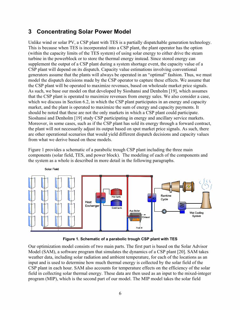
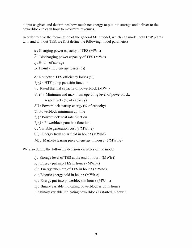
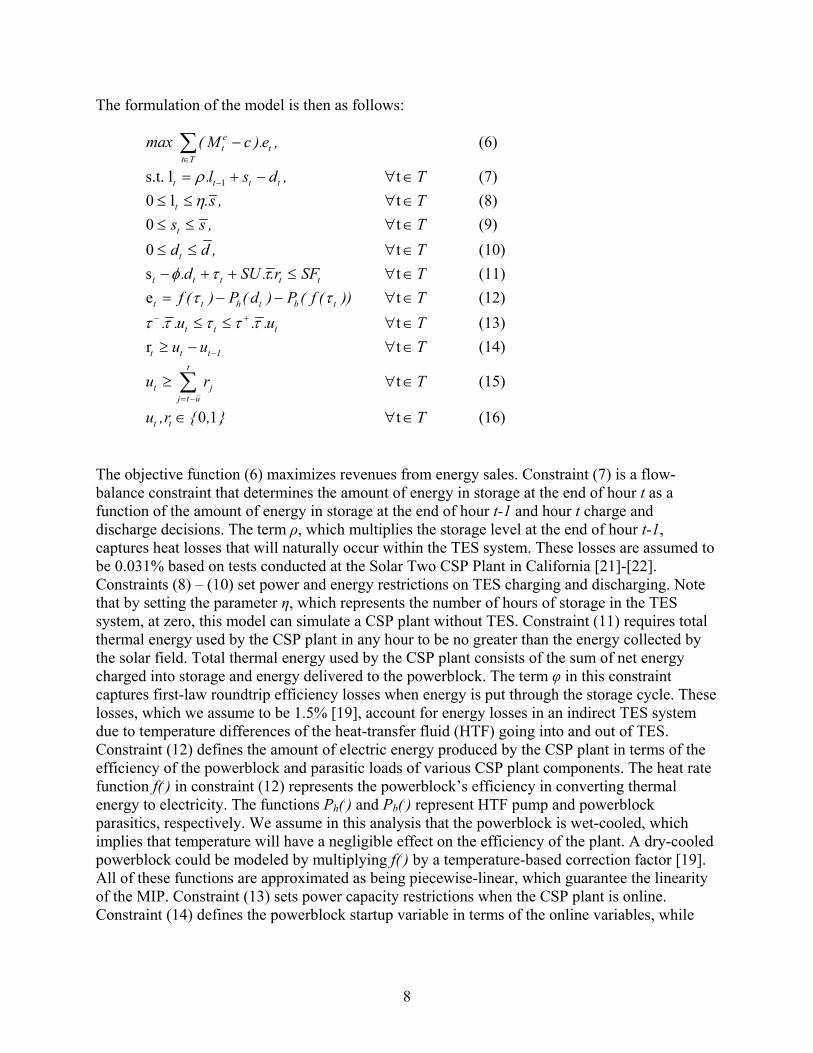
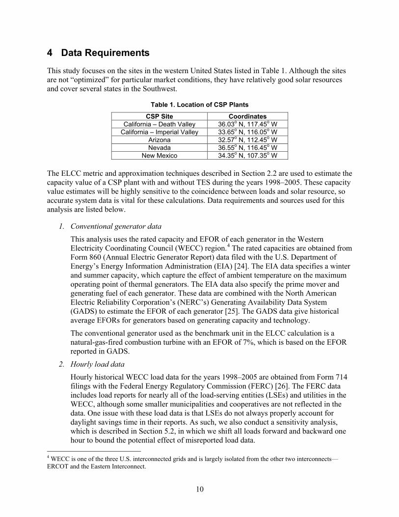
10
4 Data Requirements
This study focuses on the sites in the western United States listed in Table 1 Although the sites are not ldquooptimizedrdquo for particular market conditions they have relatively good solar resources and cover several states in the Southwest
Table 1 Location of CSP Plants
CSP Site Coordinates California ndash Death Valley 3603o N 11745o W
California ndash Imperial Valley 3365o N 11605o W Arizona 3257o N 11245o W Nevada 3655o N 11645o W
New Mexico 3435o N 10735o W
The ELCC metric and approximation techniques described in Section 22 are used to estimate the capacity value of a CSP plant with and without TES during the years 1998ndash2005 These capacity value estimates will be highly sensitive to the coincidence between loads and solar resource so accurate system data is vital for these calculations Data requirements and sources used for this analysis are listed below
1 Conventional generator data This analysis uses the rated capacity and EFOR of each generator in the Western Electricity Coordinating Council (WECC) region4
The conventional generator used as the benchmark unit in the ELCC calculation is a natural-gas-fired combustion turbine with an EFOR of 7 which is based on the EFOR reported in GADS
The rated capacities are obtained from Form 860 (Annual Electric Generator Report) data filed with the US Department of Energyrsquos Energy Information Administration (EIA) [24] The EIA data specifies a winter and summer capacity which capture the effect of ambient temperature on the maximum operating point of thermal generators The EIA data also specify the prime mover and generating fuel of each generator These data are combined with the North American Electric Reliability Corporationrsquos (NERCrsquos) Generating Availability Data System (GADS) to estimate the EFOR of each generator [25] The GADS data give historical average EFORs for generators based on generating capacity and technology
2 Hourly load data Hourly historical WECC load data for the years 1998ndash2005 are obtained from Form 714 filings with the Federal Energy Regulatory Commission (FERC) [26] The FERC data includes load reports for nearly all of the load-serving entities (LSEs) and utilities in the WECC although some smaller municipalities and cooperatives are not reflected in the data One issue with these load data is that LSEs do not always properly account for daylight savings time in their reports As such we also conduct a sensitivity analysis which is described in Section 52 in which we shift all loads forward and backward one hour to bound the potential effect of misreported load data
4 WECC is one of the three US interconnected grids and is largely isolated from the other two interconnectsmdashERCOT and the Eastern Interconnect
11
3 CSP generation profile In order to provide the most robust capacity value estimates multiple years of CSP generation data is needed Since no CSP plants are operating at the exact study locations5 we model the operation of a CSP plant using the optimization model developed by Sioshansi and Denholm [19] Data requirements for the model include hourly weather and historical energy price data for each location Hourly weather data are obtained from the National Solar Radiation Data Base6
5 The Nevada Solar One SEGS and Saguaro CSP plants are near the study locations however we opt to use the same modeled data for purposes of comparison
For the two CSP plants in California the California ISO market-clearing price of energy for the SP15 zone is used for the energy price in the optimization model (both of the plants studied are located in southern California which the SP15 zone covers) For CSP plants in Arizona Nevada and New Mexico load lambda data for Arizona Public Service (APS) Nevada Power (NP) and PNM (the largest utility in New Mexico) are used respectively The load lambda data are obtained from Form 714 filing with FERC [26] Since load lambda data for APS in the year 1999 is not available capacity values for the Arizona site are not calculated for this year
6 These data are available for download at httprredcnrelgovsolarold_datansrdb
12
5 Capacity Value of a Concentrating Solar Power Plant without Thermal Energy Storage
We begin by first computing capacity values of CSP plants without TES These calculations use CSP generation patterns which are optimized using the model described in equations (6) ndash (16) in the ELCC and capacity factor calculations Since we hold the size of the powerblock fixed the SM is the only size parameter that is adjusted in the plants that we simulate Figure 2 summarizes the average (over the eight years studied) annual capacity values obtained based on the ELCC method The capacity values are all normalized by the maximum net output of the CSP plant which is 120 MW-e7
Figure 2 shows that the SM has a direct impact on the capacity value of the CSP plant This is because a CSP plant with a small solar field will often operate below its rated capacity reducing its capacity value As the solar field size increases more thermal energy will be available during such hours increasing the capacity value On the other hand a large solar field will lead to greater capital costs and if the CSP plant does not have TES excess thermal energy that would exceed the powerblock rating will be wasted [19] Sioshansi and Denholm [19] provide estimates of the amount of solar thermal energy wasted by a CSP plant without TES as a function of solar field size While the range of SMs shown is 10ndash30 the typical range of SMs for plants with storage is closer to 13ndash15 The optimal solar field size for a CSP plant without TES will depend on the relative capital cost of the components and the incremental value of the added energy and capacity value If the CSP plant is coupled with TES on the other hand excess energy that would exceed the powerblock rating could be stored and used in later hours This can make investments in larger solar fields reasonable and also increase the capacity and energy value of the plant Selecting an appropriate or optimal solar field size requires an in-depth economic analysis
7 The same normalizing is done for all of the capacity value estimates in this report
13
10 12 14 16 18 20 22 24 26 28 3010
20
30
40
50
60
70
80
90
100
SM
Nor
mal
ized
Cap
acity
Val
ue (
)
Arizona LocationImperial Valley LocationDeath Valley LocationNevada LocationNew Mexico Location
Figure 2 Average annual capacity value of a CSP plant with no TES in different locations
Figure 2 also shows that the rank ordering of the locations in terms of capacity value can vary as a function of solar field size This is because adjusting the solar field size will change the operation of the CSP plants In some cases increasing the SM will allow the powerblock to start up during a high-LOLP hour when it would otherwise not be able to with a smaller solar field due to minimum-load constraints on the powerblock For instance with an SM of 14 or less the Death Valley location has the highest capacity value whereas the Arizona location has the highest capacity value with an SM of 15 or greater
Figure 2 represents average annual capacity values over the eight years of study Capacity values can however vary significantly from year to year This is also true for conventional generators since a forced outage during a high-LOLP hour would yield a low capacity value in the year in which it occurs Figure 3 shows capacity values for a CSP plant at the New Mexico location over the eight individual years The differences in annual capacity values reinforce the fact that several years of generation data are required to provide a robust capacity value estimate for CSP
14
10 12 14 16 18 20 22 24 26 28 3010
20
30
40
50
60
70
80
90
100
SM
Nor
mal
ized
Cap
acity
Val
ue (
)
20032000199920052002199820012004
Figure 3 Annual capacity value of a CSP plant with no TES at the New Mexico location
Figure 3 shows that with an SM of 10 the capacity value of the CSP plant in the year 2000 is more than four times greater than that in the year 2004 In order to better understand the reason behind this the operations of the CSP plant during the highest-LOLP hours in those two years need to be compared In the year 2000 the highest-LOLP hours occur on August 1 Figure 4 shows the hourly output of the CSP plant and LOLPs on this day and shows that the plant has an average output of about 85 MW-e during the highest-LOLP hours Since the output of the CSP is correlated with the LOLPs a high capacity value for the plant can be expected Figure 5 shows the amount of thermal solar energy collected by the solar field which reflects the amount of solar irradiance and load data As can be seen in Figure 5 load data is strongly correlated with solar energy This correlation is reasonable during a summer day due to the fact that summer loads are driven by cooling needs which will be correlated with solar availability
15
2 4 6 8 10 12 14 16 18 20 22 240
10
20
30
40
50
60
70
80
90
100
110
Ene
rgy
(MW
-e)
Hour2 4 6 8 10 12 14 16 18 20 22 24
0
01
02
03
04
05
LOLP
LOLPCSP Generation
Figure 4 Hourly LOLPs and dispatch of a CSP plant with no TES at the New Mexico location with
an SM of 10 on August 1 2000
1 2 3 4 5 6 7 8 9 10 11 12 13 14 15 16 17 18 19 20 21 22 23 240
100
200
300
400
500
600
700
800
900
1000
Hour
Dire
ct N
orm
al Ir
radi
ance
(Wm
2 )
1 2 3 4 5 6 7 8 9 10 11 12 13 14 15 16 17 18 19 20 21 22 23 2460
70
80
90
100
110
120
Load
(GW
)
LoadSolar Radiation
Figure 5 Hourly loads and solar radiation at the New Mexico location on August 1 2000
Figure 6 shows the operations of the CSP plant on August 10 2004 which is the day with the highest LOLPs of that year The figure shows that CSP generation is not correlated with LOLPs in this case Hence the capacity value of the CSP plant is relatively lower in 2004 compared to 2000 Figure 7 shows the amount of thermal solar energy collected by the solar field and load
16
data for the day Unlike the case shown in Figure 5 electricity demand is less correlated with solar energy which causes lower capacity value in 2004
1 2 3 4 5 6 7 8 9 10 11 12 13 14 15 16 17 18 19 20 21 22 23 24
0
10
20
30
40
50
60
70
80
90
100
Hour
Ene
rgy
(MW
h-e)
1 2 3 4 5 6 7 8 9 10 11 12 13 14 15 16 17 18 19 20 21 22 23 240
01
02
03
04
05
LOLP
LOLPCSP Generation
Figure 6 Hourly LOLPs and dispatch of a CSP plan with no TES at the New Mexico location with
an SM of 10 on August 10 2004
1 2 3 4 5 6 7 8 9 10 11 12 13 14 15 16 17 18 19 20 21 22 23 240
100
200
300
400
500
600
700
800
900
1000
Hour
Dire
ct N
orm
al Ir
radi
ance
(Wm
2 )
1 2 3 4 5 6 7 8 9 10 11 12 13 14 15 16 17 18 19 20 21 22 23 2460
70
80
90
100
110
120
Load
(GW
)
LoadSolar Radiation
Figure 7 Hourly loads and solar radiation at the New Mexico location on August 10 2004
Due to computational complexity and data requirements of the ELCC method using an approximation method to estimate the capacity value of a CSP plant may be preferred Doing so
17
can significantly reduce the computational time of the estimation but may affect the accuracy of the results We compare the ELCC calculations to three approximation techniques that are based on the capacity factor of the plant The first two use the highest-load and highest-LOLP hours of the year whereas the third uses the highest-load hours but weighs the capacity factors by the hourly LOLPs These three techniques are referred to as the ldquoTop Loadsrdquo ldquoTop LOLPrdquo and ldquoTop Weightedrdquo techniques hereafter Figures 8 through 10 show the average annual capacity values of a CSP plant at the Imperial Valley location based on the three approximation techniques The figures show the capacity value estimates when considering the top 10 top 100 and top 10 of hours of each year respectively
10 12 14 16 18 20 22 24 26 28 3010
20
30
40
50
60
70
80
90
100
SM
Nor
mal
ized
Cap
acity
Val
ue (
)
ELCCTop WeightedTop LOLPTop Load
Figure 8 Annual average capacity value of a CSP plant with no TES at the Imperial Valley location
using the ELCC metric and approximation techniques that select the top 10 hours
18
10 12 14 16 18 20 22 24 26 28 3010
20
30
40
50
60
70
80
90
100
SM
Nor
mal
ized
Cap
acity
Val
ue (
)
ELCCTop WeightedTop LOLPTop Load
Figure 9 Annual average capacity value of a CSP plant with no TES at the Imperial Valley location
using the ELCC metric and approximation techniques that select the top 100 hours
10 12 14 16 18 20 22 24 26 28 3010
20
30
40
50
60
70
80
90
100
SM
Nor
mal
ized
Cap
acity
Val
ue (
)
ELCCTop WeightedTop LOLPTop Load
Figure 10 Annual average capacity value of a CSP plant with no TES at the Imperial Valley
location using the ELCC metric and approximation techniques that select the top 10 of hours
19
Comparing Figures 8 through 10 shows that using an approximation method that considers only the top 10 hours of each year yields a capacity value estimate that is closest to the ELCC metric The figures also show that the ldquoTop Weightedrdquo approximation tends to have greater accuracy Similar results are obtained for the other sites This is demonstrated in Figures 11 through 14 which compare the three approximation techniques when considering only the top 10 hours of each year to the ELCC calculation for the other locations
10 12 14 16 18 20 22 24 26 28 3010
20
30
40
50
60
70
80
90
100
SM
Nor
mal
ized
Cap
acity
Val
ue (
)
ELCCTop WeightedTop LOLPTop Load
Figure 11 Annual average capacity value of a CSP plant with no TES at the New Mexico location
using the ELCC metric and approximation techniques that select the top 10 hours
20
10 12 14 16 18 20 22 24 26 28 3030
40
50
60
70
80
90
100
SM
Nor
mal
ized
Cap
acity
Val
ue (
)
ELCCTop WeightedTop LOLPTop Load
Figure 12 Annual average capacity value of a CSP plant with no TES at the Death Valley location
using the ELCC metric and approximation techniques that select the top 10 hours
10 12 14 16 18 20 22 24 26 28 3010
20
30
40
50
60
70
80
90
100
SM
Nor
mal
ized
Cap
acity
Val
ue (
)
ELCCTop WeightedTop LOLPTop Load
Figure 13 Annual average capacity value of a CSP plant with no TES at the Nevada location using
the ELCC metric and approximation techniques that select the top 10 hours
21
10 12 14 16 18 20 22 24 26 28 3010
20
30
40
50
60
70
80
90
100
SM
Nor
mal
ized
Cap
acity
Val
ue (
)
ELCCTop LOLPTop LoadTop Weighted
Figure 14 Annual average capacity value of a CSP plant with no TES at the Arizona location using
the ELCC metric and approximation techniques that select the top 10 hours
51 Effect of Expected Forced Outage Rates on Concentrating Solar Power Capacity Value
Our analysis thus far is based on modeling a system in which the conventional generator set varies from year to year This is because we only model conventional generators that were in operation in each year and this generator set changes from year to year as a result of generator construction and retirements Moreover the EFORs that are reported in the NERC GADS database are annual values which will also vary from year to year depending on how many outages actually occurred We use these annual EFORs to capture the fact that outage rates can vary from year to year These differences in the conventional generator mix and EFORs can contribute to the differences in the annual capacity values of the CSP plants which are shown in Figure 3 Figure 15 compares the average annual ELCC of a CSP plant at the Imperial Valley location in cases in which these parameters vary to a case in which these parameters are held constant In the cases in which the parameters are held constant we use the conventional generator mix that was installed in 2005 and EFORs that are averaged over the eight study years Figure 15 shows that the ELCC values are nearly identical with very little differences for smaller-sized CSP plants The other locations have very similar results As such we can conclude that variations in the mix and reliability of other generators will have a negligible impact on the capacity value of a CSP plant
22
10 12 14 16 18 20 22 24 26 28 3010
20
30
40
50
60
70
80
90
100
SM
Nor
mal
ized
Cap
acity
Val
ue (
)
Different Gen Set and EFORSame Gen Set and EFOR
Figure 15 Average annual capacity value of a CSP plant with no TES at the Imperial Valley location based on ELCC metric with constant and varying conventional generator characteristics
52 Effect of Load Errors on Concentrating Solar Power Capacity Value As noted before another issue with our capacity value estimates is that some utilities do not properly account for daylight savings time in reporting their hourly loads in FERC Form 714 filings As such it is possible that the simulated output of the CSP plant could be offset from the system loads and LOLPs Since the capacity value of CSP is highly dependent on the correlation between solar resource availability and load this potential mismatch in the data can lead to different capacity values than what we have estimated thus far In order to bound the effect of misreported load data we conduct the same ELCC calculations but shift the loads forward and backward one hour Figure 16 shows average annual ELCC values for a CSP plant at the Imperial Valley location when the system loads are shifted in this way and it compares them to the base case in which the reported loads are used without shifting The figure shows that this shifting in the loads can reduce the estimated capacity value of a CSP plant by up to 5 the other locations have similar results The ELCC is reduced regardless of whether the load is shifted forward or backward which suggests that most of the loads reported in the Form 714 data are correct This is because solar resource and CSP generation will have some correlation with system loads and this correlation is maximized when the loads are not shifted
23
10 12 14 16 18 20 22 24 26 28 3010
20
30
40
50
60
70
80
90
100
SM
Nor
mal
ized
Cap
acity
Val
ue (
)
Base CaseShift Load One Hour ForwardShift Load One Hour Backward
Figure 16 Average annual capacity value of a CSP plant with no TES at the Imperial Valley location based on ELCC metric with loads shifted
53 Effect of Sub-Hourly Variability on Concentrating Solar Power Capacity
Value Our analysis thus far is based on using hourly solar data and modeled CSP generation to calculate ELCCs and capacity factors Solar radiation can have noticeable sub-hourly variation due to passing cloud cover Sub-hourly variation may impact the capacity value and integration costs of many renewable resources such as wind and solar PV CSP may not suffer from this issue as much however since the HTF of a CSP plant will have some thermal inertia which can maintain output during a brief reduction in solar radiation Indeed a CSP plant with direct TES will not suffer from short-term transients at all since the powerblock is fed by the TES system and not directly from the solar field
In order to determine the effect of sub-hourly variability on the capacity value of CSP we compare our ELCC calculations when CSP output is modeled using one-minute and hourly data We use one-minute solar data for a CSP plant located around the Nevada One site in Boulder City Nevada The coordinates of the modeled location are 3580o N 11497o W We use one-minute weather data from the year 2007 and compare a case in which the CSP plant is modeled using the one-minute data to a case in which hourly averages of the one-minute data are used instead SAM and the CSP dispatch model are both adapted to model one-minute operations by appropriate scaling of the model variables and parameters The same hourly conventional generator and load data are used in both cases thus any differences in the ELCC estimates are solely due to the one-minute weather data as opposed to hourly averages Since the loads are
24
assumed constant during each hour these ELCC estimates will not capture sub-hourly load variations and potential correlation between these and solar radiation patterns
Figure 17 shows the ELCC estimates for the CSP plant as a function of the solar field size using the one-minute and hourly average data The results show that the hourly average data will provide a close approximation of the ELCC if one-minute data is used The maximum difference in the ELCC between the one-minute and hourly average data is 58 For most plant configurations the hourly average data tends to overestimate the ELCC This is because with one-minute data subhourly variations in solar radiation can keep the powerblock from running above its minimum operating point These variations are not fully captured when the one-minute data is averaged The differences in the estimated ELCCs are maximized for plants with an SM between 24 and 28 This is because plants with this configuration have more time periods in which solar radiation variability can prevent the powerblock from starting up which is not captured without hourly data Despite these issues the small difference in the ELCC values suggest that hourly data can provide relatively good capacity value estimates if sub-hourly data is not available or too computationally intensive to work with
10 12 14 16 18 20 22 24 26 28 3010
20
30
40
50
60
70
80
90
100
SM
Nor
mal
ized
Cap
acity
Val
ue (
)
Hourly Solar DataOne-Minute Solar Data
Figure 17 Capacity value of a CSP plant with no TES at the Boulder City Nevada location based
on ELCC metric while using hourly and one-minute interval solar data
25
6 Capacity Value of a Concentrating Solar Power Plant with Thermal Energy Storage
A major benefit of coupling CSP with TES is that TES will make the CSP plant more dispatchable This is because TES allows the CSP plant to store excess energy collected by the solar field when it is not needed and discharge that energy later when solar resources are lower Our results in Section 5 clearly show that the ability of a CSP plant to generate electricity in critical peak hours with high loads or LOLPs has a significant impact on capacity value Therefore adding TES to a CSP plant can increase its capacity value by allowing it to generate electricity during critical periods when solar resources are not available As suggested earlier adding TES to a CSP plant can also make a higher SM more economic since excess thermal solar energy collected by the solar field will not be wasted and can be stored and later used
Estimating the capacity value of a CSP plant is more complicated when it has a TES system This is because a proper capacity value estimate must not only account for how much energy the plant generates each hour but also how much energy it could produce using energy in storage One must account for energy in storage because if a system shortage event occurs the CSP plant would in principle use energy in storage to help support the system Modeling energy in storage is difficult because of the energy-limited nature of energy storage Namely if energy in TES is used in hour t then it cannot be used in any hour s gt t A previous capacity value estimation technique for energy storage technologies was developed by Tuohy and OrsquoMalley [23] and applied to pumped hydroelectric storage (PHS) Their technique uses operational data to determine the maximum potential output of the PHS device in each hour if the energy in storage is discharged at maximum capacity (based on the available energy in storage) The capacity value of the PHS device is then estimated from the maximum potential output data using a capacity-factor-based approximation technique
We apply a similar approach to estimate the capacity value of the CSP plant with TES As in the case without TES we assume that the operation of the CSP plant and TES is optimized to maximize the revenues that the CSP plant receives Once the operation of the CSP plant is established we can determine the maximum potential output of the CSP plant by first computing the maximum amount of thermal energy that can be delivered from the solar field and TES to the power block in each hour as
1min min (1 ) (17)t t t tSF d l SU umicroτ τ τ φ ρ τ+minus= + minus minus
Equation (17) defines the maximum thermal energy that can be delivered to the powerblock in each hour ( t
microτ ) as the minimum of the powerblockrsquos rated capacity ( +τ τ ) and the sum of thermal energy collected by the solar field and the amount of energy available in TES ( 1min minus+t tSF d lφ ρ ) Equation (17) assumes that if the powerblock is offline it can be committed within the hour in case of a system shortage event [27] We can also define how much of the t
microτ MWh-t is taken from TES as
(18)t t td SFmicro microτ= minus
26
Finally the maximum potential output of the CSP plant etmicro is given by
e ( ) ( ) ( ( )) (19)t t h t b tf P d P fmicro micro micro microτ τ= minus minus
Once we determine the maximum potential output we estimate the capacity value using the top weighted approximation technique considering the 10 highest-load hours of each year since our results in Section 5 show this to be the most accurate approximation
We model the operations of the CSP plant under two different market settings The first is an energy-only market in which the CSP plant only receives payments for the electricity that it supplies to the market The operation of the CSP plant in the energy-only market setting is optimized using the model given in Section 3 and is represented by objective function (6) and constraints (7) through (16) The other market setting that we examine is one in which the CSP plant can receive energy and capacity payments In this case the optimization model must be changed to co-optimize the sum of energy and capacity payments Further details of the capacity payment model are given in Section 62
61 Capacity Value of a Concentrating Solar Power Plant with Thermal Energy Storage in an Energy-Only Market
Figures 18 through 22 summarize the average annual capacity value of CSP plants at the different locations that we study The figures show that the capacity values are typically increasing with the SM and the hours of TES in the CSP plant although this relationship is not perfectly monotonic At all of the locations adding some TES increases the capacity value of the plant above the no-TES case For instance a CSP plant at the New Mexico location with an SM of 15 and no TES has a capacity value of about 78 MW-e Adding one hour of TES to this plant addresses many of the days on which solar and load are not well correlated and increases its capacity value by 47 to 115 MW-e
27
0 2 4 6 8 10 1260
65
70
75
80
85
90
95
100
Hours of TES
Nor
mal
ized
Cap
acity
Val
ue (
)
SM 27
SM 23SM 19
SM 15
Figure 18 Average annual capacity value of a CSP plant with TES at the Imperial Valley location
under an energy-only market setting
0 2 4 6 8 10 1260
65
70
75
80
85
90
95
100
Hours of TES
Nor
mal
ized
Cap
acity
Val
ue (
)
SM 27
SM 23SM 19
SM 15
Figure 19 Average annual capacity value of a CSP plant with TES at the New Mexico location
under an energy-only market setting
28
0 2 4 6 8 10 1260
65
70
75
80
85
90
95
100
Hours of TES
Nor
mal
ized
Cap
acity
Val
ue (
)
SM 27
SM 23SM 19
SM 15
Figure 20 Average annual capacity value of a CSP plant with TES at the Death Valley location
under an energy-only market setting
0 2 4 6 8 10 1260
65
70
75
80
85
90
95
100
Hours of TES
Nor
mal
ized
Cap
acity
Val
ue (
)
SM 27
SM 23SM 19
SM 15
Figure 21 Average annual capacity value of a CSP plant with TES at the Nevada location under an
energy-only market setting
29
0 2 4 6 8 10 1260
65
70
75
80
85
90
95
100
Hours of TES
Nor
mal
ized
Cap
acity
Val
ue (
)
SM 27
SM 23SM 19
SM 15
Figure 22 Average annual capacity value of a CSP plant with TES at the Arizona location under an
energy-only market setting
In some cases however adding an incremental hour of TES or increasing the solar field size may cause a slight reduction in the capacity value of a plant This is because different CSP plant configurations will yield different operational decisions and in some cases a larger CSP plant may have less energy in TES during a high-LOLP hour For example a CSP plant at the Nevada location with four hours of TES and an SM of 22 has a capacity value of 117 MW-e in 1999 The same CSP plant with an SM of 27 would have a lower capacity value of only 95 MW-e in 1999 This difference in the capacity value is due to less energy being in the TES of the larger CSP plant on July 12 which is the day with 5 of the 10 highest hourly LOLPs of the year The larger CSP plant has less energy in storage because the larger solar field provided sufficient energy to operate the powerblock above its minimum operating point in the afternoon of the previous day The smaller solar field of the CSP plant with an SM of 22 could not meet this minimum-load constraint and as such the output of the solar field was stored Thus the CSP plant with an SM of 22 can on average generate up to 74 MW-e during the five highest-LOLP hours on July 12 The larger CSP plant with an SM of 27 can only generate up to an average of 54 MW-e during these hours Figure 23 shows the amount of energy in storage and energy collected by the solar field in each hour on July 12 for these two CSP plant configurations It is important to note that due to weather patterns on this particular day the solar field only collects solar energy during hour 18mdashthe output of the field is zero in the remaining hours
30
Figure 23 LOLP energy from solar field and energy in storage for a CSP plant at the Nevada location with four hours of TES and different SM values on July 12 1999
Adding TES can also in some cases reduce the capacity value of the CSP plant although this is less typical For example a CSP plant at the Death Valley location with an SM of 27 and one hour of TES has a capacity value of 79 MW-e in 1999 Increasing TES by one hour for the same CSP plant reduces its capacity value to 75 MW-e The reduction in capacity value stems from the fact that energy prices are not necessarily correlated with hours with highest LOLPs as suggested by Figure 24 which is a scatter plot of California ISO energy prices and LOLPs in the year 1999 The operation of both of the CSP plants on July 12 which is the day on which the highest LOLPs of the year occur is shown in Figure 25
31
Figure 24 LOLP versus energy price for the Death Valley location in year 1999
Note The x-axis used to represent LOLPs has a logarithmic scale
Figure 25 LOLP energy from solar field and energy in storage for a CSP plant at the Death Valley
location with an SM of 27 and different TES sizes on July 12 1999
32
Figure 25 shows that in hour 16 during which the LOLP is the highest the larger CSP plant has less energy in storage compared to the smaller CSP plant This reduces the capacity value of the larger CSP plant The reason behind these operations is that in hours 12 through 15 of the day the larger CSP plant will use energy in TES to generate electricity since energy prices are higher in these hours than in hours during which the highest LOLPs occur The smaller CSP cannot do so since its smaller TES system does not have sufficient energy in storage to operate above its minimum generation point during these hours These operational differences leave the smaller CSP plant with more energy in TES during hour 16 which yield the higher capacity value
62 Capacity Value of a Concentrating Solar Power Plant with Thermal Energy Storage in a Capacity Market
In Section 61 we estimate the capacity value of a CSP plant with TES in an energy-only market The results there suggest that adding TES to a CSP plant will tend to increase the capacity value of the plant although this relationship is not monotonic This is because energy prices and LOLPs will not always be perfectly correlated and there can be high-LOLP hours that have lower energy prices than other hours with lower LOLPs An example of this is demonstrated in Figure 25 An alternative market design that could help reduce the impact of such price and LOLP patterns is an energy and capacity market Under such a market design the CSP plant receives both payments for electricity that it generates as well as the capacity that it provides the system Many electricity markets have moved toward adopting capacity markets Even in systems that do not have an explicit capacity market such as the APS NP and PNM service territories a model that maximizes the sum of energy and capacity payments may be more appropriate This is because such integrated utilities would likely operate a CSP plant to minimize its overall energy supply costsmdashwhich would be akin to our energy revenue maximization However such utilities would also likely adjust the operation of their plants to have more energy available in TES during anticipated system shortage events
The introduction of a capacity market tends to increase the capacity value of a CSP plant since capacity payments typically have performance requirements that are related to the capacity value of a generator Most capacity markets impose financial penalties on generators that do not meet the performance requirements Although the specific performance requirements differ from market to market they are typically related to how much firm capacity a generator has available during system shortage events Our capacity market model is based on the forward capacity market (FCM) used by ISO New England although the modeling framework is sufficiently general that it can be adapted to model other markets as well
621 Capacity Market Procedures The objective of a capacity market is to encourage enough generating capacity to enter the system so that reliability requirements are met This objective is met by a forward capacity auction (FCA)8
8 These auctions are held three years in advance for ISO New Englandrsquos FCM
Resources that participate and are selected in the FCA are eligible to receive capacity payments throughout the capacity commitment period based on their capacity commitment obligations Capacity payments are subject to certain performance requirements however Performance requirements are set so that the capacity resources contribute to system reliability during hours in which shortage events could occur The definition of shortage events will differ between capacity markets Some markets such as the FCM define shortage events as
33
periods during which reserves (spinning and non-spinning reserves) fall below certain levels This definition does not necessarily imply that supply is less than demand during the shortage event hours For instance if the reserve level falls to 1 generating capacity will still be greater than demand but due to low reserve levels the probability of having a capacity deficiency is high Based on this definition there is a one-to-one relationship between shortage event hours and the hourly LOLPs In this study the 10 hours of each year with the highest LOLPs are defined as shortage event hours
A generator that fails to provide its contracted capacity during a shortage event hour will incur financial penalties The FCM sets penalties based on the cost of replacement capacity We assume that the capacity market uses the cost of a natural-gas-fired combustion turbine which we assume to be $671kW in 2008 dollars to set the penalties This cost is then translated into an annualized cost of $7381kW-year using an 11 capital charge rate We assume that the capacity market imposes a penalty that is equal to half of this annualized cost which is reflective of the penalties imposed in the FCM We use consumer price index data to deflate the cost of the combustion turbine to previous-year dollars
622 Optimization Model In order to determine the operations of a CSP plant in an energy- and capacity-market setting our model must be adjusted to maximize the sum of energy and capacity payments and net of any capacity penalties We follow a similar approach to that used in Section 61 and add variables to our optimization model that determine the maximum potential generation from the CSP plant in each hour (based on energy in TES and collected by the solar field) The difference between the firm capacity sold and this maximum potential generation is the shortfall from the capacity commitment and these shortfalls are penalized in the objective function to reflect capacity penalties In order to give the formulation of the model we define the following parameters
Market clearing price of capacity ($MW-year) Penalty factor for unserved capacity requirements
Set of hours during which shortage events occur
cMPFH
We also define the following variables
Firm capacity sold
e Maximum potential net electric energy (MWh-e) produced by powerblock in each hoursold
t
Cmicro
Maximum potential thermal energy taken out of storage (MWh-t) in each hour
Maximum potential total thermal energy (MWh-t) fed to powerblock in each hour
Shortfall from capacity commit
t
tshortt
d
C
micro
microτ
ment in each hour
The formulation of the model is then given by
max short
e c c tt t sold
t T t H sold
C( M c )e M C ( M PF )
Cisin isin
minus + minussum sum (20)
34
st (7)-(16) e short
t sold tC C microge minus t Tforall isin (21)
1 t td lmicro ρ minusle t Tforall isin (22) t t t td SU r SFmicro microφ τ τminus + + le t Tforall isin (23)
e t t h t b tf ( ) P ( d ) P ( f ( ))micro micro micro microτ τ= minus minus t Tforall isin (24)
t t t u umicroτ τ τ τ τminus +le le t Tforall isin (25)
Objective function (20) maximizes the sum of net energy and capacity revenues The last term in the objective function corresponds to penalties associated with shortfalls from capacity commitments Constraints (7) through (16) which are from the original energy-only model are included since the same underlying constraints on the operation of the CSP plant apply Constraint (21) defines the hourly capacity commitment shortfall as the difference between firm capacity sold and the maximum potential net electrical generation of the CSP plant Constraint (22) restricts the potential thermal energy taken out of storage (MWh-t) in each hour based on the ending storage level of the previous hour Constraint (23) limits the total amount of potential thermal energy used in the CSP plant to not be greater than the energy collected by the solar field Constraint (24) defines the maximum potential output of the CSP plant in each hour Finally constraint (25) imposes restrictions on potential capacity of the CSP plant when the powerblock is online
Because the penalty term in the objective function is non-linear in the variables we solve this model by fixing the value of Csold and solving the model iteratively until finding a maximum For the cases that we consider selling 120 MW-e of capacity (the maximum net output of the CSP plant) maximizes CSP revenues
623 Results The model given by objective function (20) and constraints (7) through (16) and (21) through (25) is used to determine the optimized operation of the CSP plant in each hour We then apply the same capacity-factor-based approximation technique used in Section 61 to estimate the capacity value of the plant Figures 26 through 30 summarize the average annual capacity value of the CSP plants at the different locations
35
0 2 4 6 8 10 1260
65
70
75
80
85
90
95
100
Hours of TES
Nor
mal
ized
Cap
acity
Val
ue (
)
SM 27
SM 23SM 19
SM 15
Figure 26 Average annual capacity value of a CSP plant with TES at the Imperial Valley location
under an energy and capacity market setting
0 2 4 6 8 10 1260
65
70
75
80
85
90
95
100
Hours of TES
Nor
mal
ized
Cap
acity
Val
ue (
)
SM 27
SM 23SM 19
SM 15
Figure 27 Average annual capacity value of a CSP plant with TES at the New Mexico location
under an energy and capacity market setting
36
0 2 4 6 8 10 1260
65
70
75
80
85
90
95
100
Hours of TES
Nor
mal
ized
Cap
acity
Val
ue (
)
SM 27
SM 23SM 19
SM 15
Figure 28 Average annual capacity value of a CSP plant with TES at the Death Valley location
under an energy and capacity market setting
0 2 4 6 8 10 1260
65
70
75
80
85
90
95
100
Hours of TES
Nor
mal
ized
Cap
acity
Val
ue (
)
SM 27
SM 23SM 19
SM 15
Figure 29 Average annual capacity value of a CSP plant with TES at the Nevada location under an
energy and capacity market setting9
9 The unusual result for Nevada (compared to the other locations) is due to a day in 1999 where an SM of less than 27 was insufficient to meet the minimum generation requirement during one 3-hour period of high LOLP This demonstrates the need to examine performance over a large period of time to examine the impact of variability on resource adequacy
37
0 2 4 6 8 10 1260
65
70
75
80
85
90
95
100
Hours of TES
Nor
mal
ized
Cap
acity
Val
ue (
)
SM 27
SM 23SM 19
SM 15
Figure 30 Average annual capacity value of a CSP plant with TES at the Arizona location under an
energy and capacity market setting
Figures 26 through 30 show the benefits of implementing a capacity payment scheme as opposed to an energy-only market Adding capacity payments tends to slightly increase the capacity value of the CSP plant Moreover the capacity value is more monotonic in the size of the plant There are still however some cases in which increasing the size of a CSP plant can result in a slight reduction in the capacity value Even when the capacity payment is added there may still be high-LOLP hours in which the value of energy (when accounting for the energy price and capacity penalty) is lower than other hours with lower LOLPs However these cases are rare and their magnitude (in terms of capacity value reductions) is relatively small
More broadly contrasting these results with the energy-only market design and Figure 23 in particular demonstrates the benefit of capacity payments (or co-optimizing the energy and capacity value of a CSP plant) in improving the system benefits of CSP Figure 23 shows that the larger CSP plant has a lower capacity value because of poor correlation between energy prices and LOLPs and the lack of solar resource during high-LOLP hours If a CSP plant can anticipate potential high-LOLP periods or shortage events the total value of the plant to the system can be drastically increased by slightly adjusting plant operations
38
7 Conclusions
This study estimates the capacity value of a CSP plant at a variety of locations within the WECC while accounting for rational dispatch behavior of a CSP operator This is done by optimizing the operation of the CSP plant and by using standard reliability-based capacity value estimation techniques Although the ELCC metric is the most accurate estimation technique we show that capacity-factor-based approximation methods can closely estimate the ELCC value
When introducing TES the capacity value of the CSP plant is more difficult to estimate since one must account for energy in storage We apply the capacity-factor-based technique used by Tuohy and OrsquoMalley [23] under two different market settings an energy-only market and an energy and capacity market Our results show that adding TES to a CSP plant can increase its capacity value significantly at all of the locations Adding a single hour of TES significantly increases the capacity value above the no-TES case in most cases to above 90 Although additional hours of TES increase the capacity value of the plant their marginal benefit is less than the first hour of TES Nevertheless Sioshansi and Denholm [19] show that a greater number of hours of TES can have incremental energy and ancillary service benefits Since energy prices LOLPs and solar resource will not be perfectly correlated the use of capacity payments (or co-optimization of energy and capacity value) can significantly increase the value of a CSP plant to the power system compared to an energy-only market
The capacity value estimates we provide examine a single CSP plant which will have a marginal effect on the rest of the system Clearly changes in the generation mix or load patterns could affect the capacity value of a CSP plant Adding more CSP (or PV) plants especially if they are concentrated at similar locations in the system can reduce the marginal capacity value of additional CSP capacity Adding TES to a CSP plant can alleviate this reduction in the marginal capacity value however since it gives the CSP plant additional flexibility in dispatching its generation
39
References
[1] Soumlder L Amelin M ldquoA Review of Different Methodologies Used for Calculation of Wind Power Capacity Creditrdquo Proceedings of the IEEE Power Engineering Society General Meeting 2008 Pittsburgh PA 2008
[2] Pudaruth GR Li F Capacity Credit Evaluation A Literature Review Third International Conference on Electric Utility Deregulation and Restructuring and Power Technologies DRPT 2008 Nanjing China pp 2719ndash2724
[3] Milligan M Porter K ldquoDetermining the Capacity Value of Wind An Updated Survey of Methods and Implementationrdquo WindPower 2008 June 2008 Houston Texas
[4] Billinton R Allan R Reliability Evaluation of Power Systems 2nd edition New York Plenum Press 1984
[5] Kahn EP ldquoEffective Load Carrying Capability of Wind Generation Initial Results with Public Datardquo The Electricity Journal Vol 17 Iss 10 December 2004 pp 85ndash95
[6] Amelin M ldquoComparison of Capacity Credit Calculation Methods for Conventional Power Plants and Wind Powerrdquo IEEE Trans Power Syst Vol 24 No 2 May 2009
[7] Ensslin C Milligan M Holttinen H OrsquoMalley M Keane A ldquoCurrent Methods to Calculate Capacity Credit of Wind Power IEA collaborationrdquo Proceedings 2008 IEEE Power amp Energy Society General Meeting 2008 p 3
[8] Milligan M Parsons B ldquoA Comparison and Case Study of Capacity Credit Algorithms for Intermittent Generatorsrdquo Proceedings Solar rsquo97 April 27ndash30 1997 Washington DC NRELCP-440-22591 Golden CO National Renewable Energy Laboratory March 1997
[9] Keane A Milligan M DAnnunzio C Dent CJ Dragoon K Hasche B Holttinen H Samaan N Sumloder L OMalley M ldquoCapacity Value of Wind Powerrdquo IEEE Trans Power Syst forthcoming
[10] DrsquoAnnunzio C Santoso S ldquoNoniterative Method to Approximate the Effective Load Carrying Capability of a Wind Plantrdquo IEEE Trans Energy Conv Vol 23 No 2 June 2008 pp 544ndash550
[11] Martin B Diesendorf M ldquoCalculating the Capacity Credit of Wind Powerrdquo Proceedings 4th Biennial Conference University of Queensland August 1980 Brisbane Queensland Australia pp 36ndash42
[12] Garver LL ldquoEffective Load Carrying Capability of Generating Unitsrdquo IEEE Trans on PAS Vol PAS-85 August 1966 pp 910ndash919
[13] Hoff T Perez R Ross JP Taylor M ldquoPhotovoltaic Capacity Valuation Methodsrdquo SEPA REPORT 02-08 Washington DC Solar Electric Power Association 2008
40
[14] Bernow S Biewald B Singh D ldquoModelling Renewable Electric Resources A Case Study of Wind Reliabilityrdquo Presented at the NARUC-DOE National Conference on Renewable Energy Savannah GA October 1993
[15] El-Sayed M ldquoSubstitution Potential of Wind Energy in Egyptrdquo Energy Policy Vol 30 2002 pp 681ndash687
[16] Milligan M Parsons B ldquoA Comparison and Case Study of Capacity Credit Algorithms for Wind Power Plantsrdquo Wind Energy Vol 23 Iss 3 1999 pp 159ndash166
[17] Milligan M Porter K ldquoThe Capacity Value of Wind in the United States Methods and Implementationrdquo The Electricity Journal Vol 19 Iss 2 March 2006
[18] Milligan M Modeling Utility-scale Wind Power Plants Part 2 Capacity Credit NRELTP-500-27514 Golden CO National Renewable Energy Laboratory June 2000
[19] Sioshansi R Denholm P ldquoThe Value of Concentrating Solar Power and Thermal Energy Storagerdquo IEEE Trans Sustainable Energy Vol 1 October 2010 pp 173ndash183
[20] Gilman P Blair N Mehos M Christensen C Janzou S Solar Advisor Model User Guide for Version 20 NRELTP-670-43704 Golden CO National Renewable Energy Laboratory August 2008
[21] Pacheco JE Gilbert R Overview of Recent Results of the Solar Two Test and Evaluations Programrdquo SAND99-0091C Albuquerque NM Sandia National Laboratories January 1999
[22] Herrmann U Kelly B Price H ldquoTwo-tank Molten Salt Storage for Parabolic Trough Solar Power Plantsrdquo Energy Vol 29 AprilndashMay 2004 pp 883ndash893
[23] Tuohy A OrsquoMalley M ldquoImpact of Pumped Storage on Power Systems with Increasing Wind Penetrationrdquo Power amp Energy Society General Meeting July 26ndash30 2009 Calgary AB Canada Institute of Electrical and Electronics Engineers pp 1ndash8
[24] US Department of Energy Form 860 httpwwweiadoegovcneafelectricitypageeia860html Accessed June 20 2011
[25] North American Electric Reliability Corporation Generating Availability Data System httpwwwnerccompagephpcid=4|43 Accessed June 20 2011
[26] Federal Energy Regulatory Commission Form No 714 httpwwwfercgovdocs-filingformsform-714elec-subm-softasp Accessed June 20 2011
[27] Ho CK Kolb GJ ldquoIncorporating Uncertainty into Probabilistic Performance Models of Concentrating Solar Power Plantsrdquo J Sol Energy Eng Vol 132 Iss 3 August 2010
- Acknowledgments
- List of Acronyms
- Executive Summary
- Table of Contents
- List of Figures
- List of Tables
- 1 Introduction
- 2 Methods for Estimating Capacity Value
-
- 21 Effective Load Carrying Capability
- 22 Approximation Methods
-
- 3 Concentrating Solar Power Model
- 4 Data Requirements
- 5 Capacity Value of a Concentrating Solar Power Plant without Thermal Energy Storage
-
- 51 Effect of Expected Forced Outage Rates on Concentrating Solar Power Capacity Value
- 52 Effect of Load Errors on Concentrating Solar Power Capacity Value
- 53 Effect of Sub-Hourly Variability on Concentrating Solar Power Capacity Value
-
- 6 Capacity Value of a Concentrating Solar Power Plant with Thermal Energy Storage
-
- 61 Capacity Value of a Concentrating Solar Power Plant with Thermal Energy Storage in an Energy-Only Market
- 62 Capacity Value of a Concentrating Solar Power Plant with Thermal Energy Storage in a Capacity Market
-
- 7 Conclusions
- References
-
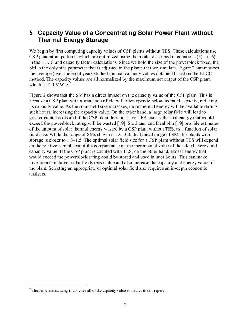
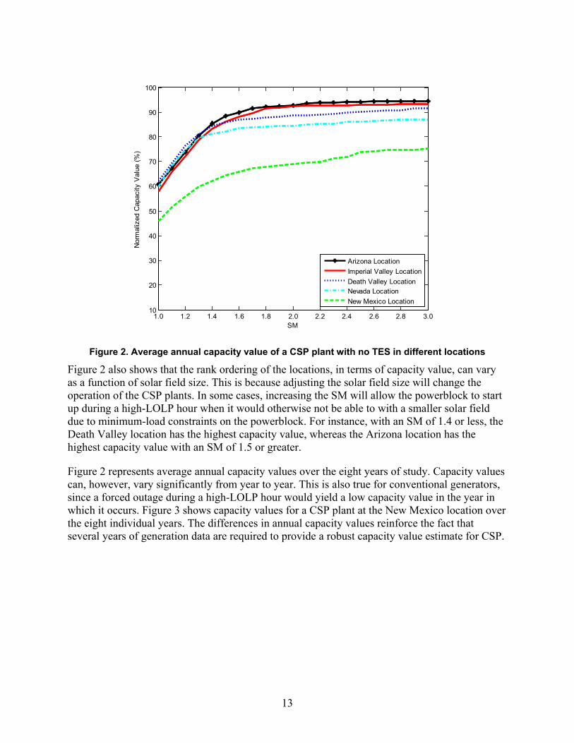
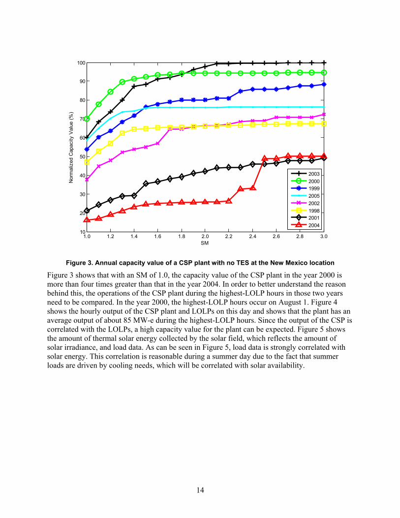
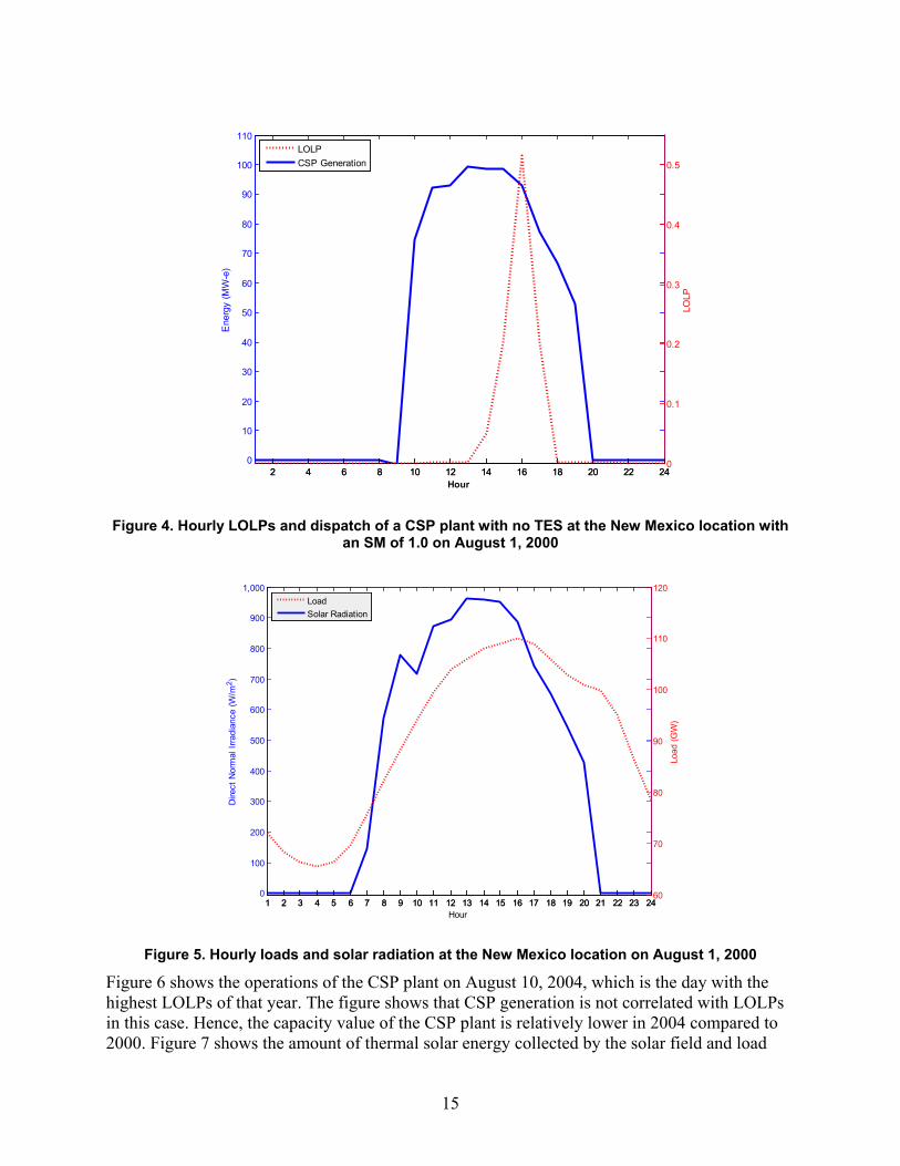
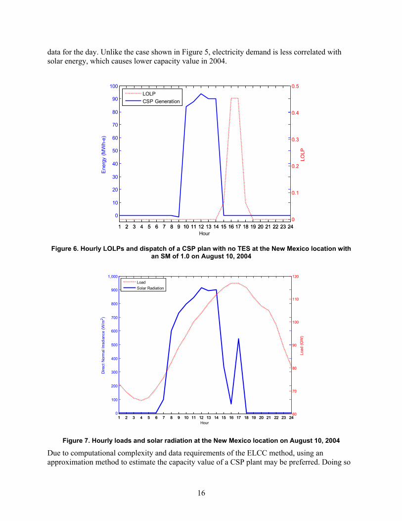
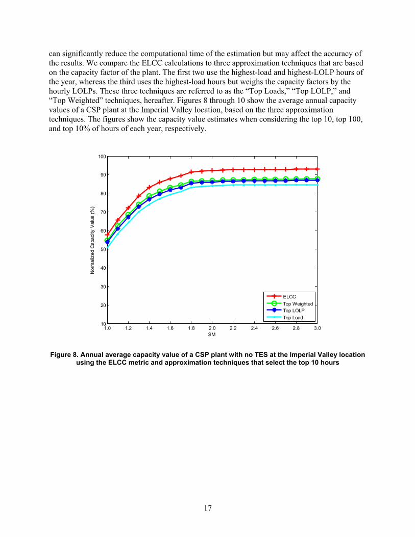
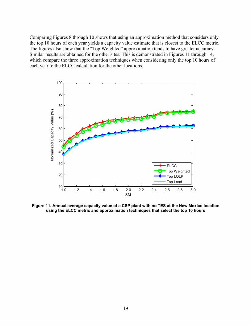
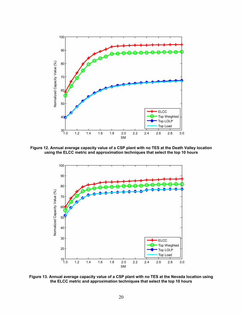
20
10 12 14 16 18 20 22 24 26 28 3030
40
50
60
70
80
90
100
SM
Nor
mal
ized
Cap
acity
Val
ue (
)
ELCCTop WeightedTop LOLPTop Load
Figure 12 Annual average capacity value of a CSP plant with no TES at the Death Valley location
using the ELCC metric and approximation techniques that select the top 10 hours
10 12 14 16 18 20 22 24 26 28 3010
20
30
40
50
60
70
80
90
100
SM
Nor
mal
ized
Cap
acity
Val
ue (
)
ELCCTop WeightedTop LOLPTop Load
Figure 13 Annual average capacity value of a CSP plant with no TES at the Nevada location using
the ELCC metric and approximation techniques that select the top 10 hours
21
10 12 14 16 18 20 22 24 26 28 3010
20
30
40
50
60
70
80
90
100
SM
Nor
mal
ized
Cap
acity
Val
ue (
)
ELCCTop LOLPTop LoadTop Weighted
Figure 14 Annual average capacity value of a CSP plant with no TES at the Arizona location using
the ELCC metric and approximation techniques that select the top 10 hours
51 Effect of Expected Forced Outage Rates on Concentrating Solar Power Capacity Value
Our analysis thus far is based on modeling a system in which the conventional generator set varies from year to year This is because we only model conventional generators that were in operation in each year and this generator set changes from year to year as a result of generator construction and retirements Moreover the EFORs that are reported in the NERC GADS database are annual values which will also vary from year to year depending on how many outages actually occurred We use these annual EFORs to capture the fact that outage rates can vary from year to year These differences in the conventional generator mix and EFORs can contribute to the differences in the annual capacity values of the CSP plants which are shown in Figure 3 Figure 15 compares the average annual ELCC of a CSP plant at the Imperial Valley location in cases in which these parameters vary to a case in which these parameters are held constant In the cases in which the parameters are held constant we use the conventional generator mix that was installed in 2005 and EFORs that are averaged over the eight study years Figure 15 shows that the ELCC values are nearly identical with very little differences for smaller-sized CSP plants The other locations have very similar results As such we can conclude that variations in the mix and reliability of other generators will have a negligible impact on the capacity value of a CSP plant
22
10 12 14 16 18 20 22 24 26 28 3010
20
30
40
50
60
70
80
90
100
SM
Nor
mal
ized
Cap
acity
Val
ue (
)
Different Gen Set and EFORSame Gen Set and EFOR
Figure 15 Average annual capacity value of a CSP plant with no TES at the Imperial Valley location based on ELCC metric with constant and varying conventional generator characteristics
52 Effect of Load Errors on Concentrating Solar Power Capacity Value As noted before another issue with our capacity value estimates is that some utilities do not properly account for daylight savings time in reporting their hourly loads in FERC Form 714 filings As such it is possible that the simulated output of the CSP plant could be offset from the system loads and LOLPs Since the capacity value of CSP is highly dependent on the correlation between solar resource availability and load this potential mismatch in the data can lead to different capacity values than what we have estimated thus far In order to bound the effect of misreported load data we conduct the same ELCC calculations but shift the loads forward and backward one hour Figure 16 shows average annual ELCC values for a CSP plant at the Imperial Valley location when the system loads are shifted in this way and it compares them to the base case in which the reported loads are used without shifting The figure shows that this shifting in the loads can reduce the estimated capacity value of a CSP plant by up to 5 the other locations have similar results The ELCC is reduced regardless of whether the load is shifted forward or backward which suggests that most of the loads reported in the Form 714 data are correct This is because solar resource and CSP generation will have some correlation with system loads and this correlation is maximized when the loads are not shifted
23
10 12 14 16 18 20 22 24 26 28 3010
20
30
40
50
60
70
80
90
100
SM
Nor
mal
ized
Cap
acity
Val
ue (
)
Base CaseShift Load One Hour ForwardShift Load One Hour Backward
Figure 16 Average annual capacity value of a CSP plant with no TES at the Imperial Valley location based on ELCC metric with loads shifted
53 Effect of Sub-Hourly Variability on Concentrating Solar Power Capacity
Value Our analysis thus far is based on using hourly solar data and modeled CSP generation to calculate ELCCs and capacity factors Solar radiation can have noticeable sub-hourly variation due to passing cloud cover Sub-hourly variation may impact the capacity value and integration costs of many renewable resources such as wind and solar PV CSP may not suffer from this issue as much however since the HTF of a CSP plant will have some thermal inertia which can maintain output during a brief reduction in solar radiation Indeed a CSP plant with direct TES will not suffer from short-term transients at all since the powerblock is fed by the TES system and not directly from the solar field
In order to determine the effect of sub-hourly variability on the capacity value of CSP we compare our ELCC calculations when CSP output is modeled using one-minute and hourly data We use one-minute solar data for a CSP plant located around the Nevada One site in Boulder City Nevada The coordinates of the modeled location are 3580o N 11497o W We use one-minute weather data from the year 2007 and compare a case in which the CSP plant is modeled using the one-minute data to a case in which hourly averages of the one-minute data are used instead SAM and the CSP dispatch model are both adapted to model one-minute operations by appropriate scaling of the model variables and parameters The same hourly conventional generator and load data are used in both cases thus any differences in the ELCC estimates are solely due to the one-minute weather data as opposed to hourly averages Since the loads are
24
assumed constant during each hour these ELCC estimates will not capture sub-hourly load variations and potential correlation between these and solar radiation patterns
Figure 17 shows the ELCC estimates for the CSP plant as a function of the solar field size using the one-minute and hourly average data The results show that the hourly average data will provide a close approximation of the ELCC if one-minute data is used The maximum difference in the ELCC between the one-minute and hourly average data is 58 For most plant configurations the hourly average data tends to overestimate the ELCC This is because with one-minute data subhourly variations in solar radiation can keep the powerblock from running above its minimum operating point These variations are not fully captured when the one-minute data is averaged The differences in the estimated ELCCs are maximized for plants with an SM between 24 and 28 This is because plants with this configuration have more time periods in which solar radiation variability can prevent the powerblock from starting up which is not captured without hourly data Despite these issues the small difference in the ELCC values suggest that hourly data can provide relatively good capacity value estimates if sub-hourly data is not available or too computationally intensive to work with
10 12 14 16 18 20 22 24 26 28 3010
20
30
40
50
60
70
80
90
100
SM
Nor
mal
ized
Cap
acity
Val
ue (
)
Hourly Solar DataOne-Minute Solar Data
Figure 17 Capacity value of a CSP plant with no TES at the Boulder City Nevada location based
on ELCC metric while using hourly and one-minute interval solar data
25
6 Capacity Value of a Concentrating Solar Power Plant with Thermal Energy Storage
A major benefit of coupling CSP with TES is that TES will make the CSP plant more dispatchable This is because TES allows the CSP plant to store excess energy collected by the solar field when it is not needed and discharge that energy later when solar resources are lower Our results in Section 5 clearly show that the ability of a CSP plant to generate electricity in critical peak hours with high loads or LOLPs has a significant impact on capacity value Therefore adding TES to a CSP plant can increase its capacity value by allowing it to generate electricity during critical periods when solar resources are not available As suggested earlier adding TES to a CSP plant can also make a higher SM more economic since excess thermal solar energy collected by the solar field will not be wasted and can be stored and later used
Estimating the capacity value of a CSP plant is more complicated when it has a TES system This is because a proper capacity value estimate must not only account for how much energy the plant generates each hour but also how much energy it could produce using energy in storage One must account for energy in storage because if a system shortage event occurs the CSP plant would in principle use energy in storage to help support the system Modeling energy in storage is difficult because of the energy-limited nature of energy storage Namely if energy in TES is used in hour t then it cannot be used in any hour s gt t A previous capacity value estimation technique for energy storage technologies was developed by Tuohy and OrsquoMalley [23] and applied to pumped hydroelectric storage (PHS) Their technique uses operational data to determine the maximum potential output of the PHS device in each hour if the energy in storage is discharged at maximum capacity (based on the available energy in storage) The capacity value of the PHS device is then estimated from the maximum potential output data using a capacity-factor-based approximation technique
We apply a similar approach to estimate the capacity value of the CSP plant with TES As in the case without TES we assume that the operation of the CSP plant and TES is optimized to maximize the revenues that the CSP plant receives Once the operation of the CSP plant is established we can determine the maximum potential output of the CSP plant by first computing the maximum amount of thermal energy that can be delivered from the solar field and TES to the power block in each hour as
1min min (1 ) (17)t t t tSF d l SU umicroτ τ τ φ ρ τ+minus= + minus minus
Equation (17) defines the maximum thermal energy that can be delivered to the powerblock in each hour ( t
microτ ) as the minimum of the powerblockrsquos rated capacity ( +τ τ ) and the sum of thermal energy collected by the solar field and the amount of energy available in TES ( 1min minus+t tSF d lφ ρ ) Equation (17) assumes that if the powerblock is offline it can be committed within the hour in case of a system shortage event [27] We can also define how much of the t
microτ MWh-t is taken from TES as
(18)t t td SFmicro microτ= minus
26
Finally the maximum potential output of the CSP plant etmicro is given by
e ( ) ( ) ( ( )) (19)t t h t b tf P d P fmicro micro micro microτ τ= minus minus
Once we determine the maximum potential output we estimate the capacity value using the top weighted approximation technique considering the 10 highest-load hours of each year since our results in Section 5 show this to be the most accurate approximation
We model the operations of the CSP plant under two different market settings The first is an energy-only market in which the CSP plant only receives payments for the electricity that it supplies to the market The operation of the CSP plant in the energy-only market setting is optimized using the model given in Section 3 and is represented by objective function (6) and constraints (7) through (16) The other market setting that we examine is one in which the CSP plant can receive energy and capacity payments In this case the optimization model must be changed to co-optimize the sum of energy and capacity payments Further details of the capacity payment model are given in Section 62
61 Capacity Value of a Concentrating Solar Power Plant with Thermal Energy Storage in an Energy-Only Market
Figures 18 through 22 summarize the average annual capacity value of CSP plants at the different locations that we study The figures show that the capacity values are typically increasing with the SM and the hours of TES in the CSP plant although this relationship is not perfectly monotonic At all of the locations adding some TES increases the capacity value of the plant above the no-TES case For instance a CSP plant at the New Mexico location with an SM of 15 and no TES has a capacity value of about 78 MW-e Adding one hour of TES to this plant addresses many of the days on which solar and load are not well correlated and increases its capacity value by 47 to 115 MW-e
27
0 2 4 6 8 10 1260
65
70
75
80
85
90
95
100
Hours of TES
Nor
mal
ized
Cap
acity
Val
ue (
)
SM 27
SM 23SM 19
SM 15
Figure 18 Average annual capacity value of a CSP plant with TES at the Imperial Valley location
under an energy-only market setting
0 2 4 6 8 10 1260
65
70
75
80
85
90
95
100
Hours of TES
Nor
mal
ized
Cap
acity
Val
ue (
)
SM 27
SM 23SM 19
SM 15
Figure 19 Average annual capacity value of a CSP plant with TES at the New Mexico location
under an energy-only market setting
28
0 2 4 6 8 10 1260
65
70
75
80
85
90
95
100
Hours of TES
Nor
mal
ized
Cap
acity
Val
ue (
)
SM 27
SM 23SM 19
SM 15
Figure 20 Average annual capacity value of a CSP plant with TES at the Death Valley location
under an energy-only market setting
0 2 4 6 8 10 1260
65
70
75
80
85
90
95
100
Hours of TES
Nor
mal
ized
Cap
acity
Val
ue (
)
SM 27
SM 23SM 19
SM 15
Figure 21 Average annual capacity value of a CSP plant with TES at the Nevada location under an
energy-only market setting
29
0 2 4 6 8 10 1260
65
70
75
80
85
90
95
100
Hours of TES
Nor
mal
ized
Cap
acity
Val
ue (
)
SM 27
SM 23SM 19
SM 15
Figure 22 Average annual capacity value of a CSP plant with TES at the Arizona location under an
energy-only market setting
In some cases however adding an incremental hour of TES or increasing the solar field size may cause a slight reduction in the capacity value of a plant This is because different CSP plant configurations will yield different operational decisions and in some cases a larger CSP plant may have less energy in TES during a high-LOLP hour For example a CSP plant at the Nevada location with four hours of TES and an SM of 22 has a capacity value of 117 MW-e in 1999 The same CSP plant with an SM of 27 would have a lower capacity value of only 95 MW-e in 1999 This difference in the capacity value is due to less energy being in the TES of the larger CSP plant on July 12 which is the day with 5 of the 10 highest hourly LOLPs of the year The larger CSP plant has less energy in storage because the larger solar field provided sufficient energy to operate the powerblock above its minimum operating point in the afternoon of the previous day The smaller solar field of the CSP plant with an SM of 22 could not meet this minimum-load constraint and as such the output of the solar field was stored Thus the CSP plant with an SM of 22 can on average generate up to 74 MW-e during the five highest-LOLP hours on July 12 The larger CSP plant with an SM of 27 can only generate up to an average of 54 MW-e during these hours Figure 23 shows the amount of energy in storage and energy collected by the solar field in each hour on July 12 for these two CSP plant configurations It is important to note that due to weather patterns on this particular day the solar field only collects solar energy during hour 18mdashthe output of the field is zero in the remaining hours
30
Figure 23 LOLP energy from solar field and energy in storage for a CSP plant at the Nevada location with four hours of TES and different SM values on July 12 1999
Adding TES can also in some cases reduce the capacity value of the CSP plant although this is less typical For example a CSP plant at the Death Valley location with an SM of 27 and one hour of TES has a capacity value of 79 MW-e in 1999 Increasing TES by one hour for the same CSP plant reduces its capacity value to 75 MW-e The reduction in capacity value stems from the fact that energy prices are not necessarily correlated with hours with highest LOLPs as suggested by Figure 24 which is a scatter plot of California ISO energy prices and LOLPs in the year 1999 The operation of both of the CSP plants on July 12 which is the day on which the highest LOLPs of the year occur is shown in Figure 25
31
Figure 24 LOLP versus energy price for the Death Valley location in year 1999
Note The x-axis used to represent LOLPs has a logarithmic scale
Figure 25 LOLP energy from solar field and energy in storage for a CSP plant at the Death Valley
location with an SM of 27 and different TES sizes on July 12 1999
32
Figure 25 shows that in hour 16 during which the LOLP is the highest the larger CSP plant has less energy in storage compared to the smaller CSP plant This reduces the capacity value of the larger CSP plant The reason behind these operations is that in hours 12 through 15 of the day the larger CSP plant will use energy in TES to generate electricity since energy prices are higher in these hours than in hours during which the highest LOLPs occur The smaller CSP cannot do so since its smaller TES system does not have sufficient energy in storage to operate above its minimum generation point during these hours These operational differences leave the smaller CSP plant with more energy in TES during hour 16 which yield the higher capacity value
62 Capacity Value of a Concentrating Solar Power Plant with Thermal Energy Storage in a Capacity Market
In Section 61 we estimate the capacity value of a CSP plant with TES in an energy-only market The results there suggest that adding TES to a CSP plant will tend to increase the capacity value of the plant although this relationship is not monotonic This is because energy prices and LOLPs will not always be perfectly correlated and there can be high-LOLP hours that have lower energy prices than other hours with lower LOLPs An example of this is demonstrated in Figure 25 An alternative market design that could help reduce the impact of such price and LOLP patterns is an energy and capacity market Under such a market design the CSP plant receives both payments for electricity that it generates as well as the capacity that it provides the system Many electricity markets have moved toward adopting capacity markets Even in systems that do not have an explicit capacity market such as the APS NP and PNM service territories a model that maximizes the sum of energy and capacity payments may be more appropriate This is because such integrated utilities would likely operate a CSP plant to minimize its overall energy supply costsmdashwhich would be akin to our energy revenue maximization However such utilities would also likely adjust the operation of their plants to have more energy available in TES during anticipated system shortage events
The introduction of a capacity market tends to increase the capacity value of a CSP plant since capacity payments typically have performance requirements that are related to the capacity value of a generator Most capacity markets impose financial penalties on generators that do not meet the performance requirements Although the specific performance requirements differ from market to market they are typically related to how much firm capacity a generator has available during system shortage events Our capacity market model is based on the forward capacity market (FCM) used by ISO New England although the modeling framework is sufficiently general that it can be adapted to model other markets as well
621 Capacity Market Procedures The objective of a capacity market is to encourage enough generating capacity to enter the system so that reliability requirements are met This objective is met by a forward capacity auction (FCA)8
8 These auctions are held three years in advance for ISO New Englandrsquos FCM
Resources that participate and are selected in the FCA are eligible to receive capacity payments throughout the capacity commitment period based on their capacity commitment obligations Capacity payments are subject to certain performance requirements however Performance requirements are set so that the capacity resources contribute to system reliability during hours in which shortage events could occur The definition of shortage events will differ between capacity markets Some markets such as the FCM define shortage events as
33
periods during which reserves (spinning and non-spinning reserves) fall below certain levels This definition does not necessarily imply that supply is less than demand during the shortage event hours For instance if the reserve level falls to 1 generating capacity will still be greater than demand but due to low reserve levels the probability of having a capacity deficiency is high Based on this definition there is a one-to-one relationship between shortage event hours and the hourly LOLPs In this study the 10 hours of each year with the highest LOLPs are defined as shortage event hours
A generator that fails to provide its contracted capacity during a shortage event hour will incur financial penalties The FCM sets penalties based on the cost of replacement capacity We assume that the capacity market uses the cost of a natural-gas-fired combustion turbine which we assume to be $671kW in 2008 dollars to set the penalties This cost is then translated into an annualized cost of $7381kW-year using an 11 capital charge rate We assume that the capacity market imposes a penalty that is equal to half of this annualized cost which is reflective of the penalties imposed in the FCM We use consumer price index data to deflate the cost of the combustion turbine to previous-year dollars
622 Optimization Model In order to determine the operations of a CSP plant in an energy- and capacity-market setting our model must be adjusted to maximize the sum of energy and capacity payments and net of any capacity penalties We follow a similar approach to that used in Section 61 and add variables to our optimization model that determine the maximum potential generation from the CSP plant in each hour (based on energy in TES and collected by the solar field) The difference between the firm capacity sold and this maximum potential generation is the shortfall from the capacity commitment and these shortfalls are penalized in the objective function to reflect capacity penalties In order to give the formulation of the model we define the following parameters
Market clearing price of capacity ($MW-year) Penalty factor for unserved capacity requirements
Set of hours during which shortage events occur
cMPFH
We also define the following variables
Firm capacity sold
e Maximum potential net electric energy (MWh-e) produced by powerblock in each hoursold
t
Cmicro
Maximum potential thermal energy taken out of storage (MWh-t) in each hour
Maximum potential total thermal energy (MWh-t) fed to powerblock in each hour
Shortfall from capacity commit
t
tshortt
d
C
micro
microτ
ment in each hour
The formulation of the model is then given by
max short
e c c tt t sold
t T t H sold
C( M c )e M C ( M PF )
Cisin isin
minus + minussum sum (20)
34
st (7)-(16) e short
t sold tC C microge minus t Tforall isin (21)
1 t td lmicro ρ minusle t Tforall isin (22) t t t td SU r SFmicro microφ τ τminus + + le t Tforall isin (23)
e t t h t b tf ( ) P ( d ) P ( f ( ))micro micro micro microτ τ= minus minus t Tforall isin (24)
t t t u umicroτ τ τ τ τminus +le le t Tforall isin (25)
Objective function (20) maximizes the sum of net energy and capacity revenues The last term in the objective function corresponds to penalties associated with shortfalls from capacity commitments Constraints (7) through (16) which are from the original energy-only model are included since the same underlying constraints on the operation of the CSP plant apply Constraint (21) defines the hourly capacity commitment shortfall as the difference between firm capacity sold and the maximum potential net electrical generation of the CSP plant Constraint (22) restricts the potential thermal energy taken out of storage (MWh-t) in each hour based on the ending storage level of the previous hour Constraint (23) limits the total amount of potential thermal energy used in the CSP plant to not be greater than the energy collected by the solar field Constraint (24) defines the maximum potential output of the CSP plant in each hour Finally constraint (25) imposes restrictions on potential capacity of the CSP plant when the powerblock is online
Because the penalty term in the objective function is non-linear in the variables we solve this model by fixing the value of Csold and solving the model iteratively until finding a maximum For the cases that we consider selling 120 MW-e of capacity (the maximum net output of the CSP plant) maximizes CSP revenues
623 Results The model given by objective function (20) and constraints (7) through (16) and (21) through (25) is used to determine the optimized operation of the CSP plant in each hour We then apply the same capacity-factor-based approximation technique used in Section 61 to estimate the capacity value of the plant Figures 26 through 30 summarize the average annual capacity value of the CSP plants at the different locations
35
0 2 4 6 8 10 1260
65
70
75
80
85
90
95
100
Hours of TES
Nor
mal
ized
Cap
acity
Val
ue (
)
SM 27
SM 23SM 19
SM 15
Figure 26 Average annual capacity value of a CSP plant with TES at the Imperial Valley location
under an energy and capacity market setting
0 2 4 6 8 10 1260
65
70
75
80
85
90
95
100
Hours of TES
Nor
mal
ized
Cap
acity
Val
ue (
)
SM 27
SM 23SM 19
SM 15
Figure 27 Average annual capacity value of a CSP plant with TES at the New Mexico location
under an energy and capacity market setting
36
0 2 4 6 8 10 1260
65
70
75
80
85
90
95
100
Hours of TES
Nor
mal
ized
Cap
acity
Val
ue (
)
SM 27
SM 23SM 19
SM 15
Figure 28 Average annual capacity value of a CSP plant with TES at the Death Valley location
under an energy and capacity market setting
0 2 4 6 8 10 1260
65
70
75
80
85
90
95
100
Hours of TES
Nor
mal
ized
Cap
acity
Val
ue (
)
SM 27
SM 23SM 19
SM 15
Figure 29 Average annual capacity value of a CSP plant with TES at the Nevada location under an
energy and capacity market setting9
9 The unusual result for Nevada (compared to the other locations) is due to a day in 1999 where an SM of less than 27 was insufficient to meet the minimum generation requirement during one 3-hour period of high LOLP This demonstrates the need to examine performance over a large period of time to examine the impact of variability on resource adequacy
37
0 2 4 6 8 10 1260
65
70
75
80
85
90
95
100
Hours of TES
Nor
mal
ized
Cap
acity
Val
ue (
)
SM 27
SM 23SM 19
SM 15
Figure 30 Average annual capacity value of a CSP plant with TES at the Arizona location under an
energy and capacity market setting
Figures 26 through 30 show the benefits of implementing a capacity payment scheme as opposed to an energy-only market Adding capacity payments tends to slightly increase the capacity value of the CSP plant Moreover the capacity value is more monotonic in the size of the plant There are still however some cases in which increasing the size of a CSP plant can result in a slight reduction in the capacity value Even when the capacity payment is added there may still be high-LOLP hours in which the value of energy (when accounting for the energy price and capacity penalty) is lower than other hours with lower LOLPs However these cases are rare and their magnitude (in terms of capacity value reductions) is relatively small
More broadly contrasting these results with the energy-only market design and Figure 23 in particular demonstrates the benefit of capacity payments (or co-optimizing the energy and capacity value of a CSP plant) in improving the system benefits of CSP Figure 23 shows that the larger CSP plant has a lower capacity value because of poor correlation between energy prices and LOLPs and the lack of solar resource during high-LOLP hours If a CSP plant can anticipate potential high-LOLP periods or shortage events the total value of the plant to the system can be drastically increased by slightly adjusting plant operations
38
7 Conclusions
This study estimates the capacity value of a CSP plant at a variety of locations within the WECC while accounting for rational dispatch behavior of a CSP operator This is done by optimizing the operation of the CSP plant and by using standard reliability-based capacity value estimation techniques Although the ELCC metric is the most accurate estimation technique we show that capacity-factor-based approximation methods can closely estimate the ELCC value
When introducing TES the capacity value of the CSP plant is more difficult to estimate since one must account for energy in storage We apply the capacity-factor-based technique used by Tuohy and OrsquoMalley [23] under two different market settings an energy-only market and an energy and capacity market Our results show that adding TES to a CSP plant can increase its capacity value significantly at all of the locations Adding a single hour of TES significantly increases the capacity value above the no-TES case in most cases to above 90 Although additional hours of TES increase the capacity value of the plant their marginal benefit is less than the first hour of TES Nevertheless Sioshansi and Denholm [19] show that a greater number of hours of TES can have incremental energy and ancillary service benefits Since energy prices LOLPs and solar resource will not be perfectly correlated the use of capacity payments (or co-optimization of energy and capacity value) can significantly increase the value of a CSP plant to the power system compared to an energy-only market
The capacity value estimates we provide examine a single CSP plant which will have a marginal effect on the rest of the system Clearly changes in the generation mix or load patterns could affect the capacity value of a CSP plant Adding more CSP (or PV) plants especially if they are concentrated at similar locations in the system can reduce the marginal capacity value of additional CSP capacity Adding TES to a CSP plant can alleviate this reduction in the marginal capacity value however since it gives the CSP plant additional flexibility in dispatching its generation
39
References
[1] Soumlder L Amelin M ldquoA Review of Different Methodologies Used for Calculation of Wind Power Capacity Creditrdquo Proceedings of the IEEE Power Engineering Society General Meeting 2008 Pittsburgh PA 2008
[2] Pudaruth GR Li F Capacity Credit Evaluation A Literature Review Third International Conference on Electric Utility Deregulation and Restructuring and Power Technologies DRPT 2008 Nanjing China pp 2719ndash2724
[3] Milligan M Porter K ldquoDetermining the Capacity Value of Wind An Updated Survey of Methods and Implementationrdquo WindPower 2008 June 2008 Houston Texas
[4] Billinton R Allan R Reliability Evaluation of Power Systems 2nd edition New York Plenum Press 1984
[5] Kahn EP ldquoEffective Load Carrying Capability of Wind Generation Initial Results with Public Datardquo The Electricity Journal Vol 17 Iss 10 December 2004 pp 85ndash95
[6] Amelin M ldquoComparison of Capacity Credit Calculation Methods for Conventional Power Plants and Wind Powerrdquo IEEE Trans Power Syst Vol 24 No 2 May 2009
[7] Ensslin C Milligan M Holttinen H OrsquoMalley M Keane A ldquoCurrent Methods to Calculate Capacity Credit of Wind Power IEA collaborationrdquo Proceedings 2008 IEEE Power amp Energy Society General Meeting 2008 p 3
[8] Milligan M Parsons B ldquoA Comparison and Case Study of Capacity Credit Algorithms for Intermittent Generatorsrdquo Proceedings Solar rsquo97 April 27ndash30 1997 Washington DC NRELCP-440-22591 Golden CO National Renewable Energy Laboratory March 1997
[9] Keane A Milligan M DAnnunzio C Dent CJ Dragoon K Hasche B Holttinen H Samaan N Sumloder L OMalley M ldquoCapacity Value of Wind Powerrdquo IEEE Trans Power Syst forthcoming
[10] DrsquoAnnunzio C Santoso S ldquoNoniterative Method to Approximate the Effective Load Carrying Capability of a Wind Plantrdquo IEEE Trans Energy Conv Vol 23 No 2 June 2008 pp 544ndash550
[11] Martin B Diesendorf M ldquoCalculating the Capacity Credit of Wind Powerrdquo Proceedings 4th Biennial Conference University of Queensland August 1980 Brisbane Queensland Australia pp 36ndash42
[12] Garver LL ldquoEffective Load Carrying Capability of Generating Unitsrdquo IEEE Trans on PAS Vol PAS-85 August 1966 pp 910ndash919
[13] Hoff T Perez R Ross JP Taylor M ldquoPhotovoltaic Capacity Valuation Methodsrdquo SEPA REPORT 02-08 Washington DC Solar Electric Power Association 2008
40
[14] Bernow S Biewald B Singh D ldquoModelling Renewable Electric Resources A Case Study of Wind Reliabilityrdquo Presented at the NARUC-DOE National Conference on Renewable Energy Savannah GA October 1993
[15] El-Sayed M ldquoSubstitution Potential of Wind Energy in Egyptrdquo Energy Policy Vol 30 2002 pp 681ndash687
[16] Milligan M Parsons B ldquoA Comparison and Case Study of Capacity Credit Algorithms for Wind Power Plantsrdquo Wind Energy Vol 23 Iss 3 1999 pp 159ndash166
[17] Milligan M Porter K ldquoThe Capacity Value of Wind in the United States Methods and Implementationrdquo The Electricity Journal Vol 19 Iss 2 March 2006
[18] Milligan M Modeling Utility-scale Wind Power Plants Part 2 Capacity Credit NRELTP-500-27514 Golden CO National Renewable Energy Laboratory June 2000
[19] Sioshansi R Denholm P ldquoThe Value of Concentrating Solar Power and Thermal Energy Storagerdquo IEEE Trans Sustainable Energy Vol 1 October 2010 pp 173ndash183
[20] Gilman P Blair N Mehos M Christensen C Janzou S Solar Advisor Model User Guide for Version 20 NRELTP-670-43704 Golden CO National Renewable Energy Laboratory August 2008
[21] Pacheco JE Gilbert R Overview of Recent Results of the Solar Two Test and Evaluations Programrdquo SAND99-0091C Albuquerque NM Sandia National Laboratories January 1999
[22] Herrmann U Kelly B Price H ldquoTwo-tank Molten Salt Storage for Parabolic Trough Solar Power Plantsrdquo Energy Vol 29 AprilndashMay 2004 pp 883ndash893
[23] Tuohy A OrsquoMalley M ldquoImpact of Pumped Storage on Power Systems with Increasing Wind Penetrationrdquo Power amp Energy Society General Meeting July 26ndash30 2009 Calgary AB Canada Institute of Electrical and Electronics Engineers pp 1ndash8
[24] US Department of Energy Form 860 httpwwweiadoegovcneafelectricitypageeia860html Accessed June 20 2011
[25] North American Electric Reliability Corporation Generating Availability Data System httpwwwnerccompagephpcid=4|43 Accessed June 20 2011
[26] Federal Energy Regulatory Commission Form No 714 httpwwwfercgovdocs-filingformsform-714elec-subm-softasp Accessed June 20 2011
[27] Ho CK Kolb GJ ldquoIncorporating Uncertainty into Probabilistic Performance Models of Concentrating Solar Power Plantsrdquo J Sol Energy Eng Vol 132 Iss 3 August 2010
- Acknowledgments
- List of Acronyms
- Executive Summary
- Table of Contents
- List of Figures
- List of Tables
- 1 Introduction
- 2 Methods for Estimating Capacity Value
-
- 21 Effective Load Carrying Capability
- 22 Approximation Methods
-
- 3 Concentrating Solar Power Model
- 4 Data Requirements
- 5 Capacity Value of a Concentrating Solar Power Plant without Thermal Energy Storage
-
- 51 Effect of Expected Forced Outage Rates on Concentrating Solar Power Capacity Value
- 52 Effect of Load Errors on Concentrating Solar Power Capacity Value
- 53 Effect of Sub-Hourly Variability on Concentrating Solar Power Capacity Value
-
- 6 Capacity Value of a Concentrating Solar Power Plant with Thermal Energy Storage
-
- 61 Capacity Value of a Concentrating Solar Power Plant with Thermal Energy Storage in an Energy-Only Market
- 62 Capacity Value of a Concentrating Solar Power Plant with Thermal Energy Storage in a Capacity Market
-
- 7 Conclusions
- References
-
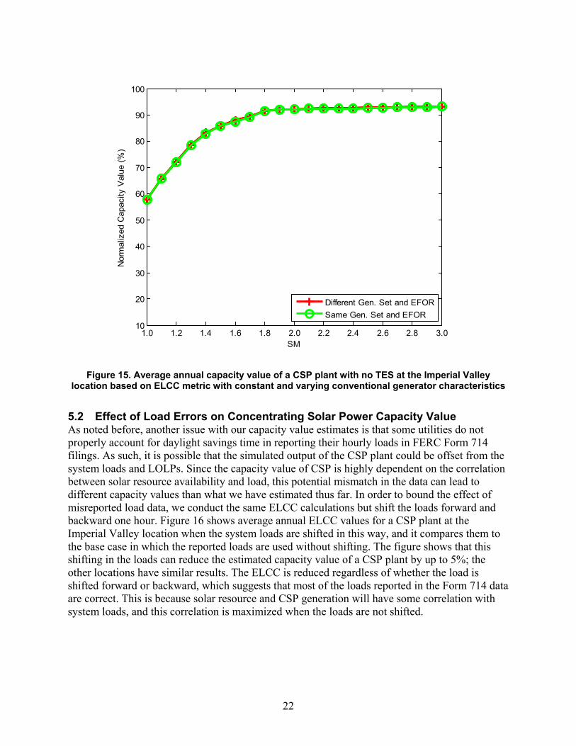
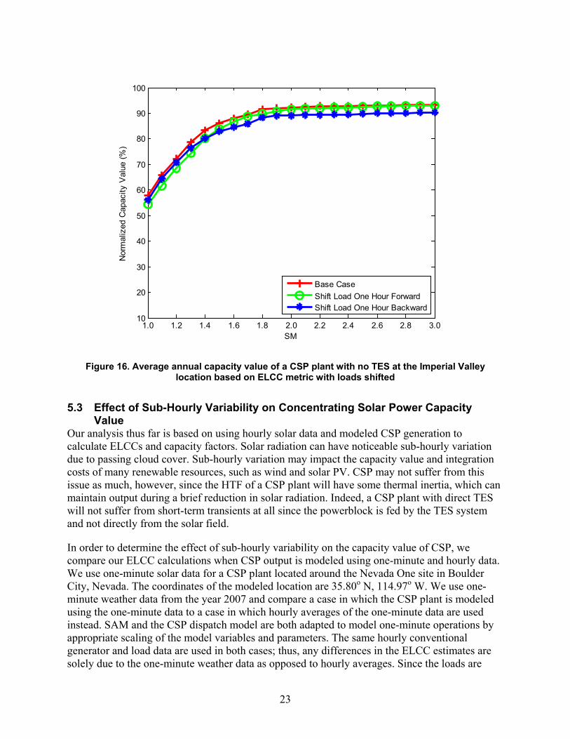
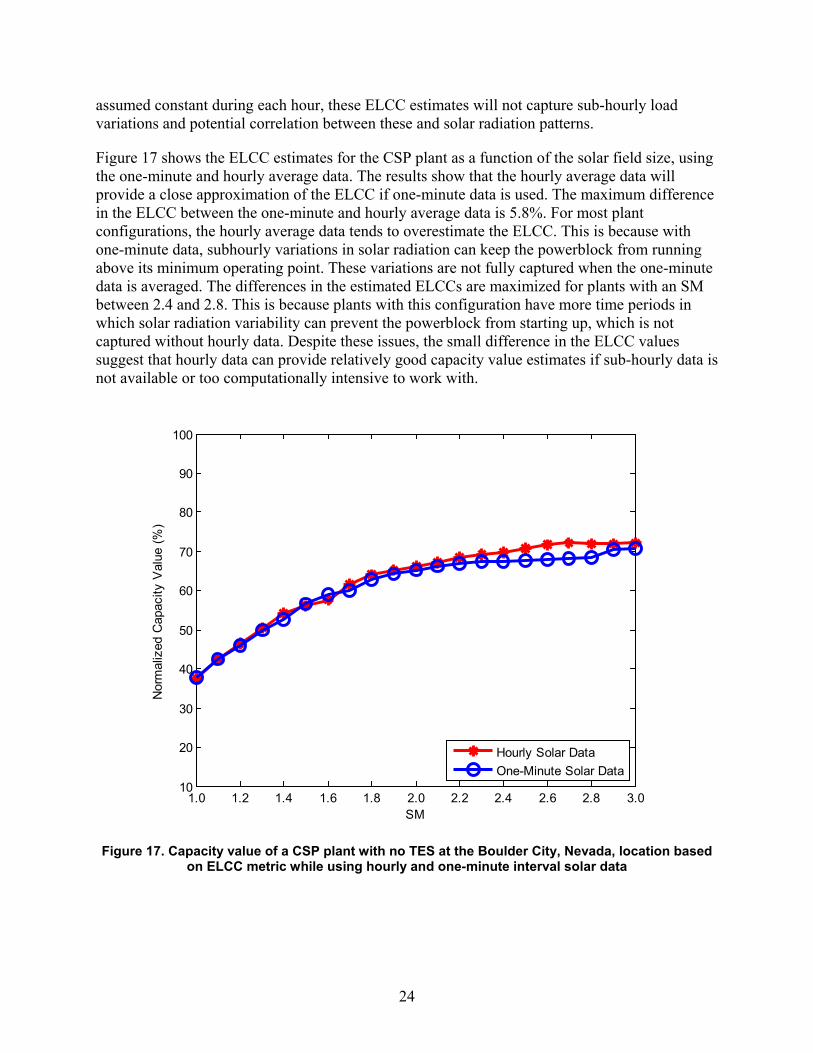
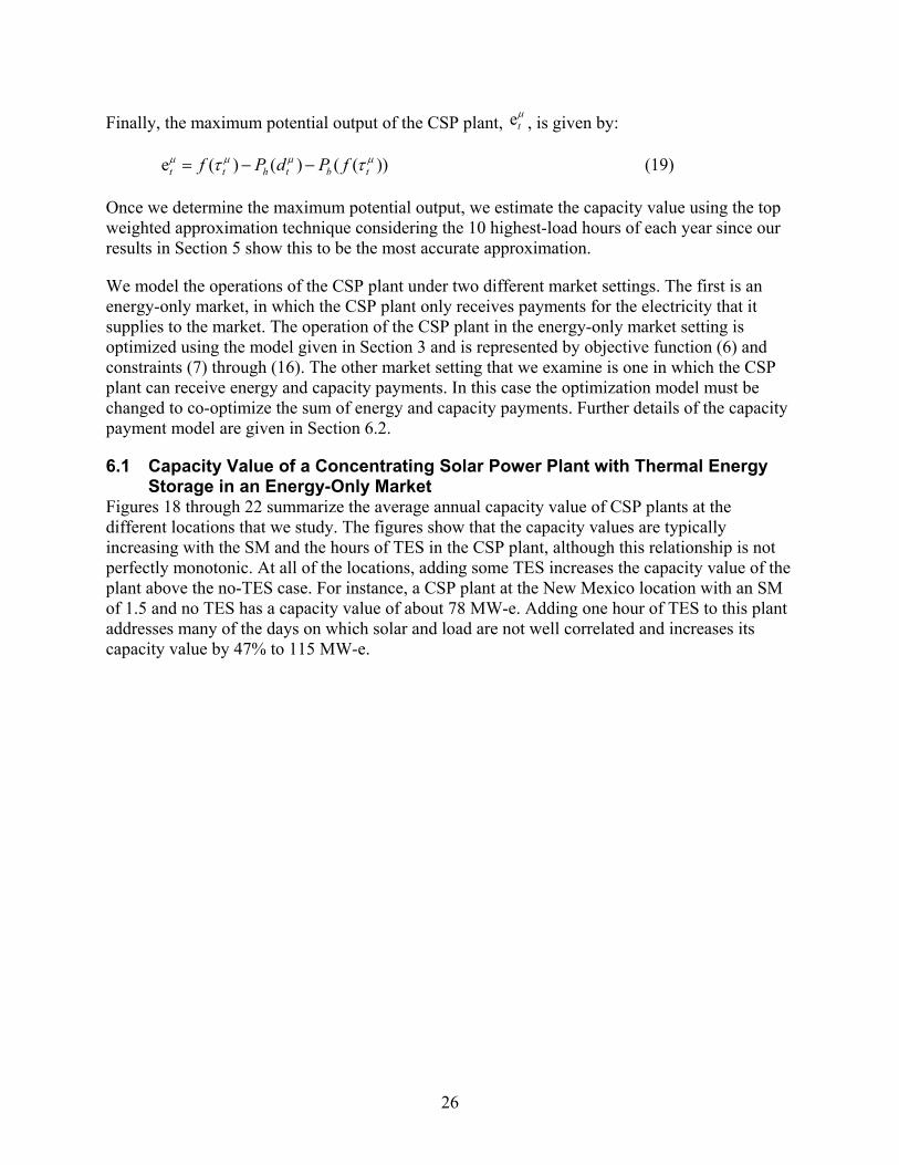
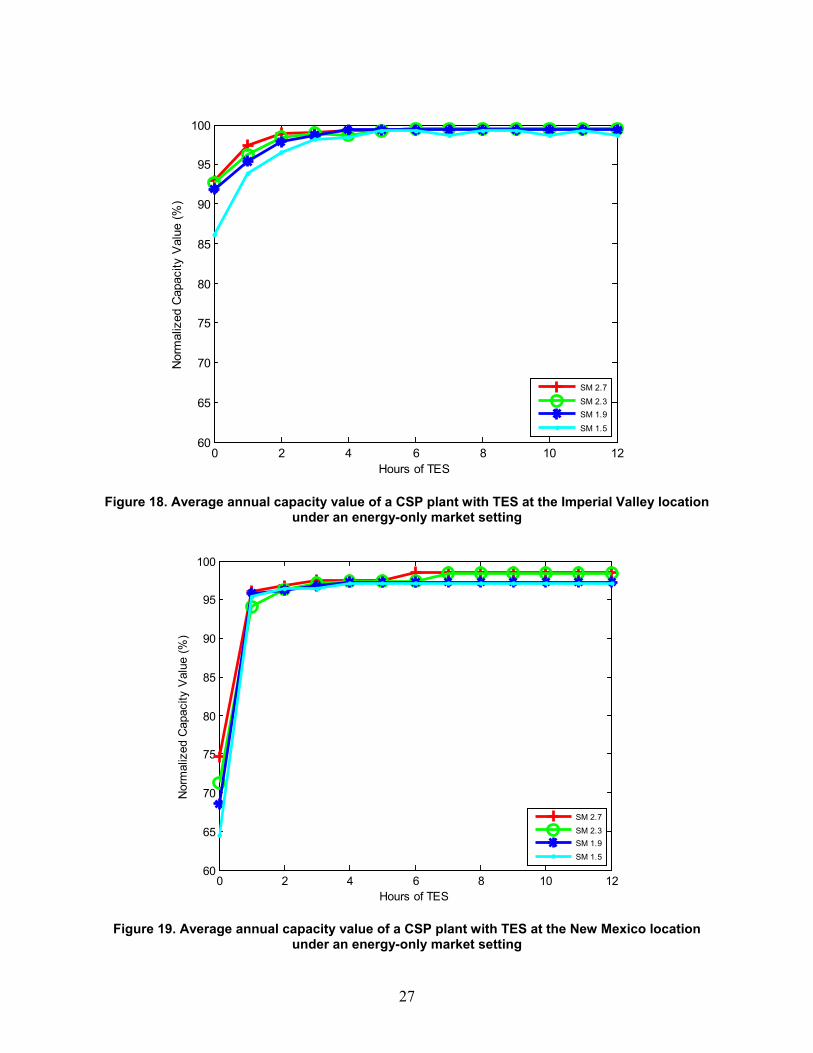
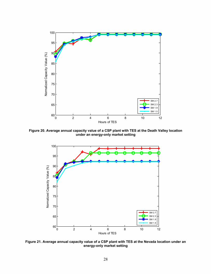
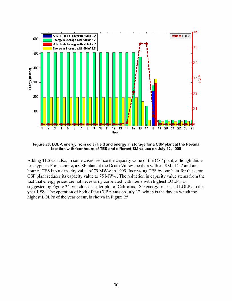
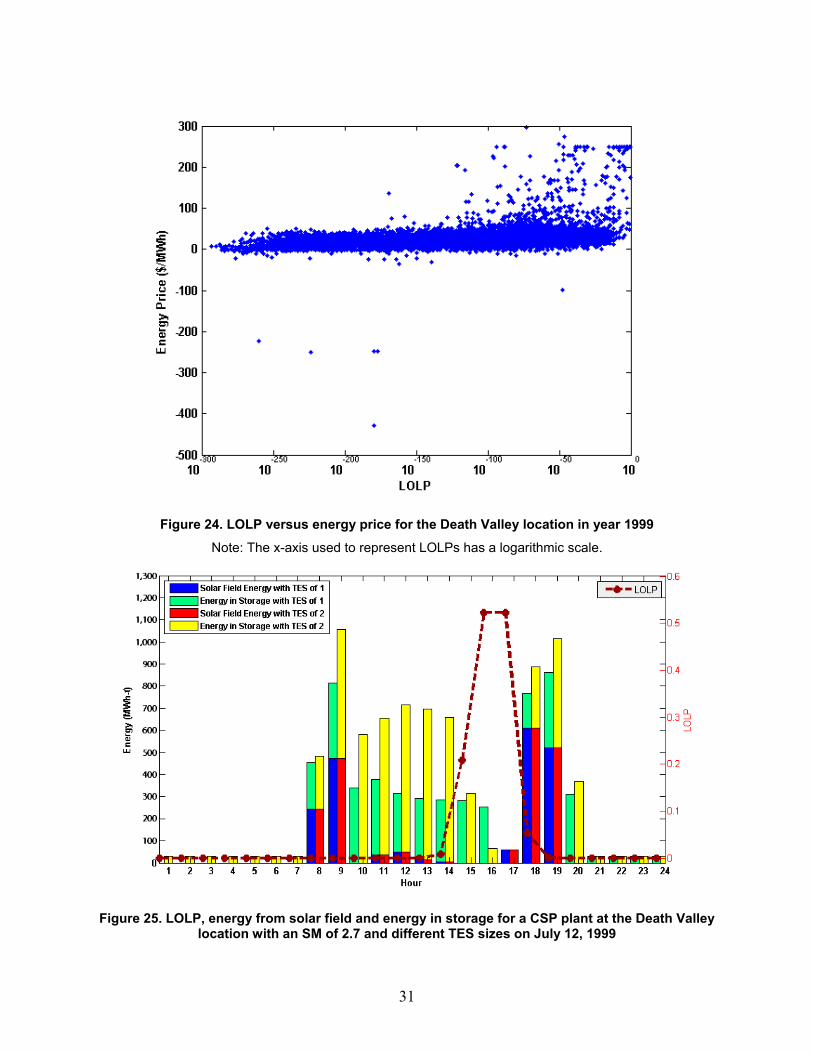
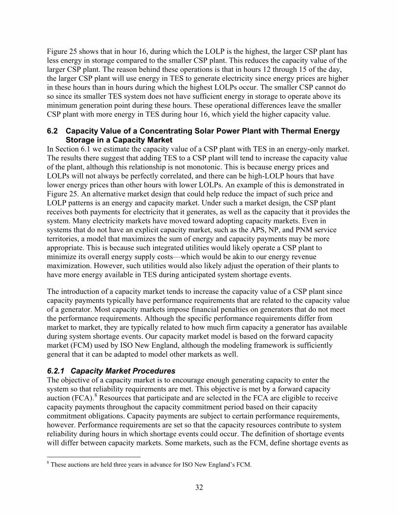
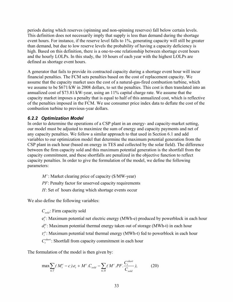
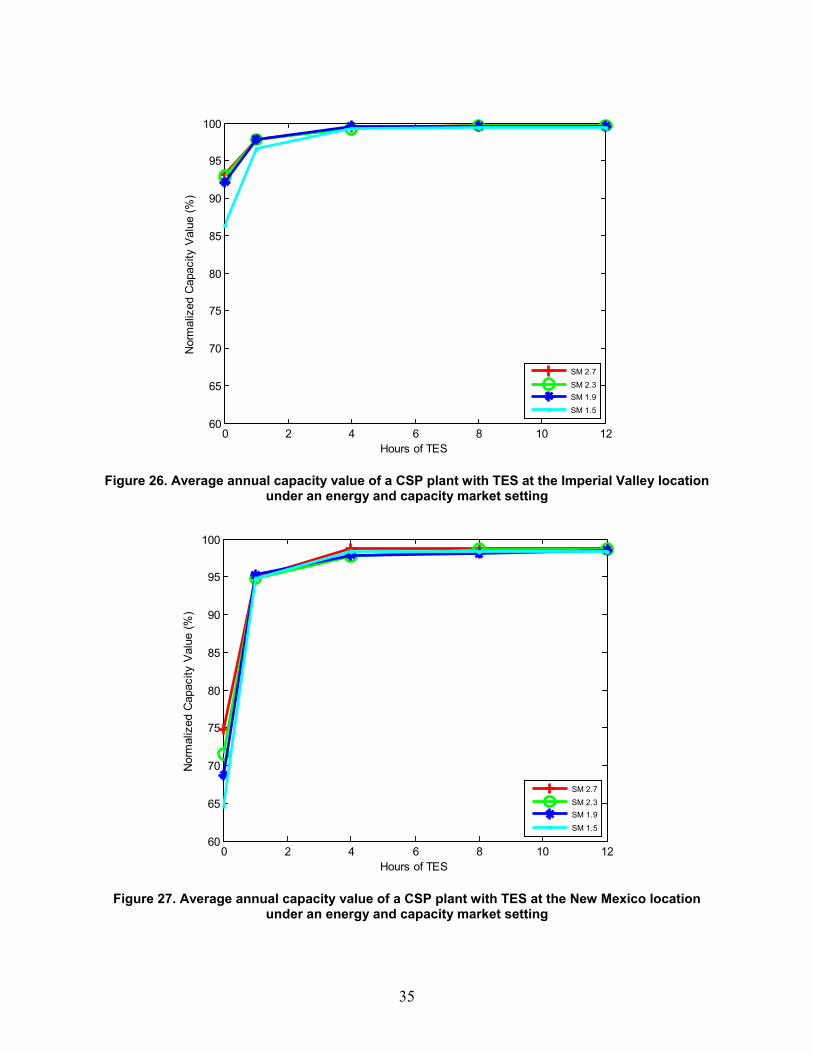
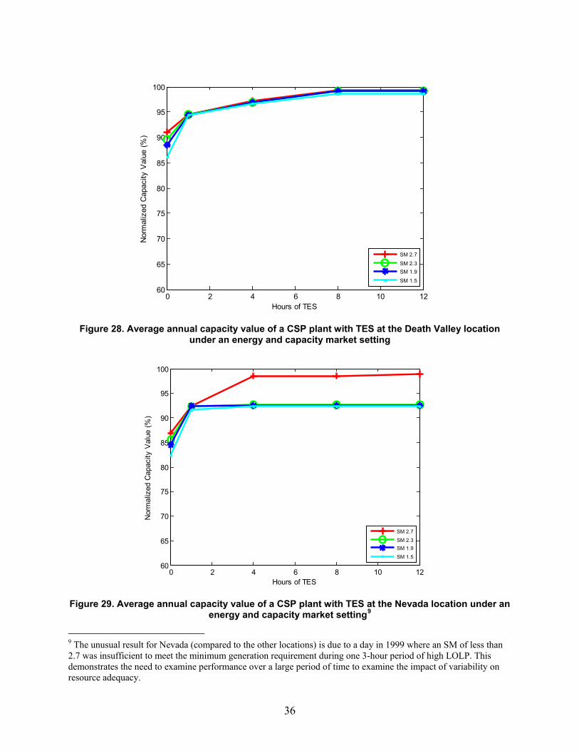
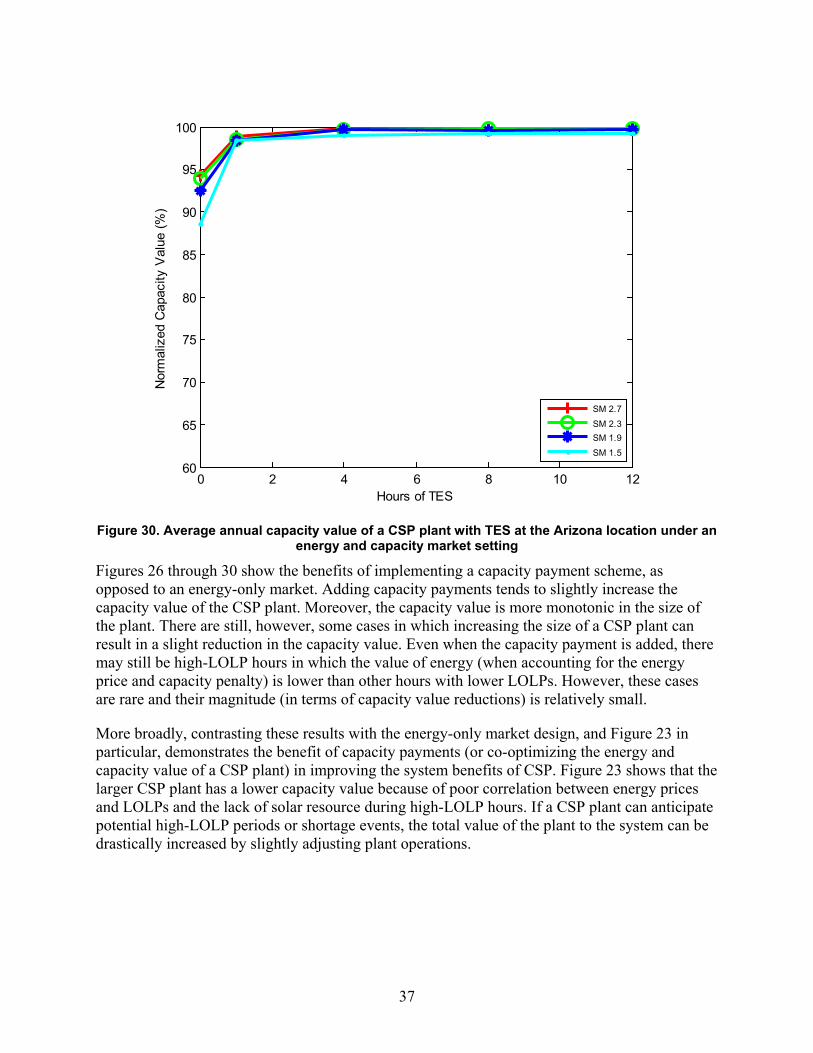