CAP 5993/CAP 4993 Game Theory
59
Transcript of CAP 5993/CAP 4993 Game Theory

2
Announcements
• HW1
• HW2
• midterm

3
Extensive-form game
• A game in extensive form is given by a game tree, which
consists of a directed graph in which the set of vertices
represents positions in the game, and a distinguished vertex,
called the root, represents the starting position of the game. A
vertex with no outgoing edges represents a terminal position in
which play ends. To each terminal vertex corresponds an
outcome that is realized when the play terminates at that vertex.
Any nonterminal vertex represents either a chance move (e.g., a
toss of a die or a shuffle of a deck of cards) or a move of one of
the players. To any chance-move vertex corresponds a
probability distribution over edges emanating from that vertex,
which correspond to the possible outcomes of the chance move.

4

5
Perfect vs. imperfect information
• To describe games with imperfect information, in
which players do not necessarily know the full board
position (like poker), we introduce the notion of
information sets. An information set of a player is a set
of decision vertices of the player that are
indistinguishable by him given his information at that
stage of the game. A game of perfect information is a
game in which all information sets consist of a single
vertex. In such a game whenever a player is called to
take an action, he knows the exact history of actions
and chance moves that led to that position.

6
• A strategy of a player is a function that assigns to each
of his information sets an action available to him at that
information set. A path from the root to a terminal
vertex is called a play of the game. When the game has
no chance moves, any vector of strategies (one for each
player) determines the play of the game, and hence the
outcome. In a game with chance moves, any vector of
strategies determines a probability distribution over the
possible outcomes of the game.

7

8
• Theorem (von Neumann [1928]) In every two-
player game (with perfect information) in which
the set of outcomes is O = {Player 1 wins,
Player 2 wins, Draw}, one and only one of the
following three alternatives holds:
1. Player 1 has a winning strategy.
2. Player 2 has a winning strategy.
3. Each of the two players has a strategy
guaranteeing at least a draw.

9
Chance moves
• In the games we have seen so far, the transition from one state to another is
always accomplished by actions undertaken by the players. Such a model is
appropriate for games such as chess and checkers, but not for card games or
dice games (such as poker or backgammon) in which the transition from one
state to another may depend on a chance process: in card games, the shuffle
of the deck, and in backgammon, the toss of the dice. It is possible to come
up with situations in which transitions from state to state depend on other
chance factors, such as the weather, earthquakes, or the stock market. These
sorts of state transitions are called chance moves. To accommodate this
feature, our model is expanded by labeling some of the vertices in the game
tree (V, E, x0) as chance moves. The edges emanating from vertices
corresponding to chance moves represent the possible outcomes of a lottery,
and next to each such edge is listed the probability that the outcome it
represents will be the result of the lottery.

10
Rock-paper-scissors
0,0 -1,1 0,0 0,0-1,1 -1,11,-1 1,-1 1,-1

11
Strategies in imperfect-information games
• A strategy of player i is a function from each of
his information sets to the set of actions
available at that information set.
• Just as in games with chance moves and perfect
information, a strategy vector determines a
distribution over the outcomes of a game.

12
• Theorem (Kuhn) Every finite game with perfect
information has at least one pure strategy Nash
equilibrium.
• Corollary of Nash’s Theorem: Every extensive-form
game (of perfect or imperfect information) has an
equilibrium in mixed strategies.
13
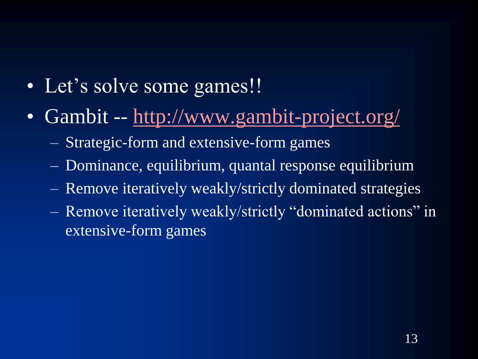
• Let’s solve some games!!
• Gambit -- http://www.gambit-project.org/– Strategic-form and extensive-form games
– Dominance, equilibrium, quantal response equilibrium
– Remove iteratively weakly/strictly dominated strategies
– Remove iteratively weakly/strictly “dominated actions” in
extensive-form games

14
Quantal response equilibrium
• Quantal response equilibrium (QRE) provides an equilibrium
notion with bounded rationality. QRE is not an equilibrium
refinement, and it can give significantly different results from
Nash equilibrium.
• In a quantal response equilibrium, players are assumed to make
errors in choosing which pure strategy to play. The probability
of any particular strategy being chosen is positively related to
the payoff from that strategy. In other words, very costly errors
are unlikely.
• The equilibrium arises from the realization of beliefs. A player's
payoffs are computed based on beliefs about other players'
probability distribution over strategies. In equilibrium, a player's
beliefs are correct.

15
• By far the most common specification for QRE is logit
equilibrium (LQRE).
• Pij is probability of player i choosing strategy j.
• The parameter λ is non-negative (sometimes written as 1/μ).
• λ can be thought of as the rationality parameter. As λ→0, players
become "completely non-rational", and play each strategy with
equal probability. As λ→∞, players become "perfectly rational,"
and play approaches a Nash equilibrium.

16
Dominance
– Remove iteratively weakly/strictly dominated
strategies
– Remove iteratively weakly/strictly “dominated
actions” in extensive-form games

17
• Compute one Nash equilibrium
– Solving Linear program
– Simplicial subdivision
– Tracing logit equilibria
18
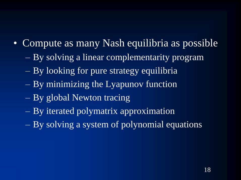
• Compute as many Nash equilibria as possible
– By solving a linear complementarity program
– By looking for pure strategy equilibria
– By minimizing the Lyapunov function
– By global Newton tracing
– By iterated polymatrix approximation
– By solving a system of polynomial equations

19
• Compute all Nash equilibria
– By enumerating extreme points

20
Extensive-form games
• Compute one Nash equilibrium
– Using the extensive-form game
– Using the strategic-form game
• Some of the algorithms appropriate for just extensive
vs. strategic form

21
Prisoner’s dilemma
C D
C 4, 4 0, 5
D 5, 0 1, 1

22
Battle of the sexes

23
Rock-paper-scissors
rock paper scissors
Rock 0,0 -1, 1 1, -1
Paper 1,-1 0, 0 -1,1
Scissors -1,1 1,-1 0,0

24
Security game

25
Chicken

26
Rock-paper-scissors
0,0 -1,1 0,0 0,0-1,1 -1,11,-1 1,-1 1,-1

27

28
WL/12 CC CF FC FF
00 0 0 0 0
01 -0.5 -0.5 1 1
02 -1 1 -1 1
10 …
11
12
20
21
22

29
• “Because of the field’s widespread applicability and the variety of
mathematical and computational issues it encompasses, it is hard to place
game theory within any single discipline (although it has traditionally been
viewed as a branch of economics). While the field is clearly benefitting from
being analyzed from many different perspectives, it is also important to make
sure that it doesn’t become disorganized as a result. When I started doing
research for my thesis, I was surprised at how difficult it was to find a basic
introduction to the fundamental mathematical and computational results. I
had to turn to game theory textbooks for proofs of classical results, operations
research and optimization books for results in linear programming and linear
complementarity, and more recent computer science and economics papers
for algorithms and complexity results. Thus, the major contribution of this
paper is to present the basic mathematical and computational results related
to computing Nash equilibria in a coherent form that can benefit people from
all fields.”
• http://www.cs.cmu.edu/~sganzfri/SeniorThesis.pdf

30
Computing Nash equilibria of two-
player zero-sum games
• Consider the game G = ({1,2}, A1 x A2, (u1, u2)).
• Let U*i be the expected utility for player i in equilibrium (the
value of the game); since the game is zero-sum, U*1 = - U*2.
• Recall that the Minmax Theorem tells us that U*1 holds constant
in all equilibria and that it is the same as the value that player 1
achieves under a minmax strategy by player 2.
• Using this result, we can formulate the problem of computing a
Nash equilibrium as the following optimization:
Minimize U*1
Subject to Σk in A2 u1,(aj1, a
k2) * sk
2 <= U*1 for all j in A1
Σk in A2 sk
2 = 1
sk2 >= 0 for all k in A2

31
Minimize U*1
Subject to Σk in A2 u1(aj1, a
k2) * sk
2 <= U*1 for all j in A1
Σk in A2 sk
2 = 1
sk2 >= 0 for all k in A2
• Note that all of the utility terms u1(*) are constants while the
mixed strategy terms sk2 and U*1 are variables.

32
Minimize U*1
Subject to Σk in A2 u1(aj1, a
k2) * sk
2 <= U*1 for all j in A1
Σk in A2 sk
2 = 1
sk2 >= 0 for all k in A2
• First constraint states that for every pure strategy j of player 1, his expected
utility for playing any action j in A1 given player 2’s mixed strategy s1 is at
most U*1. Those pure strategies for which the expected utility is exactly U*1
will be in player 1’s best response set, while those pure strategies leading to
lower expected utility will not.
• As mentioned earlier, U*1 is a variable; we are selecting player 2’s mixed
strategy in order to minimize U*1 subject to the first constraint. Thus, player
2 plays the mixed strategy that minimizes the utility player 1 can gain by
playing his best response.

33
Minimize U*1
Subject to Σk in A2 u1(aj1, a
k2) * sk
2 <= U*1 for all j in A1
Σk in A2 sk
2 = 1
sk2 >= 0 for all k in A2
• The final two constraints ensure that the variables sk2 are
consistent with their interpretation as probabilities. Thus, we
ensure that they sum to 1 and are nonnegative.

34
• v_ = 1 and v^ = 1. Player 1 can guarantee that he will
get a payoff of a least 1 (using the maxmin strategy M),
while player 2 can guarantee that he will pay at most 1
(by way of minmax strategy R).
• So the value v=1.
L C R
T 3, -3 -5, 5 -2, 2
M 1, -1 4, -4 1, -1
B 6, -6 -3, 3 -5, 5

35
Minimize U*1
Subject to Σk in A2 u1(aj1, a
k2) * sk
2 <= U*1 for all j in A1
Σk in A2 sk
2 = 1
sk2 >= 0 for all k in A2
Minimize U*1
Subject to 3 * s12 + (-5) * s2
2 + (-2) * s32 <= U*1
1 * s12 + 4 * s2
2 + 1 * s32 <= U*1
6 * s12 + (-3) * s2
2 + (-5) * s32 <= U*1
s12 + s2
2 + s32 = 1
s12 >= 0, s2
2 >= 0, s32 >= 0

36
Linear programs
• A linear program is defined by:
– a set of real-valued variables
– a linear objective function (i.e., a weighted sum of the
variables)
– a set of linear constraints (i.e., the requirement that a
weighted sum of the variables must be less than or equal to
some constant).
• Let the set of variables be {x1, x2, …, xn}, which each
xi in R. The objective function of a linear program,
given a set of constraints w1, w2, …, wn, is
Maximize Σni=1 wixi

37
• Linear programs can also express minimization
problems: these are just maximization problems with
all weights in the objective function negated.
• Constraints express the requirement that a weighted
sum of the variables must be greater or equal to some
constant. Specifically, given a set of constants a1j,…,
anj, and a constant bj, a constraint is an expression
Σni=1 aijxi <= bj

38
Σni=1 aijxi <= bj
• By negating all constraints we can express greater-
than-or-equal constraints.
• By providing both less-than-or-equal and greater-than-
or-equal constraints with the same constants, we can
express equality constraints.
• By setting some constants to zero, we can express
constraints that do not involve all of the variables.
• We cannot always write strict inequality constraints,
though sometimes such constraints can be enforced
through changes to the objective function.

39
Minimize U*1
Subject to Σk in A2 u1(aj1, a
k2) * sk
2 <= U*1 for all j in A1
Σk in A2 sk
2 = 1
sk2 >= 0 for all k in A2
Minimize U*1
Subject to 3 * s12 + (-5) * s2
2 + (-2) * s32 <= U*1
1 * s12 + 4 * s2
2 + 1 * s32 <= U*1
6 * s12 + (-3) * s2
2 + (-5) * s32 <= U*1
s12 + s2
2 + s32 = 1
s12 >= 0, s2
2 >= 0, s32 >= 0

40
• We can solve the dual linear program to obtain a Nash
equilibrium strategy for player 1.
Maximize U*1
Subject to Σj in A1 u1(aj1, a
k2) * sj
1 >= U*1 for all k in A2
Σj in A1 sj1 = 1
sj1 >= 0 for all j in A1

41
• Duality theorem: If both a LP and its dual are
feasible, then both have optimal vectors and the
values of the two programs are the same.

42
Why does this matter?
• Linear programs can be solved “efficiently.”
– Ellipsoid method runs in polynomial time.
– Simplex algorithm runs in worst-case exponential
time, but runs efficiently in practice.

43
• Note the following equivalent formulation of the original LP:
Minimize U*1
Subject to Σk in A2 u1(aj1, a
k2) * sk
2 + rj1 = U*1 for all j in A1
Σk in A2 sk
2 = 1
sk2 >= 0 for all k in A2
rj1 >= 0 for all j in A1
Minimize U*1
Subject to Σk in A2 u1(aj1, a
k2) * sk
2 <= U*1 for all j in A1
Σk in A2 sk
2 = 1
sk2 >= 0 for all k in A2

44
Two-player general sum games

45
• Minmax Theorem does not apply, so we cannot
formulate as a linear program. We can instead
formulate as a Linear Complemetarity Problem (LCP).
Minimize ….. (No objective!)
Subject to Σk in A2 u1(aj1, a
k2) * sk
2 + rj1 = U*1 for all j in A1
Σj in A1 u2(aj1, a
k2) * sk
2 + rk2 = U*2 for all k in A2
Σj in A1 sj1 = 1, Σk in A2 s
k2 = 1
sj1, s
k2 >= 0 for all j in A1, k in A2
rj1, r
k2 >= 0 for all j in A1, k in A2
rj1 * sj
1 = 0, rj2 * sj
2 = 0 for all j in A1, k in A2

46
• B. von Stengel (2002), Computing equilibria for two-
person games. Chapter 45, Handbook of Game Theory,
Vol. 3, eds. R. J. Aumann and S. Hart, North-Holland,
Amsterdam, 1723-1759. – http://www.maths.lse.ac.uk/personal/stengel/TEXTE/nashsurvey.pdf
• Longer earlier version (with more details on equivalent
definitions of degeneracy, among other aspects):
B. von Stengel (1996), Computing Equilibria for Two-
Person Games. Technical Report 253, Department of
Computer Science, ETH Zürich.

47
• Define E = [1,…,1], e = 1, F = [1,…,1], f = 1
• Given a fixed y in Y, a best response of player 1 to y is
a vector x in X that maximizes the expression xT(Ay).
That is, x is a solution to the LP:
Maximize xT(Ay)
Subject to Ex = e, x >= 0
• The dual of this LP with variables u:
Minimize eTu
Subject to ETu >= Ay

48
• So a minmax strategy y of player 2 (minimizing the maximum
amount she has to pay) is a solution to the LP
Minimize eTu
Subject to Fy = f
ETu – Ay >= 0
y >= 0
• Dual LP:
Maximize fTv
Subject to Ex = e
FTv – BTx <= 0
x >= 0

49
• Theorem: The game (A,B) has the Nash
equilibrium (x,y) if and only if for suitable u,v
Ex = e
Fy = f
ETu – Ay >= 0
FTv – BTx >= 0
x, y >= 0

50
• This is called a linear complementarity program.
• Best algorithm is Lemke Howson Algorithm.
– Does NOT run in polynomial time. Worst-case exponential.
• Computing a Nash equilibrium in these games is
PPAD-complete, unlike for two-player zero-sum
games where it can be done in polynomial time.

51
• Assume disjoint strategy sets M and N for both players. Any
mixed strategy x in X and y in Y is labeled with certain elements
if M union N. These labels denote the unplayed pure strategies
of the player and the pure best responses of his or her opponent.
For i in M and j in N, let
– X(i) = {x in X| xi = 0},
– X(j) = {x in X| bjx >= bkx for all k in N}
– Y(i) = {y in Y | aiy >= aky for all k in M}
– Y(j) = {y in Y | yj = 0}
• Then x has label k if x in X(k) (i.e., x is a best response to
strategy k for player 2), and y has label k if y in Y(k), for k in M
Union N.

52
• Clearly, the best-response regions X(j) for j in N are polytopes
whose union is X. Similarly, Y is the union of the sets Y(i) for i
in M. Then a Nash equilibrium is a completely labeled pair (x,y)
since then by Theorem 2.1, any pure strategy k of a player is
either a best response or played with probability zero, so it
appears as a label of x or y.
• Theorem: A mixed strategy pair (x,y) in X x Y is a Nash
equilibrium of (A,B) if and only if for all k in M Union N either
x in X(k) or y in Y(k) (or both).

53
• For the following game, the labels of X and Y are:
L R
T 0, 1 6, 0
M 2, 0 5, 2
B 3, 4 3, 3

54

55
• The equilibria are:
– (x1,y1) = ((0,0,1),(1,0)), where x1 has the labels 1, 2,
4 (and y1 has the remaining labels 3 and 5),
– (x2,y2) = ((0,1/3,2/3),(2/3,1/3)), with labels 1, 4, 5
for x2
– (x3,y3) = ((2/3,1/3,0),(1/3,2/3)), with labels 3, 4, 5
for x3
56
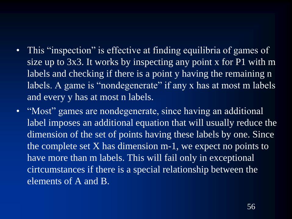
• This “inspection” is effective at finding equilibria of games of
size up to 3x3. It works by inspecting any point x for P1 with m
labels and checking if there is a point y having the remaining n
labels. A game is “nondegenerate” if any x has at most m labels
and every y has at most n labels.
• “Most” games are nondegenerate, since having an additional
label imposes an additional equation that will usually reduce the
dimension of the set of points having these labels by one. Since
the complete set X has dimension m-1, we expect no points to
have more than m labels. This will fail only in exceptional
cirtcumstances if there is a special relationship between the
elements of A and B.

57
n-player general-sum games
• For n-player games with n >= 3, the problem of computing an
NE can no longer be expressed as an LCP. While it can be
expressed as a nonlinear complementarity problem, such
problems are often hopelessly impractical to solve exactly.
• Can solve sequence of LCPs (generalization of Newton’s
method).
– Not globally convergent
• Formulate as constrained optimization (minimization of a
function), but also not globally convergent (e.g., hill climbing,
simulated annealing can get stuck in local optimum)
• Simplicial subdivision algorithm (Scarf)
– Divide space into small regions and search separately over the regions.
• Homotopy method (Govindan and Wilson)

58
Coming up
• Algorithms for computing solution concepts in
strategic-form and extensive-form games, Gambit and
Game Theory Explorer software packages.
• Go through more specific examples of solving linear
programs and linear complementarity programs.
• Solving games with >= 3 players.
• Computing maxmin and minmax for two-player
general-sum games.
• Identifying dominated strategies
– Domination by pure strategies, domination by mixed
strategies, iterated dominance

59
Assignment
• Reading for next class: Game Theory Explorer document and
slides, http://www.cs.cmu.edu/~sganzfri/SeniorThesis.pdf