![Seasonal dynamics of spectral vegetation indices at leaf ... · Leaf level: Norway spruce [-] /g] [-] /g] Date of 2017 Top canopy Low canopy • PRI (and CCI) showed clearly seasonal](https://static.fdocuments.us/doc/165x107/5f132e7f65f3fa1b0213dea8/seasonal-dynamics-of-spectral-vegetation-indices-at-leaf-leaf-level-norway.jpg)
Canopy spectral invariants for remote sensing and model...
17
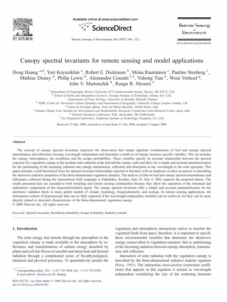
Canopy spectral invariants for remote sensing and model applications Dong Huang a, ⁎ , Yuri Knyazikhin a , Robert E. Dickinson b , Miina Rautiainen c , Pauline Stenberg c , Mathias Disney d , Philip Lewis d , Alessandro Cescatti e,f , Yuhong Tian b , Wout Verhoef g , John V. Martonchik h , Ranga B. Myneni a a Department of Geography, Boston University, 675 Commonwealth Avenue, Boston, MA 02215, USA b School of Earth and Atmospheric Sciences, Georgia Institute of Technology, Atlanta, GA, USA c Department of Forest Ecology, University of Helsinki, Helsinki, Finland d NERC Centre for Terrestrial Carbon Dynamics and Department of Geography, University College London, London, UK e Centro di Ecologia Alpina, Viote del Monte Bondone, 38100 Trento, Italy f Climate Change Unit, Institute for Environment and Sustainability, European Commission Joint Research Centre, Ispra, Italy g National Aerospace Laboratory NLR, Amsterdam, The Netherlands h Jet Propulsion Laboratory, California Institute of Technology, Pasadena, CA, USA Received 15 May 2006; received in revised form 31 July 2006; accepted 2 August 2006 Abstract The concept of canopy spectral invariants expresses the observation that simple algebraic combinations of leaf and canopy spectral transmittance and reflectance become wavelength independent and determine a small set of canopy structure specific variables. This set includes the canopy interceptance, the recollision and the escape probabilities. These variables specify an accurate relationship between the spectral response of a vegetation canopy to the incident solar radiation at the leaf and the canopy scale and allow for a simple and accurate parameterization for the partitioning of the incoming radiation into canopy transmission, reflection and absorption at any wavelength in the solar spectrum. This paper presents a solid theoretical basis for spectral invariant relationships reported in literature with an emphasis on their accuracies in describing the shortwave radiative properties of the three-dimensional vegetation canopies. The analysis of data on leaf and canopy spectral transmittance and reflectance collected during the international field campaign in Flakaliden, Sweden, June 25–July 4, 2002 supports the proposed theory. The results presented here are essential to both modeling and remote sensing communities because they allow the separation of the structural and radiometric components of the measured/modeled signal. The canopy spectral invariants offer a simple and accurate parameterization for the shortwave radiation block in many global models of climate, hydrology, biogeochemistry, and ecology. In remote sensing applications, the information content of hyperspectral data can be fully exploited if the wavelength-independent variables can be retrieved, for they can be more directly related to structural characteristics of the three-dimensional vegetation canopy. © 2006 Elsevier Inc. All rights reserved. Keywords: Spectral invariants; Recollision probability; Escape probability; Radiative transfer 1. Introduction The solar energy that transits through the atmosphere to the vegetation canopy is made available to the atmosphere by re- flectance and transformation of radiant energy absorbed by plants and soil into fluxes of sensible and latent heat and thermal radiation through a complicated series of bio-physiological, chemical and physical processes. To quantitatively predict the vegetation and atmospheric interactions and/or to monitor the vegetated Earth from space, therefore, it is important to specify those environmental variables that determine the shortwave energy conservation in vegetation canopies; that is, partitioning of the incoming radiation between canopy absorption, transmis- sion and reflection. Interaction of solar radiation with the vegetation canopy is described by the three-dimensional radiative transfer equation (Ross, 1981). The interaction cross-section (extinction coeffi- cient) that appears in this equation is treated as wavelength independent considering the size of the scattering elements Remote Sensing of Environment 106 (2007) 106 – 122 www.elsevier.com/locate/rse ⁎ Corresponding author. Tel.: +1 617 353 8846; fax: +1 617 353 8399. E-mail address: [email protected] (D. Huang). 0034-4257/$ - see front matter © 2006 Elsevier Inc. All rights reserved. doi:10.1016/j.rse.2006.08.001
Transcript of Canopy spectral invariants for remote sensing and model...
t 106 (2007) 106–122www.elsevier.com/locate/rse
Remote Sensing of Environmen
Canopy spectral invariants for remote sensing and model applications
Dong Huang a,⁎, Yuri Knyazikhin a, Robert E. Dickinson b, Miina Rautiainen c, Pauline Stenberg c,Mathias Disney d, Philip Lewis d, Alessandro Cescatti e,f, Yuhong Tian b, Wout Verhoef g,
John V. Martonchik h, Ranga B. Myneni a
a Department of Geography, Boston University, 675 Commonwealth Avenue, Boston, MA 02215, USAb School of Earth and Atmospheric Sciences, Georgia Institute of Technology, Atlanta, GA, USA
c Department of Forest Ecology, University of Helsinki, Helsinki, Finlandd NERC Centre for Terrestrial Carbon Dynamics and Department of Geography, University College London, London, UK
e Centro di Ecologia Alpina, Viote del Monte Bondone, 38100 Trento, Italyf Climate Change Unit, Institute for Environment and Sustainability, European Commission Joint Research Centre, Ispra, Italy
g National Aerospace Laboratory NLR, Amsterdam, The Netherlandsh Jet Propulsion Laboratory, California Institute of Technology, Pasadena, CA, USA
Received 15 May 2006; received in revised form 31 July 2006; accepted 2 August 2006
Abstract
The concept of canopy spectral invariants expresses the observation that simple algebraic combinations of leaf and canopy spectraltransmittance and reflectance become wavelength independent and determine a small set of canopy structure specific variables. This set includesthe canopy interceptance, the recollision and the escape probabilities. These variables specify an accurate relationship between the spectralresponse of a vegetation canopy to the incident solar radiation at the leaf and the canopy scale and allow for a simple and accurate parameterizationfor the partitioning of the incoming radiation into canopy transmission, reflection and absorption at any wavelength in the solar spectrum. Thispaper presents a solid theoretical basis for spectral invariant relationships reported in literature with an emphasis on their accuracies in describingthe shortwave radiative properties of the three-dimensional vegetation canopies. The analysis of data on leaf and canopy spectral transmittance andreflectance collected during the international field campaign in Flakaliden, Sweden, June 25–July 4, 2002 supports the proposed theory. Theresults presented here are essential to both modeling and remote sensing communities because they allow the separation of the structural andradiometric components of the measured/modeled signal. The canopy spectral invariants offer a simple and accurate parameterization for theshortwave radiation block in many global models of climate, hydrology, biogeochemistry, and ecology. In remote sensing applications, theinformation content of hyperspectral data can be fully exploited if the wavelength-independent variables can be retrieved, for they can be moredirectly related to structural characteristics of the three-dimensional vegetation canopy.© 2006 Elsevier Inc. All rights reserved.
Keywords: Spectral invariants; Recollision probability; Escape probability; Radiative transfer
1. Introduction
The solar energy that transits through the atmosphere to thevegetation canopy is made available to the atmosphere by re-flectance and transformation of radiant energy absorbed byplants and soil into fluxes of sensible and latent heat and thermalradiation through a complicated series of bio-physiological,chemical and physical processes. To quantitatively predict the
⁎ Corresponding author. Tel.: +1 617 353 8846; fax: +1 617 353 8399.E-mail address: [email protected] (D. Huang).
0034-4257/$ - see front matter © 2006 Elsevier Inc. All rights reserved.doi:10.1016/j.rse.2006.08.001
vegetation and atmospheric interactions and/or to monitor thevegetated Earth from space, therefore, it is important to specifythose environmental variables that determine the shortwaveenergy conservation in vegetation canopies; that is, partitioningof the incoming radiation between canopy absorption, transmis-sion and reflection.
Interaction of solar radiation with the vegetation canopy isdescribed by the three-dimensional radiative transfer equation(Ross, 1981). The interaction cross-section (extinction coeffi-cient) that appears in this equation is treated as wavelengthindependent considering the size of the scattering elements
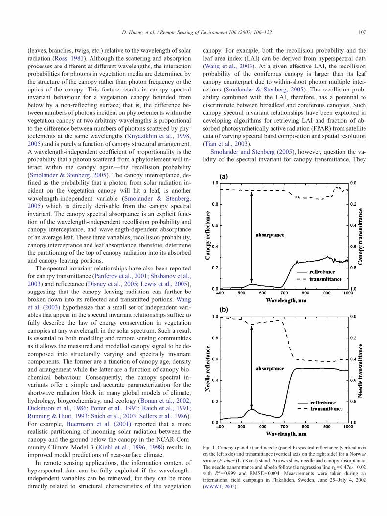
Fig. 1. Canopy (panel a) and needle (panel b) spectral reflectance (vertical axison the left side) and transmittance (vertical axis on the right side) for a Norwayspruce (P. abies (L.) Karst) stand. Arrows show needle and canopy absorptance.The needle transmittance and albedo follow the regression line τL=0.47ω−0.02with R2=0.999 and RMSE=0.004. Measurements were taken during aninternational field campaign in Flakaliden, Sweden, June 25–July 4, 2002(WWW1, 2002).
107D. Huang et al. / Remote Sensing of Environment 106 (2007) 106–122
(leaves, branches, twigs, etc.) relative to the wavelength of solarradiation (Ross, 1981). Although the scattering and absorptionprocesses are different at different wavelengths, the interactionprobabilities for photons in vegetation media are determined bythe structure of the canopy rather than photon frequency or theoptics of the canopy. This feature results in canopy spectralinvariant behaviour for a vegetation canopy bounded frombelow by a non-reflecting surface; that is, the difference be-tween numbers of photons incident on phytoelements within thevegetation canopy at two arbitrary wavelengths is proportionalto the difference between numbers of photons scattered by phy-toelements at the same wavelengths (Knyazikhin et al., 1998,2005) and is purely a function of canopy structural arrangement.A wavelength-independent coefficient of proportionality is theprobability that a photon scattered from a phytoelement will in-teract within the canopy again—the recollision probability(Smolander & Stenberg, 2005). The canopy interceptance, de-fined as the probability that a photon from solar radiation in-cident on the vegetation canopy will hit a leaf, is anotherwavelength-independent variable (Smolander & Stenberg,2005) which is directly derivable from the canopy spectralinvariant. The canopy spectral absorptance is an explicit func-tion of the wavelength-independent recollision probability andcanopy interceptance, and wavelength-dependent absorptanceof an average leaf. These three variables, recollision probability,canopy interceptance and leaf absorptance, therefore, determinethe partitioning of the top of canopy radiation into its absorbedand canopy leaving portions.
The spectral invariant relationships have also been reportedfor canopy transmittance (Panferov et al., 2001; Shabanov et al.,2003) and reflectance (Disney et al., 2005; Lewis et al., 2005),suggesting that the canopy leaving radiation can further bebroken down into its reflected and transmitted portions. Wanget al. (2003) hypothesize that a small set of independent vari-ables that appear in the spectral invariant relationships suffice tofully describe the law of energy conservation in vegetationcanopies at any wavelength in the solar spectrum. Such a resultis essential to both modeling and remote sensing communitiesas it allows the measured and modelled canopy signal to be de-composed into structurally varying and spectrally invariantcomponents. The former are a function of canopy age, densityand arrangement while the latter are a function of canopy bio-chemical behaviour. Consequently, the canopy spectral in-variants offer a simple and accurate parameterization for theshortwave radiation block in many global models of climate,hydrology, biogeochemistry, and ecology (Bonan et al., 2002;Dickinson et al., 1986; Potter et al., 1993; Raich et al., 1991;Running & Hunt, 1993; Saich et al., 2003; Sellers et al., 1986).For example, Buermann et al. (2001) reported that a morerealistic partitioning of incoming solar radiation between thecanopy and the ground below the canopy in the NCAR Com-munity Climate Model 3 (Kiehl et al., 1996, 1998) results inimproved model predictions of near-surface climate.
In remote sensing applications, the information content ofhyperspectral data can be fully exploited if the wavelength-independent variables can be retrieved, for they can be moredirectly related to structural characteristics of the vegetation
canopy. For example, both the recollision probability and theleaf area index (LAI) can be derived from hyperspectral data(Wang et al., 2003). At a given effective LAI, the recollisionprobability of the coniferous canopy is larger than its leafcanopy counterpart due to within-shoot photon multiple inter-actions (Smolander & Stenberg, 2005). The recollision prob-ability combined with the LAI, therefore, has a potential todiscriminate between broadleaf and coniferous canopies. Suchcanopy spectral invariant relationships have been exploited indeveloping algorithms for retrieving LAI and fraction of ab-sorbed photosynthetically active radiation (FPAR) from satellitedata of varying spectral band composition and spatial resolution(Tian et al., 2003).
Smolander and Stenberg (2005), however, question the va-lidity of the spectral invariant for canopy transmittance. They
108 D. Huang et al. / Remote Sensing of Environment 106 (2007) 106–122
show that while the recollision probability and canopy inter-ceptance perform well in estimating the spectral absorption ofboth homogeneous leaf and shoot canopies, a proposed struc-tural parameter for separation of downward portion of the can-opy leaving radiation (Knyazikhin et al., 1998; Panferov et al.,2001; Shabanov et al., 2003) can fail to predict spectral trans-mittance of the coniferous canopy and spectral transmittance ofthe leaf canopy at high LAI values. Panferov et al. (2001)suggest that the spectral invariant relationship is not valid forcanopy reflectance while Lewis et al. (2003, 2005) and Disneyet al. (2005) have demonstrated its validity to describe thetransformation for leaf absorptance spectrum to canopy spectralreflectance. The lack of physically based definitions ofwavelength-independent variables that determine separation ofthe down- and upward portions of the canopy leaving radiationis responsible for these conflicting results (Smolander &Stenberg, 2005). The aim of the present paper is to provide asolid theoretical basis for canopy spectral invariants. Morespecifically, it addresses the following three questions. (i) Howcan the wavelength-independent structural parameters be de-fined to achieve an accurate and consistent parameterizationfor canopy spectral response to the incident solar radiation?(ii) How is the recollision probability related to the wavelength-independent variables that control up- and downward portionsof the canopy leaving radiation? Finally, (iii) How accurate arethese spectral invariant relationships?
The paper is organized as follows. Canopy spectral invariantrelationships reported in the literature are analyzed with datafrom an international field campaign in a coniferous forest nearFlakaliden, Sweden, in Section 2 and Appendix A. Expansionof the 3D radiation field in the successive order of scattering, orNeumann series, and its properties are discussed in Section 3and Appendix B. Spectral invariants for canopy interactioncoefficients, reflectance, transmittance and bidirectional reflec-tance factors and their accuracies are studied in Sections 4–6.Simplified spectral invariant relationships for use in remotesensing and model studies are analyzed in Section 7. Finally,Section 8 summarizes the results.
2. Canopy spectral invariants: observations
The aim of this section is to illustrate the canopy spectralinvariant relationships reported in the literature and to introducetheir basic properties using field data collected during aninternational field campaign in Flakaliden, Sweden, June 25–July 4, 2002. A description of instrumentation, measurementapproach and data processing is given in Appendix A.1. Itshould be noted that the spectral invariant is formulated for avegetation canopy bounded from below by a non-reflectingsurface. However, we will use measured spectra without cor-recting for canopy substrate effects (i.e., the fact that observedcanopies do not have totally absorbing lower boundaries). Theimpact of surface reflection on canopy reflectance, absorptanceand transmittance is discussed in Appendix A.2 and summa-rized in Fig. A1.
The canopy transmittance (reflectance) is the ratio of themean downward radiation flux density at the canopy bottom
(mean upward radiation flux density at the canopy top) to thedownward radiation flux density above the canopy. Similarly,canopy absorptance is the portion of radiation incident on thevegetation canopy that the canopy absorbs. These variables arethe three basic components of the law of shortwave energyconservation which describe canopy spectral response to inci-dent solar radiation at the canopy scale. If reflectance of theground below the vegetation is zero, the portion of radiationabsorbed, a(λ), transmitted, t(λ), or reflected, r(λ), by the can-opy is unity, i.e.,
tðkÞ þ rðkÞ þ aðkÞ ¼ 1: ð1Þ
Fig. 1a shows canopy transmittance and reflectance spectraof a 50 m×50 m plot with planted 40-year-old Norway spruce(Appendix A.1). This plot had been subjected to irrigation andfertilization since 1987. The effective LAI is 4.37.
The leaf transmittance (reflectance) is the portion of radiationflux density incident on the leaf surface that the leaf transmits(reflects). These variables characterize the canopy spectral be-havior at the leaf scale, are determined by the leaf biochemicalconstituents, and can vary with tree species, growth conditions,leaf age and their location in the canopy space. The leaf albedo,ω(λ), is the sum of the leaf reflectance, ρL(λ), and transmittance,τL(λ), i.e.,
xðkÞ ¼ qLðkÞ þ sLðkÞ: ð2Þ
Fig. 1b shows spectral transmittance and reflectance of anaverage needle derived from the Flakaliden data (Appendix A.1).Measured spectra shown in Fig. 1a and b are used in ourexamples.
2.1. Canopy spectral invariant for interaction coefficient
The canopy interaction coefficient, i(λ), is the ratio of thecanopy absorptance a(λ) to the absorptance 1−ω(λ) of anaverage leaf (Knyazikhin et al., 2005, p. 633), i.e.,
i kð Þ ¼ aðkÞ1−xðkÞ ¼
1−tðkÞ−rðkÞ1−xðkÞ : ð3Þ
For a vegetation canopy bounded at its bottom by a blacksurface, this variable is the mean number of photon interactionswith phytoelements at wavelength λ. The portion of photonsscattered by leaves is ω(λ)i(λ). If ω(λ)=0, the canopy inter-action coefficient, i0, is the probability that a photon from theincident radiation will hit a phytoelement—the canopy inter-ceptance (Smolander & Stenberg, 2005). For a vegetation can-opy with non-reflecting leaves, the canopy absorptance andinterceptance coincide.
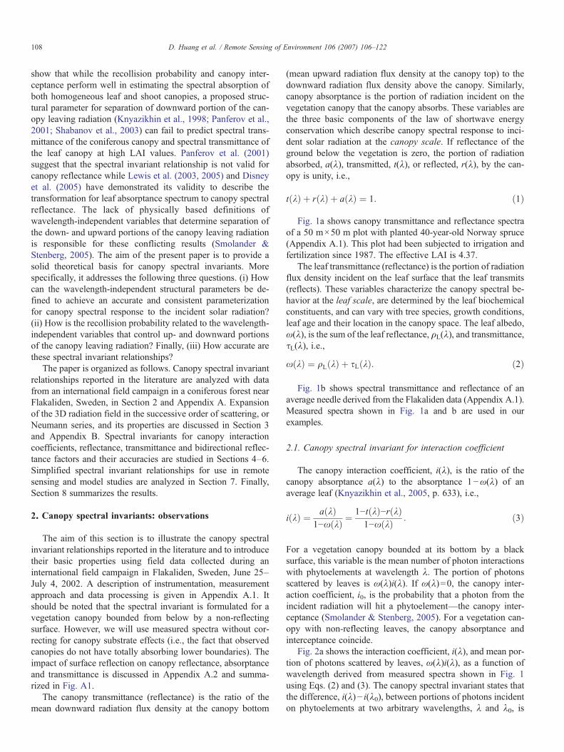
Fig. 2a shows the interaction coefficient, i(λ), and mean por-tion of photons scattered by leaves, ω(λ)i(λ), as a function ofwavelength derived from measured spectra shown in Fig. 1using Eqs. (2) and (3). The canopy spectral invariant states thatthe difference, i(λ)− i(λ0), between portions of photons incidenton phytoelements at two arbitrary wavelengths, λ and λ0, is
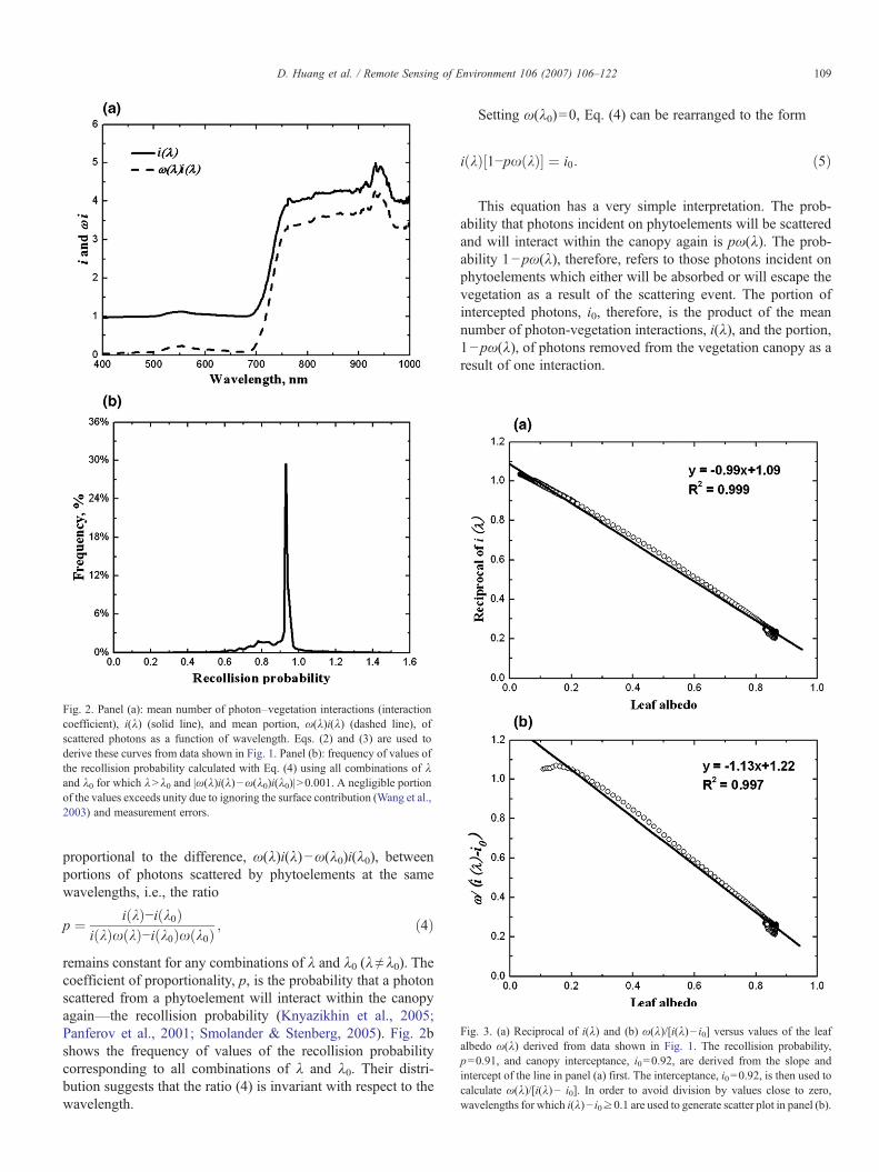
Fig. 2. Panel (a): mean number of photon–vegetation interactions (interactioncoefficient), i(λ) (solid line), and mean portion, ω(λ)i(λ) (dashed line), oscattered photons as a function of wavelength. Eqs. (2) and (3) are used toderive these curves from data shown in Fig. 1. Panel (b): frequency of values othe recollision probability calculated with Eq. (4) using all combinations of λand λ0 for which λNλ0 and |ω(λ)i(λ)−ω(λ0)i(λ0)|N0.001. A negligible portionof the values exceeds unity due to ignoring the surface contribution (Wang et al.2003) and measurement errors.
109D. Huang et al. / Remote Sensing of Environment 106 (2007) 106–122
f
f
,
Fig. 3. (a) Reciprocal of i(λ) and (b) ω(λ)/[i(λ)− i0] versus values of the leafalbedo ω(λ) derived from data shown in Fig. 1. The recollision probability,p=0.91, and canopy interceptance, i0=0.92, are derived from the slope andintercept of the line in panel (a) first. The interceptance, i0=0.92, is then used tocalculate ω(λ)/[i(λ)− i0]. In order to avoid division by values close to zero,wavelengths for which i(λ)− i0≥0.1 are used to generate scatter plot in panel (b).
proportional to the difference, ω(λ)i(λ)−ω(λ0)i(λ0), betweenportions of photons scattered by phytoelements at the samewavelengths, i.e., the ratio
p ¼ iðkÞ−iðk0ÞiðkÞxðkÞ−iðk0Þxðk0Þ ; ð4Þ
remains constant for any combinations of λ and λ0 (λ≠λ0). Thecoefficient of proportionality, p, is the probability that a photonscattered from a phytoelement will interact within the canopyagain—the recollision probability (Knyazikhin et al., 2005;Panferov et al., 2001; Smolander & Stenberg, 2005). Fig. 2bshows the frequency of values of the recollision probabilitycorresponding to all combinations of λ and λ0. Their distri-bution suggests that the ratio (4) is invariant with respect to thewavelength.
Setting ω(λ0)=0, Eq. (4) can be rearranged to the form
iðkÞ½1−pxðkÞ� ¼ i0: ð5Þ
This equation has a very simple interpretation. The prob-ability that photons incident on phytoelements will be scatteredand will interact within the canopy again is pω(λ). The prob-ability 1−pω(λ), therefore, refers to those photons incident onphytoelements which either will be absorbed or will escape thevegetation as a result of the scattering event. The portion ofintercepted photons, i0, therefore, is the product of the meannumber of photon-vegetation interactions, i(λ), and the portion,1−pω(λ), of photons removed from the vegetation canopy as aresult of one interaction.
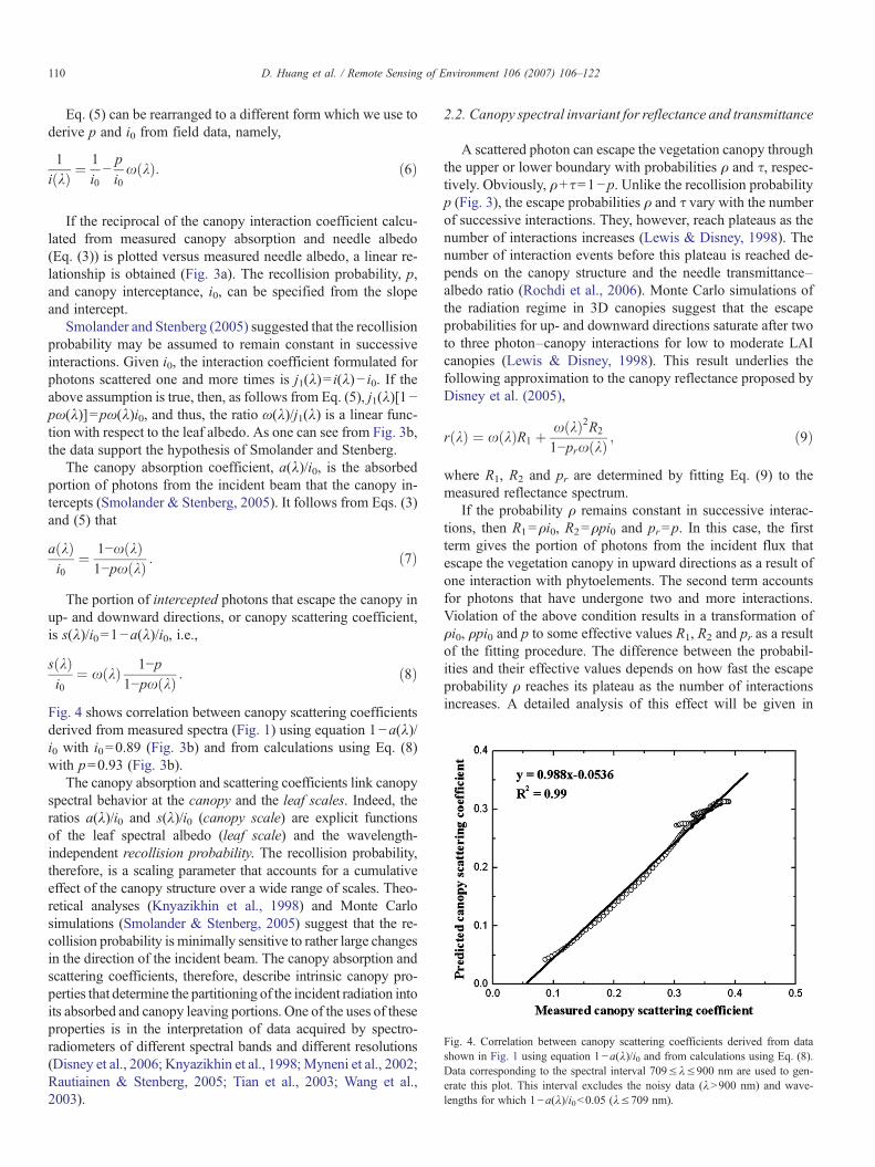
Fig. 4. Correlation between canopy scattering coefficients derived from datashown in Fig. 1 using equation 1−a(λ)/i0 and from calculations using Eq. (8).Data corresponding to the spectral interval 709≤λ≤900 nm are used to gen-erate this plot. This interval excludes the noisy data (λN900 nm) and wave-lengths for which 1−a(λ)/i0b0.05 (λ≤709 nm).
110 D. Huang et al. / Remote Sensing of Environment 106 (2007) 106–122
Eq. (5) can be rearranged to a different form which we use toderive p and i0 from field data, namely,
1iðkÞ ¼
1i0−pi0x kð Þ: ð6Þ
If the reciprocal of the canopy interaction coefficient calcu-lated from measured canopy absorption and needle albedo(Eq. (3)) is plotted versus measured needle albedo, a linear re-lationship is obtained (Fig. 3a). The recollision probability, p,and canopy interceptance, i0, can be specified from the slopeand intercept.
Smolander and Stenberg (2005) suggested that the recollisionprobability may be assumed to remain constant in successiveinteractions. Given i0, the interaction coefficient formulated forphotons scattered one and more times is j1(λ)= i(λ)− i0. If theabove assumption is true, then, as follows from Eq. (5), j1(λ)[1−pω(λ)]=pω(λ)i0, and thus, the ratio ω(λ)/j1(λ) is a linear func-tion with respect to the leaf albedo. As one can see from Fig. 3b,the data support the hypothesis of Smolander and Stenberg.
The canopy absorption coefficient, a(λ)/i0, is the absorbedportion of photons from the incident beam that the canopy in-tercepts (Smolander & Stenberg, 2005). It follows from Eqs. (3)and (5) that
aðkÞi0
¼ 1−xðkÞ1−pxðkÞ : ð7Þ
The portion of intercepted photons that escape the canopy inup- and downward directions, or canopy scattering coefficient,is s(λ)/i0=1−a(λ)/i0, i.e.,
sðkÞi0
¼ x kð Þ 1−p1−pxðkÞ : ð8Þ
Fig. 4 shows correlation between canopy scattering coefficientsderived from measured spectra (Fig. 1) using equation 1−a(λ)/i0 with i0=0.89 (Fig. 3b) and from calculations using Eq. (8)with p=0.93 (Fig. 3b).
The canopy absorption and scattering coefficients link canopyspectral behavior at the canopy and the leaf scales. Indeed, theratios a(λ)/i0 and s(λ)/i0 (canopy scale) are explicit functionsof the leaf spectral albedo (leaf scale) and the wavelength-independent recollision probability. The recollision probability,therefore, is a scaling parameter that accounts for a cumulativeeffect of the canopy structure over a wide range of scales. Theo-retical analyses (Knyazikhin et al., 1998) and Monte Carlosimulations (Smolander & Stenberg, 2005) suggest that the re-collision probability is minimally sensitive to rather large changesin the direction of the incident beam. The canopy absorption andscattering coefficients, therefore, describe intrinsic canopy pro-perties that determine the partitioning of the incident radiation intoits absorbed and canopy leaving portions. One of the uses of theseproperties is in the interpretation of data acquired by spectro-radiometers of different spectral bands and different resolutions(Disney et al., 2006; Knyazikhin et al., 1998; Myneni et al., 2002;Rautiainen & Stenberg, 2005; Tian et al., 2003; Wang et al.,2003).
2.2. Canopy spectral invariant for reflectance and transmittance
A scattered photon can escape the vegetation canopy throughthe upper or lower boundary with probabilities ρ and τ, respec-tively. Obviously, ρ+τ=1−p. Unlike the recollision probabilityp (Fig. 3), the escape probabilities ρ and τ vary with the numberof successive interactions. They, however, reach plateaus as thenumber of interactions increases (Lewis & Disney, 1998). Thenumber of interaction events before this plateau is reached de-pends on the canopy structure and the needle transmittance–albedo ratio (Rochdi et al., 2006). Monte Carlo simulations ofthe radiation regime in 3D canopies suggest that the escapeprobabilities for up- and downward directions saturate after twoto three photon–canopy interactions for low to moderate LAIcanopies (Lewis & Disney, 1998). This result underlies thefollowing approximation to the canopy reflectance proposed byDisney et al. (2005),
r kð Þ ¼ x kð ÞR1 þ xðkÞ2R2
1−prxðkÞ ; ð9Þ
where R1, R2 and pr are determined by fitting Eq. (9) to themeasured reflectance spectrum.
If the probability ρ remains constant in successive interac-tions, then R1=ρi0, R2=ρpi0 and pr=p. In this case, the firstterm gives the portion of photons from the incident flux thatescape the vegetation canopy in upward directions as a result ofone interaction with phytoelements. The second term accountsfor photons that have undergone two and more interactions.Violation of the above condition results in a transformation ofρi0, ρpi0 and p to some effective values R1, R2 and pr as a resultof the fitting procedure. The difference between the probabil-ities and their effective values depends on how fast the escapeprobability ρ reaches its plateau as the number of interactionsincreases. A detailed analysis of this effect will be given in
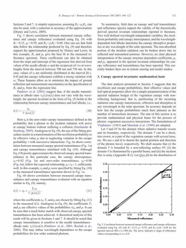
Fig. 5. Correlation between measured canopy reflectance and canopy reflectanceevaluated using Eq. (9) with R1=0.15, pr=0.59, and R2=prR1=0.09 for thespectral interval 400≤λ≤900 nm. The arrow indicates a range of reflectancevalues corresponding to ω≥0.9.
111D. Huang et al. / Remote Sensing of Environment 106 (2007) 106–122
Sections 5 and 7. A simpler expression, assuming R2=prR1, canalso be used, with a reduction in accuracy of the approximation(Disney and Lewis, 2005).
Fig. 5 shows correlation between measured canopy reflec-tance and canopy reflectance evaluated using Eq. (9) withR1=0.15, pr=0.59, and R2=prR1=0.09. One can see that fielddata follow the relationship predicted by Eq. (9) and thereforesupport the approximation proposed by Disney and Lewis. Inthis example, R1 and pr give the best fit to the measured re-flectance spectrum. These coefficients can also be obtainedfrom the slope and intercept of the regression line derived fromvalues of the needle albedo ω and the reciprocal of r/ω at wave-lengths from the interval between 700 nm and 750 nm. In thiscase, values of ω are uniformly distributed in the interval [0.1,0.9] and the canopy reflectance exhibits a strong variation withω. These features allow us to minimize the impact of groundreflection and measurement uncertainties on the specification ofR1 and pr from the regression line.
Panferov et al. (2001) suggest that, if the needle transmit-tance to albedo ratio τL(λ)/ω(λ) does not vary with the wave-length, the spectral invariant in the form of Eq. (5) holds in therelationship between canopy transmittance and leaf albedo, i.e.,
t kð Þ ¼ t01−ptxðkÞ : ð10Þ
Here t0 is the zero-order canopy transmittance defined as theprobability that a photon in the incident radiation will arriveat canopy bottom without suffering a collision (Smolander &Stenberg, 2005). Analogous to Eq. (9), the use of the fitting pro-cedure results in a transformation of the recollision probability toits effective value pt due to neglecting variation in the escapeprobability τ with successive interactions. Fig. 6a shows corre-lation between measured canopy spectral transmittance (Fig. 1a)and canopy transmittance simulated with Eq. (10). AlthoughEq. (10) poorly approximates the observed canopy spectral trans-mittance in this particular case, the canopy interceptance,i0=0.92 (Fig. 3a) and zero-order transmittance, t0=0.06(Fig. 6a), follow the expected relationship, t0+ i0=1, sufficientlywell. In this example, t0 and pt were specified by fitting Eq. (10)to the measured transmittance spectrum shown in Fig. 1a.
Fig. 6b shows correlation between measured canopy trans-mittance and canopy transmittance evaluated with an equationsimilar to Eq. (9), namely,
t kð Þ ¼ t0 þ T1x1−ptxðkÞ ; ð11Þ
where the coefficients t0, T1 and pt are chosen by fitting Eq. (11)to the measured t(λ). Analogous to Eq. (9), the coefficients T1and pt are effective values of the probabilities τi0, and p. It canbe seen that a much better match with observed canopy spectraltransmittances has been achieved. A theoretical analysis of thisresult will be given in Sections 5 and 7. It should be noted thatcanopy transmittance is sensitive to the needle transmittance–albedo ratio τL(λ)/ω(λ) (Panferov et al., 2001; Rochdi et al.,2006). This may imbue wavelength dependence to the escapeprobabilities for low order scattered photons.
To summarize, field data on canopy and leaf transmittanceand reflectance spectra support the validity of the theoreticallyderived spectral invariant relationships reported in literature.Two well-defined wavelength-independent variables, the recol-lision probability and canopy interceptance, and the wavelength-dependent leaf albedo determine the canopy absorptive proper-ties at any wavelength of the solar spectrum. The non-absorbedportion of the incident radiation can be broken down into itsreflected and transmitted portions. However, no clear physicalinterpretation of the canopy structure dependent coefficients, prand pt, appeared in the spectral invariant relationships for can-opy reflectance and transmittance has been reported. This cur-rently hinders their use in remote sensing and model studies.
3. Canopy spectral invariants: mathematical basis
The data analysis presented in Section 2 suggests that therecollision and escape probabilities, their effective values andleaf optical properties allow for a simple parameterization of thespectral radiation budget of the vegetation canopy with non-reflecting background; that is, partitioning of the incomingradiation into canopy transmission, reflection and absorption atany wavelength in the solar spectrum. Its accuracy depends onhow fast the escape probabilities reach their plateaus as thenumber of interactions increases. The aim of this section is toprovide mathematical and physical bases for the process ofphoton–vegetation successive interactions. The formulations ofVladimirov (1963) and Marchuk et al. (1980) are adopted.
Let V and δV be the domain where radiative transfer occursand its boundary, respectively. The domain V can be a shoot,tree crown, or a part of the vegetation canopy with several trees,etc. We use x and Ω to denote the spatial position and directionof the photon travel, respectively. We shall assume that (i) thedomain V is bounded by a non-reflecting surface δV; (ii) thedomain V is illuminated by a parallel beam; and (iii) the incidentflux is unity (Appendix B.2). Let Q0(x,Ω) be the distribution of
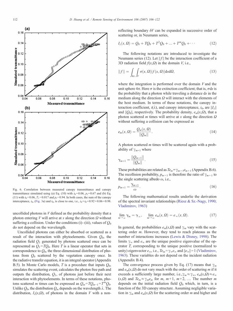
Fig. 6. Correlation between measured canopy transmittance and canopytransmittance simulated using (a) Eq. (10) with t0=0.06, pt=0.67 and (b) Eq.(11) with t0=0.06, T1=0.017 and pt=0.94. In both cases, the sum of the canopyinterceptance, i0, (Fig. 3a) and t0, is close to one, i.e., i0+ t0=0.92+0.06=0.98.
112 D. Huang et al. / Remote Sensing of Environment 106 (2007) 106–122
uncollided photons in V defined as the probability density that aphoton entering V will arrive at x along the direction Ω withoutsuffering a collision. Under the conditions (i)–(iii), values of Q0
do not depend on the wavelength.Uncollided photons can either be absorbed or scattered as a
result of the interaction with phytoelements. Given Q0, theradiation field Q1 generated by photons scattered once can berepresented as Q1=TQ0. Here T is a linear operator that sets incorrespondence to Q0, the three-dimensional distribution of pho-tons from Q0 scattered by the vegetation canopy once. Inthe radiative transfer equation, it is an integral operator (AppendixB.5). In Monte Carlo models, T is a procedure that inputs Q0,simulates the scattering event, calculates the photon free path andoutputs the distribution, Q1, of photons just before their nextinteraction with phytoelements. In terms of these notations, pho-tons scattered m times can be expressed as Qm=TQm−1=T
mQ0.UnlikeQ0, the distributionQm depends on the wavelength λ. Thedistribution, Iλ(x,Ω), of photons in the domain V with a non-
reflecting boundary δV can be expanded in successive order ofscattering or, in Neumann series,
Ikðx;XÞ ¼ Q0 þ TQ0 þ T2Q0 þ …þ TmQ0 þ : : : ð12Þ
The following notations are introduced to investigate theNeumann series (12). Let || f || be the interaction coefficient of a3D radiation field f (x,Ω) in the domain V, i.e.,
jj f jj ¼Z4p
ZV
rðx;XÞj f ðx;XÞjdxdX; ð13Þ
where the integration is performed over the domain V and theunit sphere 4π. Here σ is the extinction coefficient; that is, σds isthe probability that a photon while traveling a distance ds in themedium along the direction Ω will interact with the elements ofthe host medium. In terms of these notations, the canopy in-teraction coefficient, i(λ), and canopy interceptance, i0, are ||Iλ||and ||Q0||, respectively. The probability density, em(x,Ω), that aphoton scattered m times will arrive at x along the direction Ωwithout suffering a collision can be expressed as
em x;Xð Þ ¼ Qmðx;XÞjjQmjj : ð14Þ
A photon scattered m times will be scattered again with a prob-ability of γm+1 where
gmþ1 ¼jjQmþ1jjjjQmjj : ð15Þ
These probabilities are related asTem=γm+1em+1 (Appendix B.6).The recollision probability, pm+1 is therefore the ratio of γm+1 tothe single scattering albedo ω, i.e.,
pmþ1 ¼ gmþ1
x: ð16Þ
The following mathematical results underlie the derivationof the spectral invariant relationships (Riesz & Sz.-Nagy, 1990;Vladimirov, 1963)
limmYl
gm ¼ gl; limmYl
emðx;XÞ ¼ elðx;XÞ: ð17Þ
In general, the probabilities em(x,Ω) and γm vary with the scat-tering order m. However, they tend to reach plateaus as thenumber of interactions increases (Lewis & Disney, 1998). Thelimits γ∞ and e∞ are the unique positive eigenvalue of the op-erator T, corresponding to the unique positive (normalized tounity) eigenvector e∞, i.e., Tem=γ∞e∞ and ||e∞|| =1 (Vladimirov,1963). These variables do not depend on the incident radiation(Appendix B.4).
The convergence process given by Eq. (17) means that γmand em(x,Ω) do not vary much with the order of scattering m if itexceeds a sufficiently large number, i.e.,γm≈γ∞, em(x,Ω)≈e∞(x,Ω) and Tem≈γmem for m, m+1, m+2, …. The number mdepends on the initial radiation field Q0 which, in turn, is afunction of the 3D canopy structure. Assuming negligible varia-tion in γm and em(x,Ω) for the scattering order m and higher and
113D. Huang et al. / Remote Sensing of Environment 106 (2007) 106–122
accounting for Eqs. (12) and (14), the radiation field Iλ(x,Ω) canbe approximated as (Appendix B.6)
Ikðx;XÞ ¼ Ik;mðx;XÞ þ dm; ð18Þ
where
Ik;m x;Xð Þ ¼Xmk¼0
jjQk jjek þ jjQmjj gmþ1
1−gmþ1emþ1; ð19Þ
dm ¼ Ikðx;XÞ−Ik;mðx;XÞ ð20ÞThe radiation field Iλ,m(x,Ω) is the mth approximation to the
3D radiation field in the vegetation canopy, and δm is its error.Note that the non-negativity of ek, k=1,2, …, are critical toderive Eq. (20). Eqs. (18)–(20) underlie the derivation of thecanopy spectral invariant relationships and their accuracies. Itshould be emphasized that these results are not tied to a particularcanopy radiation model. The operator T represents any linearmodel that simulates the scattering event and the photon freepath for photons from a given field. We will use the 3D radiativetransfer equation to specify the operator T (Appendix B.5).
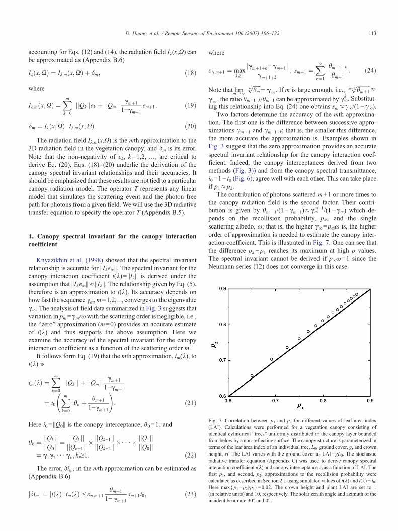
Fig. 7. Correlation between p1 and p2 for different values of leaf area index(LAI). Calculations were performed for a vegetation canopy consisting ofidentical cylindrical “trees” uniformly distributed in the canopy layer boundedfrom below by a non-reflecting surface. The canopy structure is parameterized interms of the leaf area index of an individual tree, L0, ground cover, g, and crownheight, H. The LAI varies with the ground cover as LAI=gL0. The stochasticradiative transfer equation (Appendix C) was used to derive canopy spectralinteraction coefficient i(λ) and canopy interceptance i0 as a function of LAI. Thefirst p1, and second, p2, approximations to the recollision probability werecalculated as described in Section 2.1 using simulated values of i(λ) and i(λ)− i0.Here max{|p1−p2|/p1}=0.02. The crown height and plant LAI are set to 1(in relative units) and 10, respectively. The solar zenith angle and azimuth of theincident beam are 30° and 0°.
4. Canopy spectral invariant for the canopy interactioncoefficient
Knyazikhin et al. (1998) showed that the spectral invariantrelationship is accurate for ||Iλe∞||. The spectral invariant for thecanopy interaction coefficient i(λ)= ||Iλ|| is derived under theassumption that ||Iλe∞||≈ ||Iλ||. The relationship given by Eq. (5),therefore is an approximation to i(λ). Its accuracy depends onhow fast the sequence γm,m=1,2,…, converges to the eigenvalueγ∞. The analysis of field data summarized in Fig. 3 suggests thatvariation in pm=γm/ωwith the scattering order is negligible, i.e.,the “zero” approximation (m=0) provides an accurate estimateof i(λ) and thus supports the above assumption. Here weexamine the accuracy of the spectral invariant for the canopyinteraction coefficient as a function of the scattering order m.
It follows form Eq. (19) that the mth approximation, im(λ), toi(λ) is
im kð Þ ¼Xmk¼0
jjQk jj þ jjQmjj gmþ1
1−gmþ1
¼ i0Xmk¼0
hk þ hmþ1
1−gmþ1
!: ð21Þ
Here i0= ||Q0|| is the canopy interceptance; θ0=1, and
hk ¼ jjQk jjjjQ0jj ¼
jjQk jjjjQk−1jj �
jjQk−1jjjjQk−2jj �
: : : � jjQ1jjjjQ0jj
¼ g1g2 : : : gk ; kz1: ð22ÞThe error, δim, in the mth approximation can be estimated as
(Appendix B.6)
jdimj ¼ ji kð Þ−im kð ÞjV eg;mþ1hmþ1
1− gmþ1smþ1i0; ð23Þ
where
eg;mþ1 ¼ maxkz1
jgmþ1þk− gmþ1jgmþ1þk
; smþ1 ¼Xlk¼1
hmþ1þk
hmþ1: ð24Þ
Note that limmYl
ffiffiffiffiffiffihmm
p ¼ gl. If m is large enough, i.e.,ffiffiffiffiffiffiffiffiffiffihmþ1
mþ1p
c
gl, the ratio θm+1+k/θm+1 can be approximated by γ∞k . Substitut-
ing this relationship into Eq. (24) one obtains sm≈γ∞/(1−γ∞).Two factors determine the accuracy of the mth approxima-
tion. The first one is the difference between successive appro-ximations γm+1 and γm+1+k; that is, the smaller this difference,the more accurate the approximation is. Examples shown inFig. 3 suggest that the zero approximation provides an accuratespectral invariant relationship for the canopy interaction coef-ficient. Indeed, the canopy interceptances derived from twomethods (Fig. 3)) and from the canopy spectral transmittance,i0=1− t0 (Fig. 6), agree well with each other. This can take placeif p1≈p2.
The contribution of photons scattered m+1 or more times tothe canopy radiation field is the second factor. Their contri-bution is given by θm+1/(1−γm+1)≈γ∞
m+1/(1−γ∞) which de-pends on the recollision probability, p∞, and the singlescattering albedo, ω; that is, the higher γ∞=p∞ω is, the higherorder of approximation is needed to estimate the canopy inter-action coefficient. This is illustrated in Fig. 7. One can see thatthe difference p2−p1 reaches its maximum at high p values.The spectral invariant cannot be derived if p∞ω=1 since theNeumann series (12) does not converge in this case.
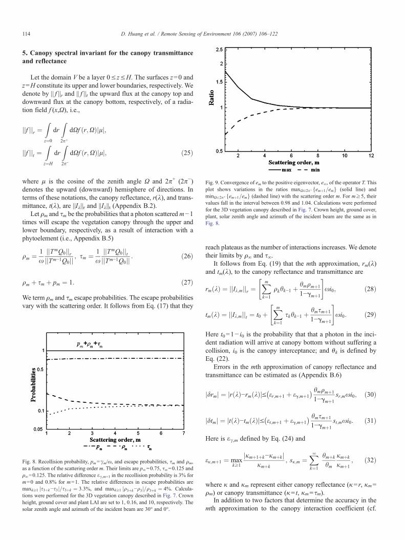
Fig. 9. Convergence of em to the positive eigenvector, e∞, of the operator T. Thisplot shows variations in the ratios maxXa2pþfemþ1=emg (solid line) andminXa2pþfemþ1=emg (dashed line) with the scattering order m. For m≥5, theirvalues fall in the interval between 0.98 and 1.04. Calculations were performedfor the 3D vegetation canopy described in Fig. 7. Crown height, ground cover,plant, solar zenith angle and azimuth of the incident beam are the same as inFig. 8.
114 D. Huang et al. / Remote Sensing of Environment 106 (2007) 106–122
5. Canopy spectral invariant for the canopy transmittanceand reflectance
Let the domain V be a layer 0≤ z≤H. The surfaces z=0 andz=H constitute its upper and lower boundaries, respectively. Wedenote by || f ||r and || f ||t the upward flux at the canopy top anddownward flux at the canopy bottom, respectively, of a radia-tion field f (x,Ω), i.e.,
jjf jjr ¼Zz¼0
drZ2pþ
dXf ðr;XÞjlj;
jjf jjt ¼Zz¼H
drZ2p−
dXf ðr;XÞjlj; ð25Þ
where μ is the cosine of the zenith angle Ω and 2π+ (2π−)denotes the upward (downward) hemisphere of directions. Interms of these notations, the canopy reflectance, r(λ), and trans-mittance, t(λ), are ||Iλ||r and ||Iλ||t (Appendix B.2).
Let ρm and τm be the probabilities that a photon scatteredm−1times will escape the vegetation canopy through the upper andlower boundary, respectively, as a result of interaction with aphytoelement (i.e., Appendix B.5)
qm ¼ 1x
jjTmQ0jjrjjTm−1Q0jj ; sm ¼ 1
xjjTmQ0jjtjjTm−1Q0jj : ð26Þ
qm þ sm þ pm ¼ 1: ð27Þ
We term ρm and τm escape probabilities. The escape probabilitiesvary with the scattering order. It follows from Eq. (17) that they
Fig. 8. Recollision probability, pm=γm/ω, and escape probabilities, τm and ρm,as a function of the scattering order m. Their limits are p∞=0.75, τ∞=0.125 andρ∞=0.125. The relative difference εγ,m+1 in the recollision probability is 3% form=0 and 0.8% for m=1. The relative differences in escape probabilities aremaxkz1 js3þk−s3j=s3þk ¼ 3:3%, and maxkz1 jq3þk−q3j=q3þk ¼ 4%. Calcula-tions were performed for the 3D vegetation canopy described in Fig. 7. Crownheight, ground cover and plant LAI are set to 1, 0.16, and 10, respectively. Thesolar zenith angle and azimuth of the incident beam are 30° and 0°.
reach plateaus as the number of interactions increases. We denotetheir limits by ρ∞ and τ∞.
It follows from Eq. (19) that the mth approximation, rm(λ)and tm(λ), to the canopy reflectance and transmittance are
rm kð Þ ¼ jjIk;mjjr ¼Xmk¼1
qkhk−1 þhmqmþ1
1−gmþ1
" #xi0; ð28Þ
tm kð Þ ¼ jjIk;mjjt ¼ t0 þXmk¼1
skhk−1 þ hmsmþ1
1−gmþ1
" #xi0: ð29Þ
Here t0=1− i0 is the probability that that a photon in the inci-dent radiation will arrive at canopy bottom without suffering acollision, i0 is the canopy interceptance; and θk is defined byEq. (22).
Errors in the mth approximation of canopy reflectance andtransmittance can be estimated as (Appendix B.6)
jdrmj ¼ jr kð Þ−rm kð ÞjV er;mþ1 þ eg;mþ1
� � hmqmþ1
1−gmþ1sr;mxi0; ð30Þ
jdtmj ¼ jt kð Þ−tm kð ÞjV et;mþ1 þ eg;mþ1
� � hmsmþ1
1−gmþ1st;mxi0: ð31Þ
Here is εγ,m defined by Eq. (24) and
ej;mþ1 ¼ maxkz1
jjmþ1þk−jmþk jjmþk
; sj;m ¼Xlk¼1
hmþk
hm
jmþk
jmþ1; ð32Þ
where κ and κm represent either canopy reflectance (κ= r, κm=ρm) or canopy transmittance (κ= t, κm=τm).
In addition to two factors that determine the accuracy in themth approximation to the canopy interaction coefficient (cf.
115D. Huang et al. / Remote Sensing of Environment 106 (2007) 106–122
Eq. (23)), δrm and δtm also depend on the proximity of twosuccessive approximations κm+k and κm+k+1 to the escapeprobabilities.
Thus, the errors in the mth approximations to the canopy re-flectance and transmittance result from the errors in the recol-lision and escape probabilities, and from a contribution ofmultiple scattering photons to the canopy radiation regime. Themth approximation to the canopy reflectance and transmittance,therefore, is less accurate compared to the corresponding appro-ximation to the canopy interaction coefficient. This is illustratedin Fig. 8. In this example, the relative difference |γm+1+k−γm+1| /γm+1+k is 3% for m=0 and becomes negligible for m≥1. Thezero and first approximations provide accurate spectral in-variant relationships for the canopy interaction coefficient.The corresponding differences in the escape probabilities donot exceed 4% for m≥2, indicating that two scattering ordersshould be accounted to achieve an accuracy comparable tothat in the zero approximation to the canopy interactioncoefficient.
6. Canopy spectral invariant for bidirectional reflectancefactor
The mth approximation, Iλ,m(z=0,Ω), to the canopy bidi-rectional reflectance factor (BRF), is given by Eq. (19). Its error,|δm(z=0,Ω)| can be estimated as (Appendix B.6)
jdmjV i0hmþ1
1−gmþ1sBRF;mþ1
� maxkz1;Xa2pþ
jemþ1þkðz ¼0;XÞ−emþkðz ¼0;XÞjemþkðz ¼ 0;XÞ þmax
kz1
jgmþkþ1−gmþ1jgmþkþ1
� �;
ð33Þ
sBRF;mþ1 z ¼ 0;Xð Þ ¼Xlk¼1
hmþ1þk
hmþ1emþk z ¼ 0;Xð Þ: ð34Þ
Here 2π+ inEq. (33) denotes the upward hemisphere of directions.Ifm is large enough, i.e.,
ffiffiffiffiffiffiffiffiffiffihmþ1
mþ1p
cgl and em+1≈e∞, the termsBRF,m+1 can be approximated as sBRF,m+1≈e∞γ∞/(1−γ∞). Itsvalues, therefore, are mainly determined by the contribution ofphotons scattered m+1 and more times to the canopy radiationregime.
As it follows from Eq. (33), the accuracy in the mth appro-ximation to the canopy BRF depends on the convergence of γm+kand em+k to the eigenvalue, γ∞, and corresponding eigenvector,e∞, of the operator T. Convergence of the former is illustrated inFig. 8. Fig. 9 shows variations in maxXa2pþfemþ1=emg andminXa2pþfemþ1=emgwith the scattering orderm. In this example,the difference em+1+k−em+k is negligible for m≥4, indicatingthat the fourth approximation provides an accurate spectralinvariant relationship for the canopy BRF. Variation in theprobability em with the scattering order m should be accountedto evaluate the contribution of low-order scattered photons.Recently Rochdi et al. (2006) reported a sensitivity of thecanopy BRF to the leaf transmittance, τL, versus albedo, ω,ratio. This result suggests that the number m at which emsaturates is a function of τL/ω.
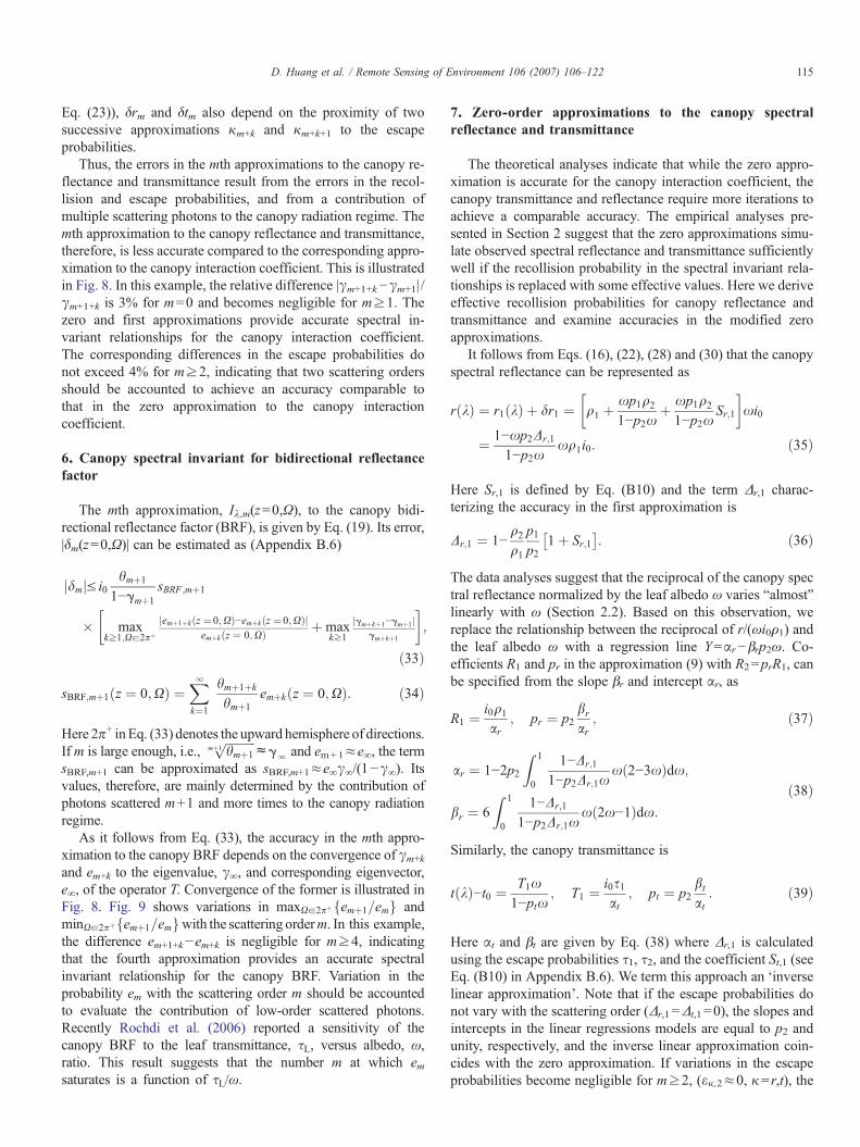
7. Zero-order approximations to the canopy spectralreflectance and transmittance
The theoretical analyses indicate that while the zero appro-ximation is accurate for the canopy interaction coefficient, thecanopy transmittance and reflectance require more iterations toachieve a comparable accuracy. The empirical analyses pre-sented in Section 2 suggest that the zero approximations simu-late observed spectral reflectance and transmittance sufficientlywell if the recollision probability in the spectral invariant rela-tionships is replaced with some effective values. Here we deriveeffective recollision probabilities for canopy reflectance andtransmittance and examine accuracies in the modified zeroapproximations.
It follows from Eqs. (16), (22), (28) and (30) that the canopyspectral reflectance can be represented as
r kð Þ ¼ r1 kð Þ þ dr1 ¼ q1 þxp1q21−p2x
þ xp1q21−p2x
Sr;1
� �xi0
¼ 1−xp2Dr;1
1−p2xxq1i0: ð35Þ
Here Sr,1 is defined by Eq. (B10) and the term Δr,1 charac-terizing the accuracy in the first approximation is
Dr;1 ¼ 1−q2q1
p1p2
1þ Sr;1� �
: ð36Þ
The data analyses suggest that the reciprocal of the canopy spectral reflectance normalized by the leaf albedo ω varies “almost”linearly with ω (Section 2.2). Based on this observation, wereplace the relationship between the reciprocal of r/(ωi0ρ1) andthe leaf albedo ω with a regression line Y=αr−βrp2ω. Co-efficients R1 and pr in the approximation (9) with R2=prR1, canbe specified from the slope βr and intercept αr, as
R1 ¼ i0q1ar
; pr ¼ p2brar
; ð37Þ
ar ¼ 1−2p2Z 1
0
1−Dr;1
1−p2Dr;1xx 2−3xð Þdx;
br ¼ 6Z 1
0
1−Dr;1
1−p2Dr;1xx 2x−1ð Þdx:
ð38Þ
Similarly, the canopy transmittance is
t kð Þ−t0 ¼ T1x1−ptx
; T1 ¼ i0s1at
; pt ¼ p2btat: ð39Þ
Here αt and βt are given by Eq. (38) where Δr,1 is calculatedusing the escape probabilities τ1, τ2, and the coefficient St,1 (seeEq. (B10) in Appendix B.6). We term this approach an ‘inverselinear approximation’. Note that if the escape probabilities donot vary with the scattering order (Δr,1=Δt,1=0), the slopes andintercepts in the linear regressions models are equal to p2 andunity, respectively, and the inverse linear approximation coin-cides with the zero approximation. If variations in the escapeprobabilities become negligible for m≥2, (εκ,2≈0, κ= r,t), the
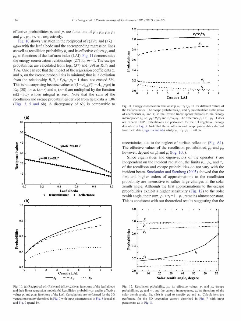
Fig. 11. Energy conservation relationship ρ +τ +p =1 for different values of
116 D. Huang et al. / Remote Sensing of Environment 106 (2007) 106–122
effective probabilities pr and pt are functions of p1, p2, ρ2, ρ1and p1, p2, τ2, τ1, respectively.
Fig. 10 shows variation in the reciprocal of r(λ)/ω and (t(λ)−t0)/ω with the leaf albedo and the corresponding regression linesas well as recollision probability p2 and its effective values, pr andpt, as functions of the leaf area index (LAI). Fig. 11 demonstratesthe energy conservation relationships (27) for m=1. The escapeprobabilities are calculated from Eqs. (37) and (39) as R1/i0 andT1/i0. One can see that the impact of the regression coefficients αrand αt on the escape probabilities is minimal; that is, a deviationfrom the relationship R1/i0+T1/i0+p1= 1 does not exceed 5%.This is not surprising because values of (1−Δκ,1)/(1−Δκ,1p2ω) inEq. (38) for αr (κ=r) and αt (κ= t) are multiplied by the functionω(2−3ω) whose integral is zero. Note that the sum of therecollision and escape probabilities derived from field data is 1.06(Figs. 3, 5 and 6b). A discrepancy of 6% is comparable to
1 1 1
the leaf area index. The escape probabilities ρ1 and τ1 are calculated as the ratiosof coefficients R1 and T1 in the inverse linear approximations to the canopyinterceptance i0, i.e., ρ1=R1/i0 and τ1=R1/i0. The difference ρ1+τ1+p1−1 doesnot exceed +0.05. Calculations are performed for the 3D vegetation canopydescribed in Fig. 7. Note that the recollision and escape probabilities derivedfrom field data (Figs. 3a and 6b) satisfy ρ1+τ1+p1−1=0.06.
Fig. 10. (a) Reciprocal of r(λ)/ω and (t(λ)− i0)/ω as functions of the leaf albedoand their linear regression models. (b) Recollision probability p2 and its effectivevalues pr and pt as functions of the LAI. Calculations are performed for the 3Dvegetation canopy described in Fig. 7 with input parameters as in Fig. 8 (panel a)and Fig. 7 (panel b).
uncertainties due to the neglect of surface reflection (Fig. A1).The effective values of the recollision probabilities, pr and pt,however, depend on βr and βt (Fig. 10b).
Since eigenvalues and eigenvectors of the operator T areindependent on the incident radiation, the limits p∞, ρ∞ and τ∞of the recollison and escape probabilities do not vary with theincident beam. Smolander and Stenberg (2005) showed that thefirst and higher orders of approximations to the recollisionprobability are insensitive to rather large changes in the solarzenith angle. Although the first approximations to the escapeprobabilities exhibit a higher sensitivity (Fig. 12) to the solarzenith angle, their sum, ρ1+τ1=1−p1, remains almost constant.This is consistent with our theoretical results suggesting that the
Fig. 12. Recolision probability, p1, its effective values, pr and pt, escapeprobabilities, ρ1 and τ1, and the canopy interceptance, i0, as functions of thesolar zenith angle. Eq. (26) is used to specify ρ1 and τ1. Calculations areperformed for the 3D vegetation canopy described in Fig. 7 with inputparameters as in Fig. 8.
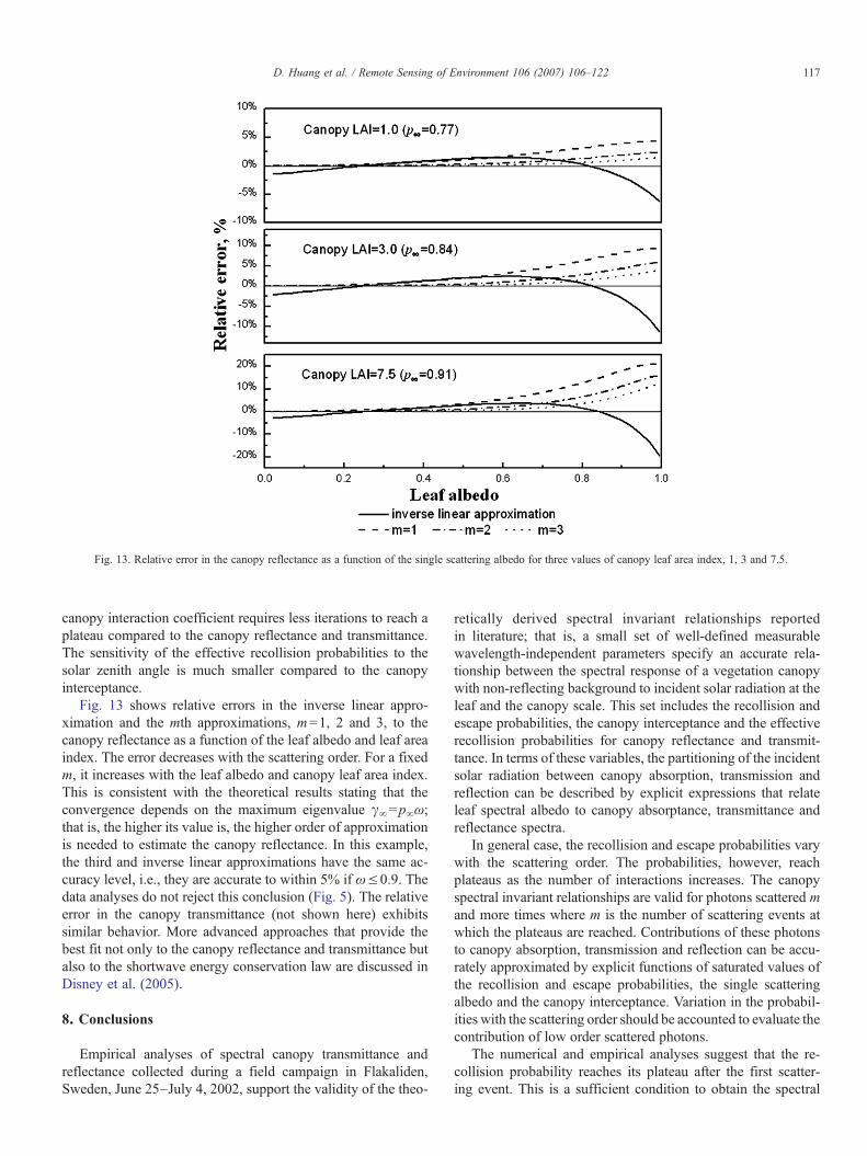
Fig. 13. Relative error in the canopy reflectance as a function of the single scattering albedo for three values of canopy leaf area index, 1, 3 and 7.5.
117D. Huang et al. / Remote Sensing of Environment 106 (2007) 106–122
canopy interaction coefficient requires less iterations to reach aplateau compared to the canopy reflectance and transmittance.The sensitivity of the effective recollision probabilities to thesolar zenith angle is much smaller compared to the canopyinterceptance.
Fig. 13 shows relative errors in the inverse linear appro-ximation and the mth approximations, m=1, 2 and 3, to thecanopy reflectance as a function of the leaf albedo and leaf areaindex. The error decreases with the scattering order. For a fixedm, it increases with the leaf albedo and canopy leaf area index.This is consistent with the theoretical results stating that theconvergence depends on the maximum eigenvalue γ∞=p∞ω;that is, the higher its value is, the higher order of approximationis needed to estimate the canopy reflectance. In this example,the third and inverse linear approximations have the same ac-curacy level, i.e., they are accurate to within 5% if ω≤0.9. Thedata analyses do not reject this conclusion (Fig. 5). The relativeerror in the canopy transmittance (not shown here) exhibitssimilar behavior. More advanced approaches that provide thebest fit not only to the canopy reflectance and transmittance butalso to the shortwave energy conservation law are discussed inDisney et al. (2005).
8. Conclusions
Empirical analyses of spectral canopy transmittance andreflectance collected during a field campaign in Flakaliden,Sweden, June 25–July 4, 2002, support the validity of the theo-
retically derived spectral invariant relationships reportedin literature; that is, a small set of well-defined measurablewavelength-independent parameters specify an accurate rela-tionship between the spectral response of a vegetation canopywith non-reflecting background to incident solar radiation at theleaf and the canopy scale. This set includes the recollision andescape probabilities, the canopy interceptance and the effectiverecollision probabilities for canopy reflectance and transmit-tance. In terms of these variables, the partitioning of the incidentsolar radiation between canopy absorption, transmission andreflection can be described by explicit expressions that relateleaf spectral albedo to canopy absorptance, transmittance andreflectance spectra.
In general case, the recollision and escape probabilities varywith the scattering order. The probabilities, however, reachplateaus as the number of interactions increases. The canopyspectral invariant relationships are valid for photons scattered mand more times where m is the number of scattering events atwhich the plateaus are reached. Contributions of these photonsto canopy absorption, transmission and reflection can be accu-rately approximated by explicit functions of saturated values ofthe recollision and escape probabilities, the single scatteringalbedo and the canopy interceptance. Variation in the probabil-ities with the scattering order should be accounted to evaluate thecontribution of low order scattered photons.
The numerical and empirical analyses suggest that the re-collision probability reaches its plateau after the first scatter-ing event. This is a sufficient condition to obtain the spectral
118 D. Huang et al. / Remote Sensing of Environment 106 (2007) 106–122
invariant for the canopy interaction coefficient that accounts forall scattered photons. The theoretical and numerical analysisindicates the escape probabilities require at least one morescattering event to reach the plateau. The theoretical, numericaland data analyses, however, suggest that the spectral invariantfor canopy reflectance and transmittance can be applied to allscattered photons if one replaces the recollision probability inthe spectral invariant relationships for canopy reflectance andtransmittance with the some effective values. Their accuraciesdepend on the product of the recollision probability and singlescattering albedo; that is, the higher these values are, the lowertheir accuracies. The numerical analysis suggests that therelative errors in the spectral invariant relationships for canopytransmittance and reflectance do not exceed 5% as long as thesingle scattering albedo is below 0.9. The recollision probabil-ity, its effective values and escape probabilities are appeared tobe minimally sensitive to rather large changes in the solar zenithangle.
The probability density that a photon scattered m times willescape the vegetation canopy in a given upward direction con-verges to the wavelength-independent positive eigenvector ofthe transport equation as the number m of interactions increases.This property allows us to formulate the spectral invariant forthe canopy bidirectional reflectance factor; that is, the angularsignature of photons scattered m and more times is proportionalto the positive eigenvector. The coefficient of proportionality isan explicit function of the single scattering albedo, the re-collision probability and the number m of scattering events. Thenumerical analysis suggests that the convergence can beachieved after three to four interactions.
Recall that the spectral invariant relationships are valid forvegetation canopy bounded from below by a non-reflectingsurface. The three-dimensional radiative transfer problem witharbitrary boundary conditions can be expressed as a superpo-sition of the solutions of some basic radiative transfer sub-problems with purely absorbing boundaries to which the spec-tral invariant is applicable (Davis & Knyazikhin, 2005;Knyazikhin & Marshak, 2000; Knyazikhin et al., 2005; Wanget al., 2003). This property and the results of this paper suggestthat spectral response of the vegetation canopy to the incidentsolar radiation can be fully described by a small set of inde-pendent variables which includes spectra of surface reflectanceand leaf albedo, the wavelength-independent canopy intercep-tance, recollision probability, its effective values and escapeprobabilities. This has significant implications for the effectiveexploitation of canopy radiation measurements and modellingmethods. In particular, it allows for the decoupling of the struc-tural and radiometric components of the scattered signal. This inturn permits better quantification and understanding of the struc-tural and biochemical (wavelength-dependent) componentsof the signal, which by necessity are generally considered in acoupled sense.
Acknowledgment
This research was funded by the NASA EOS MODIS andMISR projects under Contracts NNG04HZ09C and 1259071, by
the NASA Earth Science Enterprise under Grant G35C14G2 toGeorgia Institute of Technology. M. Rautiainen and P. Stenbergwere supported by Helsinki University Research Funds.M. Disney and P. Lewis received partial support through theNERC Centre for Terrestrial Carbon Dynamics. We also thankthe anonymous reviewer for her/his comments, which led to asubstantial improvement of the paper.
Appendix A. Field data
A.1. Description of field campaign and measurements
The Flakaliden field campaign was conducted between June25 and July 4, 2002 with the objective of collecting data neededfor validation of satellite derived leaf area index (LAI) andfraction of photosynthetically active radiation (FPAR) absorbedby the vegetation canopy. There were 39 participants from sev-en countries: Sweden, Finland, United States, Italy, Germany,Estonia, and Iceland. Flakaliden is located in northern Sweden,a region dominated by boreal forests. Canopy spectral trans-mittance and reflectance, soil and understorey reflectance spec-tra, needle optical properties, shoot structure and LAI werecollected in six 50 m×50 m plots composed of Norway spruce(Picea abies (L.) Karst) located at Flakaliden Research Area(64°14′N, 19°46′E) operated by the Swedish University ofAgricultural Sciences. Each plot has its own variables andcontrols to determine factors that influence tree growth, i.e.,experimental treatments of the plots involve tree response tovariations in irrigation and fertilization. Data collected in anirrigated and fertilized plot (plot 9A) are used in Section 2.
Simultaneous measurements of spectral up- and downwardradiation fluxes below, and upward radiation fluxes above the50 m×50 m plots from 400 nm to 1000 nm at 1.6 nm spectralresolution were obtained with two ASD hand-held spectro-radiometers (Analytical Spectral Devices Inc., 1999). Ahelicopter was used to take ASD measurements above thecenter of each plot at heights of 15, 30 (used in this study), and45 m. The ASD field of view was set to 25°. A LICOR LI-1800spectroradiometer (LI-COR, 1989) with standard cosinereceptor was placed in an open area to record spectral variationof incident radiation flux density between 300–1100 nm at 1 nmspectral resolution. All spectroradiometers were inter-calibratedby taking a series of simultaneous measurements of downwardfluxes in an open area. We followed the methodology of Wanget al. (2003) to convert the measured spectra to canopy spectralreflectance and transmittance. Note that the spectral measure-ments were made under ambient atmospheric conditions ofdirect and diffuse illumination. This can cause some “spikes” inspectral downward radiation fluxes at the Earth's surface(Fig. 1a), e.g., due to variation in the fraction of the direct ra-diation (Verhoef, 2004). The impact of direct and diffuse com-ponents of the incident radiation on canopy spectral invariantrelationships is discussed in Wang et al. (2003).
Current year, 1-year and 2-year-old spruce needles weresampled from six different heights in the control and irrigatedwith complete fertilizer plots and their transmittances and re-flectance spectra were measured under laboratory conditions
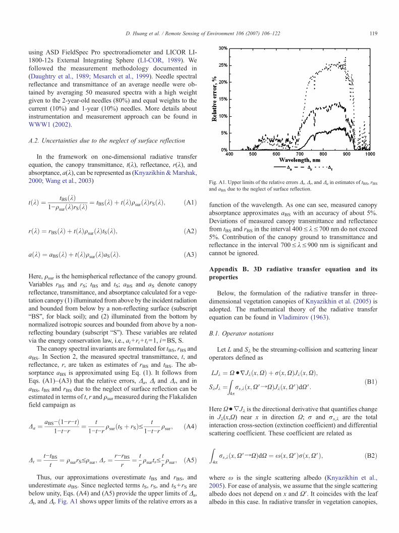
Fig. A1. Upper limits of the relative errors Δt, Δr, and Δa in estimates of tBS, rBSand aBS due to the neglect of surface reflection.
119D. Huang et al. / Remote Sensing of Environment 106 (2007) 106–122
using ASD FieldSpec Pro spectroradiometer and LICOR LI-1800-12s External Integrating Sphere (LI-COR, 1989). Wefollowed the measurement methodology documented in(Daughtry et al., 1989; Mesarch et al., 1999). Needle spectralreflectance and transmittance of an average needle were ob-tained by averaging 50 measured spectra with a high weightgiven to the 2-year-old needles (80%) and equal weights to thecurrent (10%) and 1-year (10%) needles. More details aboutinstrumentation and measurement approach can be found inWWW1 (2002).
A.2. Uncertainties due to the neglect of surface reflection
In the framework on one-dimensional radiative transferequation, the canopy transmittance, t(λ), reflectance, r(λ), andabsorptance, a(λ), can be represented as (Knyazikhin &Marshak,2000; Wang et al., 2003)
t kð Þ ¼ tBSðkÞ1−qsurðkÞrSðkÞ
¼ tBS kð Þ þ t kð Þqsur kð ÞrS kð Þ; ðA1Þ
rðkÞ ¼ rBSðkÞ þ tðkÞqsurðkÞtSðkÞ; ðA2Þ
aðkÞ ¼ aBSðkÞ þ tðkÞqsurðkÞaSðkÞ: ðA3Þ
Here, ρsur is the hemispherical reflectance of the canopy ground.Variables rBS and rS; tBS and tS; aBS and aS denote canopyreflectance, transmittance, and absorptance calculated for a vege-tation canopy (1) illuminated from above by the incident radiationand bounded from below by a non-reflecting surface (subscript“BS”, for black soil); and (2) illuminated from the bottom bynormalized isotropic sources and bounded from above by a non-reflecting boundary (subscript “S”). These variables are relatedvia the energy conservation law, i.e., ai+ri+ ti=1, i=BS, S.
The canopy spectral invariants are formulated for tBS, rBS andaBS. In Section 2, the measured spectral transmittance, t, andreflectance, r, are taken as estimates of rBS and tBS. The ab-sorptance aBS is approximated using Eq. (1). It follows fromEqs. (A1)–(A3) that the relative errors, Δa, Δt and Δr, and inaBS, tBS and rBS due to the neglect of surface reflection can beestimated in terms of t, r and ρsur measured during the Flakalidenfield campaign as
Da ¼ aBS−ð1−r−tÞ1−t−r
¼ t
1−t−rqsur tS þ rSð ÞV t
1−t−rqsur; ðA4Þ
Dt ¼ t−tBSt
¼ qsurrSVqsur; Dr ¼ r−rBSr
¼ trqsurtsV
trqsur; ðA5Þ
Thus, our approximations overestimate tBS and rBS, andunderestimate aBS. Since neglected terms tS, rS, and tS+ rS arebelow unity, Eqs. (A4) and (A5) provide the upper limits of Δa,Δt, and Δr. Fig. A1 shows upper limits of the relative errors as a
function of the wavelength. As one can see, measured canopyabsorptance approximates aBS with an accuracy of about 5%.Deviations of measured canopy transmittance and reflectancefrom tBS and rBS in the interval 400≤λ≤700 nm do not exceed5%. Contribution of the canopy ground to transmittance andreflectance in the interval 700≤λ≤900 nm is significant andcannot be ignored.
Appendix B. 3D radiative transfer equation and itsproperties
Below, the formulation of the radiative transfer in three-dimensional vegetation canopies of Knyazikhin et al. (2005) isadopted. The mathematical theory of the radiative transferequation can be found in Vladimirov (1963).
B.1. Operator notations
Let L and Sλ be the streaming-collision and scattering linearoperators defined as
LJk ¼ X •jJkðx;XÞ þ rðx;XÞJkðx;XÞ;SkJk ¼
Z4prs;kðx;XVYXÞJkðx;XVÞdXV:
ðB1Þ
Here Ω•∇Jλ is the directional derivative that quantifies changein Jλ(x,Ω) near x in direction Ω; σ and σs,λ are the totalinteraction cross-section (extinction coefficient) and differentialscattering coefficient. These coefficient are related as
Z4prs;kðx;XVYXÞdX ¼ xðx;XVÞrðx;XVÞ; ðB2Þ
where ω is the single scattering albedo (Knyazikhin et al.,2005). For ease of analysis, we assume that the single scatteringalbedo does not depend on x and Ω′. It coincides with the leafalbedo in this case. In radiative transfer in vegetation canopies,
120 D. Huang et al. / Remote Sensing of Environment 106 (2007) 106–122
the extinction coefficient does not depend on the wavelength(Ross, 1981).
B.2. Boundary conditions
Let the domain V be illuminated by a parallel beam of unitintensity. Interaction of shortwave radiation with the vegetationcanopy in V is described by the following boundary value prob-lem for the 3D radiative transfer equation (Knyazikhin et al.,2005; Ross, 1981)
LJk ¼ SkJk; ðB3Þ
Jkðxb;XÞ ¼ dðX−X0Þ; xbadV ; X •nbb0: ðB4Þ
Here Ω0 is the direction of the incident beam; nb is the outwardnormal at point xb∈δV, and Jλ(x,Ω) is the monochromaticintensity which depends on the wavelength, λ, location x anddirection Ω. The flux, F↓, of radiation incident on the canopyboundary is given by FA ¼ RdV jnb •X0jHð−nb •X0Þdrb whereH is the Heaviside function. For boundary conditions used inSection 5, F↓= |μ0|δVt where μ0 is the cosine of the polar angleof Ω0 and δVt is the area of the canopy upper boundary. Theboundary condition for the lower boundary is set to zero. Underconditions (i)–(iii) (see Section 3), the intensity, Iλ(x,Ω), ofradiation field in V is given by the solution of the boundaryvalue problem (B3) and (B4) normalized by F↓, i.e., Iλ=Jλ/F
↓.
B.3. Comments on Eq. (17)
In the framework of functional analysis, Eq. (13) is a norm inthe Banach space of integrable functions, and T is a linearoperator acting in this space. Eq. (17) are valid for any linearoperator satisfying some general conditions (Riesz & Sz.-Nagy,1990) which are met for the three-dimensional transport equa-tion (Vladimirov, 1963) and Monte Carlo models of the ra-diative transfer (Marchuk et al., 1980).
B.4. Eigenvectors and eigenvalues of the radiative transferequation
An eigenvalue of the radiative transfer equation is a number γsuch that there exists a function e(x,Ω) that satisfies γLe=Sλe andzero boundary conditions. Since the eigenvalue and eigenvectorproblem is formulated for zero boundary conditions, γ and e(x,Ω)are independent on the incoming radiation. Under some generalconditions (Vladimirov, 1963), the set of eigenvalues andeigenvectors is a discrete set. The radiative transfer equation hasa unique positive eigenvalue, γ∞, that corresponds to a uniquepositive eigenvector, e∞ (Vladimirov, 1963).
B.5. Successive orders of scattering approximations
The intensity, Iλ(x,Ω), satisfies the integral radiative transferequation Iλ=TIλ+Q0 (Knyazikhin et al., 2005). Here T=L
−1Sλ,and Q0 satisfies LQ0=0 and the boundary conditions (B4)normalized by the incident flux F↓. The boundary conditions
and the streaming-collision operator do not depend on wave-length, and thus, Q0 is wavelength independent. The solutionIλ=(E−T )−1Q0 to the integral radiative transfer equation canbe expanded in the Neumann series (12) where Qm=T
mQ0
satisfies the equation LQm=SλQm−1 and zero boundary con-ditions. The symbol E denotes the identity operator. Integratingthis equation over spatial and directional variables and takinginto account Eq. (B2), one obtains the following energy con-servation relationships
jjTmQ0jjr þ jjTmQ0jjt þ jjTmQ0jj ¼ xjjTm−1Q0jj: ðB5Þ
Eq. (27) is obtained by dividing Eq. (B5) by ω||Tm−1Q0||.It follows from Eqs. (26) and (14) that
qm ¼ 1x
jjTmQ0jjrjjTm−1Q0jj ¼
1x
jjTmQ0jjjjTm−1Q0jj
jjTmQ0jjrjjTmQ0jj
¼ gmx
jjemjjr: ðB6Þ
This equation can be rewritten as ||em||r=ωρm/γm. Similarly,||em||t=ωτm/γm.
B.6. Error in the mth approximation
It follows from Eq. (14) that
gmþ1emþ1 ¼ jjQmþ1jjjjQmjj
Qmþ1
jjQmþ1jj ¼TQm
jjQmjj ¼ Tem: ðB7Þ
Taking into account the operator identityPlk¼0
Tk ¼ ðE−TÞ−1and Eq. (B7), one gets
dm ¼ Ik x;Xð Þ−Ik;m x;Xð Þ
¼ TXlk¼0
Tk
!TmQ0−jjQmjj gmþ1
1−gmþ1emþ1
¼ jjQmjj½TðE−TÞ−1
em−1
1−gmþ1Tem�
¼ jjQmjjTðE−TÞ−1½em− 11−gmþ1
E−Tð Þem�¼ jjQmjjTðE−TÞ−1½em− 1
1−gmþ1em þ gmþ1emþ1
1−gmþ1�
¼ jjQmjj gmþ1
1−gmþ1
Xlk¼1
Tkemþ1−Tkem� �
:
It follows from Eqs. (B7) and (22) that
dm ¼ i0hmþ1
1−gmþ1
Xlk¼1
hmþkþ1
hmþ1emþkþ1−
gmþ1
gmþ1þkemþk
¼ i0hmþ1
1−gmþ1
Xlk¼1
hmþkþ1
hmþ1emþkþ1−emþk þ gmþ1þk−gmþ1
gmþ1þkemþk
:
ðB8Þ
The upper bound to the error δm follows directly from Eq. (B8).
121D. Huang et al. / Remote Sensing of Environment 106 (2007) 106–122
Let κ and κm represent either canopy reflectance (κ= r, κm=ρm) or canopy transmittance (κ= t, κm=τm). Integrating δm|μ|over the upward (downward) directions and taking into accountEqs. (22), (26) and (B6) one gets
djm ¼ jjdmjjj¼ i0
hmþ1
1−gmþ1
Xlk¼1
hmþkþ1
hmþ1jjemþkþ1jjj−
gmþ1
gmþ1þkjjemþk jjj
¼ i0hm
1−gmþ1
Xlk¼1
hmþkþ1
hm
xjmþ1þk
gmþ1þk−
gmþ1
gmþ1þk
xjmþk
gmþk
¼ xi0hm
1−gmþ1
Xlk¼1
hmþk
hmjmþ1þk−
gmþ1
gmþkjmþk
¼ xi0hmjmþ1
1−gmþ1
Xlk¼1
hmþk
hm
jmþk
jmþ1
jmþ1þk
jmþk−gmþ1
gmþk
¼ xi0hmjmþ1
1−gmþ1Sj;m;
ðB9Þwhere
Sj;m ¼Xlk¼1
hmþk
hm
jmþk
jmþ1
jmþ1þk−jmþk
jmþkþ gmþk−gmþ1
gmþk
:
ðB10ÞIt follows from Eq. (B10) that |Sκ,m|≤ (εκ,m+1+εγ,m+1)sκ,m.
Estimate (23) can be obtained in a similar manner.
Appendix C. Simulation of the 3D canopy radiation regime
The domain V is a parallelepiped of horizontal dimensionsXd, Yd, and height H. The top, δVt, bottom, δVb, and lateral,δVl, surfaces of the parallelepiped form the canopy boundaryδV. Trees in V are represented by cylinders with the base radiusrB and the height H. Non-dimensional scattering centres(leaves) are assumed to be uniformly distributed and spatiallyuncorrelated within tree crowns. The extinction coefficienttakes on values σ(Ω) and zero within and outside the treecrowns, respectively. The centres of crown bases are scatteredon δVb according to a stationary Poisson point process ofintensity d. The amount of leaf area in the tree crown isparameterized in terms of the plant LAI, L0, defined as thetotal half leaf (needle) area in the tree crown normalized by thecrown base area πrB
2. In the Flakaliden research area, its valuevaries between 5 and 15. The canopy LAI is gL0 where g=1−exp(−πrB2d ) is the ground covered by vegetation (Huang etal., in press). A uniform and bi-Lambertian models areassumed for the leaf normal distribution and the diffuse leafscattering phase function, respectively (Knyazikhin et al.,2005; Ross, 1981). Leaf hemispherical reflectance andtransmittance are assumed to have the same value. Thestochastic radiative transfer equation is used to obtain verticalprofiles of horizontally averaged 3D radiation field Iλ(x,Ω)(Huang et al., in press; Shabanov et al., 2000). A detaileddescription of the stochastic model used in our simulations canbe found in Huang et al. (in press).
References
Analytical Spectral Devices (ASD), Inc. (1999). ASD technical guide (4th ed.).Boulder, CO, USA: ASD Inc.
Bonan, G. B., Oleson, K. W., Vertenstein, M., Levis, S., Zeng, X., Dai, Y., et al.(2002). The land surface climatology of the community land model coupledto the NCAR community climate model. Journal of Climate, 15,3123−3149.
Buermann, W., Dong, J., Zeng, X., Myneni, R. B., & Dickinson, R. E. (2001).Evaluation of the utility of satellite based vegetation leaf area index data forclimate simulations. Journal of Climate, 14(17), 3536−3550.
Daughtry, C. S. T., Biehl, L. L., & Ranson, K. J. (1989). A new technique tomeasure the spectral properties of conifer needles. Remote Sensing ofEnvironment, 27, 81−91.
Davis, A. B., & Knyazikhin, Y. (2005). A primer in three-dimensional radiativetransfer. In A. Marshak & A.B. Davis (Eds.), Three-dimensional radiativetransfer in the cloudy atmosphere (pp. 153−242). Springer-Verlag.
Dickinson, R. E, Henderson-Sellers, A., Kennedy, P. J., & Wilson, M. F. (1986).Biosphere atmosphere transfer scheme (BATS) for the NCAR communityclimate model. NCAR technical note, NCAR, TN275+STR 69 pp.
Disney, M., Lewis, P., Quaife, T., & Nichol, C. (2005). A spectral invariantapproach to modeling canopy and leaf scattering. Proc. the 9th InternationalSymposium on Physical Measurements and Signatures in Remote Sensing(ISPMSRS), 17–19 October 2005, Beijing, China, Part 1(pp. 318-320).
Disney, M., Lewis, P., & Saich, P. (2006). 3D modeling of forest canopystructure for remote sensing simulations in the optical and microwavedomains. Remote Sensing of Environment, 100, 114−132.
Huang, D., Knyazikhin, Y., Wang, W., Deering, D. W., Stenberg, P., Shabanov,N., et al. (in press). Stochastic transport theory for investigating the three-dimensional canopy structure from space measurements. Remote Sensing ofEnvironment.
Kiehl, J. T., Hack, J. J., Bonan, G. B., Boville, B. A., Briegleb, B. P.,Williamson, D. L., et al. (1996). Description of the NCAR communityclimate model (CCM3). Tech. Rep. NCAR/TN-420+STR., National Centerfor Atmospheric Research, Boulder, CO, 152 pp. [Available fromNCAR, P.O.Box 3000, Boulder, CO 80307.]
Kiehl, J. T., Hack, J. J., Bonan, G. B., Boville, B. A., Williamson, D. L., &Rasch, P. J. (1998). The National Center for Atmospheric Research com-munity climate model: CCM3. Journal of Climate, 11, 1131−1149.
Knyazikhin, Y., & Marshak, A. (2000). Mathematical aspects of BRDFmodelling: Adjoint problem and Green's function. Remote Sensing Reviews,18, 263−280.
Knyazikhin, Y., Marshak, A., & Myneni, R. B. (2005). Three-dimensionalradiative transfer in vegetation canopies and cloud–vegetation interaction. InA. Marshak & A.B. Davis (Eds.), Three-dimensional radiative transfer inthe cloudy atmosphere (pp. 617−652). Springer-Verlag.
Knyazikhin, Y., Martonchik, J. V., Myneni, R. B., Diner, D. J., & Running, S. W.(1998). Synergistic algorithm for estimating vegetation canopy leaf area indexand fraction of absorbed photosynthetically active radiation from MODIS andMISR data. Journal of Geophysical Research, 103, 32257−32274.
Lewis, P., & Disney, M. (1998). The botanical plant modeling system (BPMS): acase study of multiple scattering in a barley canopy. Proc. IGARSS'98,Seattle, USA.
Lewis, P., Hillier, J., Watt, J., Andrieu, B., Fournier, C., Saich, P., et al. (2005).3D dynamic vegetation modeling of wheat for remote sensing and inversion.Proc. the 9th International Symposium on Physical Measurements andSignatures in Remote Sensing (ISPMSRS), 17–19 October 2005, Beijing,China, Part 1(pp. 144-146).
Lewis, P., Saich, P., Disney, M., Andrieu, B., & Fournier, C. (2003). Modeling theradiometric response of a dynamic, 3D structural model of wheat in the opticaland microwave domains. Proc. IEEE Geoscience and Remote SensingSymposium. IGARSS'03, 21–25 July 2003, Toulouse, Vol. 6 (3543−3545).
Li-COR. (1989). LI-1800 portable spectroradiometer instruction manual.Lincoln, NE, USA: Li-COR.
Marchuk, G. I., Mikhailov, G. A., Nazaraliev, M. A., Darbinjan, R. A., Kargin,B. A., & Elepov, B. S. (1980). The Monte Carlo methods in atmosphericoptics. New York: Springer-Verlag. 208 pp.
122 D. Huang et al. / Remote Sensing of Environment 106 (2007) 106–122
Mesarch,M.A., Walter-Shea, E.A., Asner, G. P., Middleton, E.M., & Chan, S. S.(1999). A revised measurement methodology for conifer needles spectraloptical properties: evaluating the influence of gaps between elements. RemoteSensing of Environment, 68, 177−192.
Myneni, R. B., Hoffman, S., Knyazikhin, Y., Privette, J. L., Glassy, J., Tian,Y., et al. (2002). Global products of vegetation leaf area and fractionabsorbed par from year one of MODIS data. Remote Sensing ofEnvironment, 83, 214−231.
Panferov, O., Knyazikhin, Y., Myneni, R. B., Szarzynski, J., Engwald, S.,Schnitzler, K. G., et al. (2001). The role of canopy structure in the spectralvariation of transmission and absorption of solar radiation in vegetationcanopies. IEEE Transactions onGeoscience and Remote Sensing, 39, 241−253.
Potter, C. S., Randerson, J. T., Field, C. B., Matson, P. A., Vitousek, P. M.,Mooney, H. A., et al. (1993). Terrestrial ecosystem production: A processmodel based on global satellite and surface data. Global BiogeochemicalCycles, 7(4), 811−841.
Raich, J. W, Rastetter, E. B, Melillo, J. M, Kicklighter, D. W, Steudler, P. A,Peterson, B. J, et al. (1991). Potential net primary productivity in SouthAmerica: Application of a global model.Ecological Applications, 1, 399−429.
Rautiainen, M., & Stenberg, P. (2005). Application of photon recollisionprobability in coniferous canopy reflectance model. Remote Sensing ofEnvironment, 96, 98−107.
Riesz, F., & Sz.-Nagy, B. (1990). Functional analysis. New York: DoverPublication, Inc. 504 pp.
Rochdi, N., Fernandes, R., & Chelle, M. (2006). An assessment of needlesclumping within shoots when modeling radiative transfer within homoge-neous canopies. Remote Sensing of Environment, 102, 116−134.
Ross, J. (1981). The radiation regime and architecture of plant stands Norwell,MA: Dr. W. Junk (pp.391).
Running, S. W., & Hunt Jr., E. R. (1993). Generalization of a forest ecosystemprocessmodel for other biomes, BIOME-BGC, and an application for global-scale models. In J. R. Ehleringer & C. B. Field (Eds.), Scaling physiologicalprocesses: Leaf to globe (pp. 141−157). San Diego: Academic Press.
Saich, P., Lewis, P., Disney, M. I., van Oevelen, P., Woodhouse, I., Andrieu, B.,et al. (2003). Development of vegetation growth models for remote sensingapplications. Final report of ESA contract AO/1-3679/00/NL/NB (availablefrom www.geog.ucl.ac.uk/~psaich/esa/fullindex.htm)
Sellers, P. J., Mintz, Y., Sud, Y. C., & Dalcher, A. (1986). A simple biospheremodel (SiB) for use within general circulation. Journal of AtmosphereScience, 43.
Shabanov, N. V., Knyazikhin, Y., Baret, F., & Myneni, R. B. (2000). Stochasticmodeling of radiation regime in discontinuous vegetation canopies. RemoteSensing of Environment, 74(1), 125−144.
Shabanov, N. V., Wang, Y., Buermann, W., Dong, J., Hoffman, S., Smith, G.,et al. (2003). The effect of spatial heterogeneity in validation of the MODISLAI and FPAR algorithm over broadleaf forests. Remote Sensing ofEnvironment, 85, 410−423.
Smolander, S., & Stenberg, P. (2005). Simple parameterizations of the radiationbudget of uniform broadleaved and coniferous canopies. Remote Sensing ofEnvironment, 94, 355−363.
Tian, Y., Wang, Y., Zhang, Y., Knyazikhin, Y., Bogaert, J., & Myneni, R. B.(2003). Radiative transfer based scaling of LAI/FPAR retrievals fromreflectance data of different resolutions. Remote Sensing of Environment, 84(1), 143−159.
Verhoef, W. (2004). Extension of SAIL to model solar-induced canopyfluorescence spectra. 2nd International Workshop on Remote Sensing ofVegetation Fluorescence, Nov. 2004, Montreal, Canada.
Vladimirov, V. S. (1963). Mathematical problems in the one-velocity theory ofparticle transport. Tech. Rep. AECL-1661, At. Energy of Can. Ltd., ChalkRiver, Ontario, 302 pp.
Wang, Y., Buermann,W., Stenberg, P., Smolander, H., Häme, T., Tian, Y., et al.(2003). A new parameterization of canopy spectral response to incident solarradiation: Case study with hyperspectral data from pine dominant forest.Remote Sensing of Environment, 85, 304−315.
WWW1: Report on Flakaliden field campaign, Sweden, June 25–July 4, 2002.http://cybele.bu.edu/modismisr/validation/expts.html