Canary in a Coal Mine: Impact of Mid-20th CenturyAir Pollution on Infant Mortality and Property Values ∗

Karen Clay, Carnegie Mellon University and NBERJoshua Lewis, University of Montreal

Edson Severnini, Carnegie Mellon University and IZA

November 28, 2015

Abstract

This paper uses the mid-20th century expansion in U.S. coal-fired electricity generation tostudy the local impact of air pollution on infant mortality and housing prices. The empiricalanalysis exploits the timing of coal-fired power plant openings and annual variation in plant-level coal consumption in the U.S. from 1938 to 1962. The estimates suggest that the rise inpower plant coal consumption was responsible for an additional 3,500 infant deaths per yearby the end of the sample period. We examine whether individuals perceived these healthcosts. Although hedonic estimates of the average marginal willingness to pay for clean airare close to zero, there is substantial heterogeneity in the housing market response. At lowlevels of electricity access, expansions in coal-fired electricity generation have positive effectson housing prices. At high levels of electricity access, this relationship is negative. Theseresults suggest that households traded off the pollution costs of coal-fired power against thebenefits of low-cost electricity.

∗We thank Martha Bailey, Leah Boustan, Antonio Bento, Claudia Goldin, Michael Haines, Walker Han-lon, Matthew Kahn, Nicolai Kuminoff, Alberto Salvo, Joseph Shapiro, and seminar participants at the 61thAnnual North American Meetings of the Regional Science Association International, the 2015 Annual Meet-ing of the Population Association of America, the 2015 NBER DAE Spring Meetings, and UCLA for valuablecomments and suggestions.Karen Clay: Mailing address: Carnegie Mellon University, 5000 Forbes Ave., Pittsburgh, PA 15213, Phone:(412) 268-4197, Email: kclay@andrew.cmu.eduJoshua Lewis: Mailing address: Universite de Montreal, 3150, rue Jean-Brillant, Montreal, QC, H3T 1N8,Phone: (514) 240-4972, Email: joshua.lewis@umontreal.ca.Edson Severnini: Mailing address: Carnegie Mellon University, 4800 Forbes Ave, Pittsburgh, PA 15213,Phone: (510) 860-1808, Email: ersevernini@gmail.com.

1 Introduction

Today, air quality is highly valued in the U.S. and other developed nations (e.g., Chay

and Greenstone, 2005). This is likely due to the preponderance of evidence on the harmful

effects of pollution (e.g., Chay and Greenstone, 2003a, 2003b; Currie and Neidell, 2005).

Historically, however, it is unclear the extent to which the public perceived these health

risks, a situation analogous to developing countries nowadays. The lack of an effective air

quality management system prior to the passage of major legislations such as the 1963 Clean

Air Act made it difficult to (i) establish a link between air pollution and health, and (ii) assess

the value of environmental amenities. As a byproduct of economic growth, air pollution was

associated with tangible benefits hard to disentangle from potentially hidden health costs.

The expansion of the power grid in the U.S. around mid-20th century presents a unique

opportunity to examine these issues, and may provide guidance for policymaking in the

current energy challenge faced by developing countries (Greenstone and Jack, 2015). First,

the opening of a number of coal-fired power plants in the 1940s and 1950s allows for the

credibly estimation of the impact of local air pollution on infant mortality during a period

of unregulated and unmonitored emissions. Second, coal-fired power had clear tradeoffs:

benefits from electricity generation and health costs due to air pollution. Third, the time

frame precedes landmark epidemiological studies on the health effects of air pollution by

several decades (Lave and Seskin, 1970; Pope, 1991), so citizens were unlikely to have full

information of the health risks posed by coal-fired emissions.

This paper uses newly digitized annual administrative data on power plants from 1938 to

1962 to examine the effects of the rapid expansion of electricity generation on infant mortality

and housing values. We first establish the link between coal-fired power generation and

mortality by exploiting (i) the timing of power plant openings, and (ii) the annual variation

on plant-level coal consumption and generating capacity. We then estimate hedonic models

to assess the extent to which the public perceived those health risks and whether households

traded off the costs and benefits of coal powered electricity.

1

The first research design is based on the timing of power plant openings. Guided by

the literature on pollution transport, we identify a ‘treatment’ radius of 30 miles around

a plant.1 The analysis compares the relative outcomes in counties within this radius to

outcomes in counties slightly farther away, before and after a plant opening. Because both

treatment and control counties benefited similarly from the electricity produced by these

plants, these models identify the cost of pollution, net of the gains associated with increased

electricity production. The second empirical strategy exploits spatial and temporal variation

in annual coal consumption generating capacity by electric utilities, in a county fixed effects

framework. These models capture the net impact of both the costs and benefits of local coal-

fired generation for health and property values. Importantly, we estimate these relationships

at different levels of baseline electricity access, which allows us to disentangle these two

opposing forces.

We find that coal-fired electricity generation had substantial negative effects on health.

The opening of a large fossil fuel power plant (>75mw) is associated with a 2 percent

increase in infant mortality. On average, the costs of air pollution overwhelm the health

benefits associated with electricity access, and our estimates imply that the rise in coal-fired

electricity generation between 1938 and 1962 was responsible for an additional 3,500 infant

deaths per year by 1962.

Despite the large health impacts, average housing values did not respond to local power

plant coal consumption. The estimates for households’ willingness-to-pay to avoid pollution

are small and statistically insignificant. Given imperfect information, the estimates may

understate the true costs of this local externality. Alternatively, the null result could reflect

a tradeoff between the health costs and the economic gains of electricity access. To shed

light on this question, we evaluate the impact of power plant coal consumption at different

levels of baseline electricity access. Local coal consumption has positive and statistically

significant effects on housing prices at low levels of access and negative and statistically

1See section 2.1 for a detailed discussion.

2

significant effects at high levels of access. These effects mirror the relationship between

electric utility coal consumption and infant mortality at different levels of electricity access.

Together the findings suggest that households were able to infer the health costs associated

with coal-fired emissions, despite a lack of direct evidence on this relationship. Nevertheless

the housing market response is substantially smaller than would be predicted based on the

standard value of a statistical life (VSL) for this period (Costa and Kahn, 2004), suggesting

that information on these health risks was at best incomplete.

This paper makes three main contributions to the literature. First, it sheds light on

the effects of local air pollution on health in a setting with virtually no environmental

regulation and a poorly informed public. Previous work has focused on the post-Clean Air

Act period, when the public was better informed of these health effects and pollution levels

were significantly lower. Influential studies such as Chay and Greenstone (2003a, 2003b) and

Currie and Neidell (2005) either exploit Clean Air Act regulations to uncover health effects of

pollution, or focus on post-CAAA periods.2 Perhaps the closest studies to ours are Hanlon

(2015a) and Hanlon and Tian (2015) on the mortality associated with coal consumption

in manufacturing in the 19th century England, and Barreca, Clay and Tarr (2014) on the

mortality effects of coal burning for home heating in mid-20th century U.S.

Second, this study offers a new methodology for evaluating local air quality in settings in

which direct pollution monitors are unavailable. This strategy complements other innovative

approaches recently used in the developing context. For example, Jayachandran (2009) uses

satellite aerosol monitoring data to measuring the missing children associated with extreme

pollution exposure during infancy and in utero due to forest fires in Indonesia. Arceo-

Gomez, Hanna, and Oliva (forthcoming) use the frequency of thermal inversions, which trap

pollutants close to the ground, to assess the impact of pollution exposure on infant mortality

in Mexico City. Almond et al. (2009) and Chen et al. (2013) use the geographic discontinuity

2Other studies such as Currie and Walker (2011), Currie et al. (2015), Schlenker and Walker (forth-coming), and Severnini (2015) use air pollution shocks that might not be fully perceived by the public toestimate their impact on health, but are all in settings with some type of emission control.

3

created by a Chinese policy to subsidize coal north of the Huai River to estimate the effect

of particulate matter on life expectancy.

Third, the paper adds to recent work assessing the reliability of the hedonic method (see

Currie et al, 2015). Our results show that standard WTP estimates for air quality can yield

puzzling results when amenities arising directly from pollution-intensive activities are not

accounted for. Conflicting estimates of the willingness to pay for air quality might be due

to omission of amenities generated directly by pollution.3

More broadly, the paper relates to the literature on the effects of electrification, and on

the historical development of the American economy. While a growing body of research has

focused on the benefits of electrification to female employment (Dinkelman, 2011; Lewis,

2014a), local development (Lipscomb, Mobarak, and Bahram, 2013; Severnini, 2014), agri-

cultural output (Fishback and Kitchens, forthcoming), health (Lewis, 2014b), and man-

ufacturing productivity (Allcott, Collard-Wexler and O’Connell, forthcoming), our study

highlights the potential pollution costs associated with increasing electricity access. Simi-

larly, while the role of transportation infrastructure in transforming the American economy

in the 19th and 20th centuries has been studied intensively (Fogel, 1964; Haines and Margo,

2008; Atack et al., 2010; Atack and Margo, 2011; Atack, Haines and Margo, 2011; Donaldson

and Hornbeck, forthcoming; Baum-Snow, 2007; Michaels, 2008), the expansion of the U.S.

power grid has been overlooked.

This paper proceeds as follows: Section 2 discusses the history of electrification in the

United States. Section 3 describes the data. Section 4 presents our empirical framework.

Section 5 reports our findings, and Section 6 concludes.

3In a related study, Hanlon (2015b) shows that omission of coal consumption by manufacturing in theestimation of city growth models could lead to misleading findings. Industrial activity may create jobs andpull workers from other places, but it might also emit tons of pollutants that push workers away.

4

2 Historical Background

2.1 Coal-fired Electricity, Pollution, and Health

Coal-fired electricity generation rose substantially during the mid-20th century. Between

1938 and 1962, 154,255 MW of electricity capacity were added, over 80 percent of which

was coal powered.4 Most of the growth occurred as new bigger plants were built and older,

smaller plants were taken offline. In fact, despite the larger increases in capacity, the total

number of electric utility plants actually fell from 3,903 in 1938 to 3,402 in 1963.5

With these expansions in coal-fired capacity, electric utilities became an increasingly

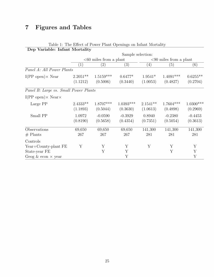
important source of domestic coal consumption. Figures 1 and 2 show that coal consumption

for electricity generation grew rapidly and was a rising share of overall consumption. Coal

consumption was 38.4 million short tons in 1938 and 211.3 million short tons in 1963. Coal

consumption grew rapidly, but less rapidly than kilowatts generated (5.5 times vs. 8.1 times),

because newer larger plants were more efficient than older smaller plants. 97 percent of the

coal used was bituminous coal.6 As a share of overall consumption, coal consumption for

electricity generation rose from 10 percent to 50 percent, as other uses such as coal for home

heating and coal for railways declined.

The combustion of coal produces a number of air pollutants, such as sulfur dioxide,

nitrogen oxides, and particulate matter. A large literature has shown that these pollutants

have negative effects on both infant and all-age mortality.7 For infants, particulates affect

health through both prenatal exposure (Curry and Walker, 2011), and postnatal exposure

(Woodruff et al, 2008; Arceo-Gomez et al, 2012).

Prior to the passage of the 1963 Clean Air Act, electric utilities did little to mitigate

4United States Bureau of the Census (1976), p.824.5United States Bureau of the Census (1975), Series S53-54.6Anthracite coal by use is only reported beginning in 1954. In 1954 it was 3 percent and it remained

small through 1963. United States Bureau of Mines, Minerals Yearbook (1958), Table 38 (anthracite), p.188. Table 53 (bituminous), p. 102.

7See Chay and Greenstone (2003a, 2003b), Currie and Neidell (2005) for the effects on infant mortality;Clay and Troesken (2010), Pope et al (1992), Clancy et al (2002), Hedley et al (2002), and Pope et al (2007),for the effects on all-age mortality.

5

the consequences of the air pollution. Experimentation with scrubbing did not begin until

the late 1960s in the United States (Biondo and Marten, 1977). The height of power plant

smoke stacks – a key determinant of pollutant dispersion – was relatively constant from 1938

to 1962 (see Figure 3). The primary mitigation of pollution came from siting of the plants

further from population centers, as advances in transmission technology allowed electricity

to be shipped over longer distances. Figure 4 displays the density of thermal capacity around

the 50 largest cities in the United States.8 In both time period, the largest mass of plants

are concentrated within 75 miles of the city-centroids. Nevertheless, the distribution flattens

by 1960, as a larger share of power plants was located further away from city centers.

The extent to which this rise in power plant coal consumption affected the health of

the local population depends on local weather conditions, plant characteristics, and the

properties of the pollutant in question. Fortunately, previous research on pollution transport

provides some guidance on the dispersion of these pollutants. Particulate matter, widely

considered the most hazardous pollutant associated with fossil fuel combustion, tends to

be locally concentrated. Figure 5 plots the average density of PM2.5 by distance to the

source, based on study of nine large power plants in Illinois in 1998 (Levy et al., 2002).9

The relationship between distance and PM2.5 exposure is highly nonlinear. Over 40 percent

of PM2.5 exposure occurs within 30 miles of the plant; less than 20 percent occurs at a

distance between 30 and 90 miles. When differences in land area are taken into account,

these differences are even starker: the average person within 30 miles of a plant is exposed

to concentration of PM2.5 that is 11 times higher than the level of exposure of an individual

located between 30 and 60 miles from a plant. As a result, health effects associated with

power plant coal consumption should be concentrated locally.10

8Because area increases with the square of distance, the figure is constructed so that a uniform distribu-tion would appear as a flat line in the figure.

9These grandfathered power plants were not subject to emissions regulation. Average stack height forthese plants was 132 meters, slightly higher than those in our sample.

10On the other hand, secondary pollutants such as sulfur dioxide and nitrogen oxides are diluted in theatmosphere and carried further away. For example, Levy and Spengler (2002) find that exposure to thesepollutants decreases linearly with distance between 0 and 500 kilometers.

6

Coal-fired electricity offered a range of local benefits. Access to electricity is linked to

decreases in infant mortality (Lewis 2015, Gohlke 2011).11 Figure 6 provides evidence on

the relationship between power plant openings and electricity access. The figure plots the

regression estimates from a fixed effects model relating large power plant openings on the

fraction of households with electricity, by county-centroid distance to the plant. The benefits

of electricity access were locally concentrated. Electrification rates increased by 7 percentage

points for residents within 60 miles of a power plant. Beyond 60 miles, the impact on

electricity access decreases monotonically with distance. These findings are consistent with

historical evidence on transmission technology during this period. Importantly, the spatial

distribution over who benefited from increased electricity access is distinct from the spatial

distribution of pollution exposure. This distinction will allow us to disentangle the health

costs associated with pollution from the benefits associated with electricity production.

2.2 Estimating the Value of Coal-fired power with the Hedonic

Method

There is a large literature that uses the hedonic price method to estimate the economic

value of non-market amenities, such as electricity access and clean air.12 In the standard

model, a differentiated good can be described by a vector of its attributes, Q = (q1, .., qn).

For a house, these attributes could include both structural and neighborhood characteristics,

as well as local amenities. The equilibrium relationship between prices and attributes, the

hedonic price schedule, is determined by the interaction between home buyers and sellers.

As Rosen (1974) first noted, at each point along P (q1, .., qn), the partial derivative of P (·)

with respect to attribute qi is equal to the marginal willingness to pay for that attribute.

The opening of a coal-fired power plant will likely have two opposing effects on local

housing prices. On the one hand, increased availability of low-cost electricity will tend to

11The mechanisms appear to be related to the labor-saving benefits of electric household appliances, whichallowed families to reallocate time towards health promoting activities (Mokyr, 2000; Lewis, 2015).

12See Ridker and Henning (1967), Chay and Greenstone (2005), for example.

7

drive up housing values.13 On the other hand, increases in air pollution will tend to drive

down housing prices, in order to attract potential homeowners. Notice that this tradeoff

is not necessarily constant. In particular, the sign of MWTP for local coal-fired electricity

generation may depend on the level of baseline electricity access.

According to the hedonic model, the local housing price response identifies households

willingness-to-pay for coal-fired power. In principle, this object could be of great interest

to policymakers. This interpretation, however, relies heavily on the assumption of unbiased

information. If residents are systematically ill informed of the health costs, the hedonic

estimates will overstate the benefits of coal-fired electricity generation.

Air pollution has historically been viewed as a negative externality. By the late nineteenth

and early twentieth centuries, air quality in U.S. cities was bad enough that it had become a

significant source of concern, and mid-twentieth century air pollution appears to have been

similar to levels found in cities in developing countries today (Table A.1). As smoke became

significant, cities often passed legislation aimed at reducing it. 14 Historical evidence suggests

that the wealthy tended to live in or move to locations with fewer negative externalities, often

the neighborhoods were more distant from or higher than factories and power plants.

Several highly publicized events, such as the 1948 Donora smog and the 1952 London smog

enhanced public awareness of the relationship between air quality and health. Nevertheless,

epidemiological evidence on health effects of daily exposure to more moderate levels of air

pollution would not emerge until the 1970s.

13Assuming a common local land market, this price effect will capture both the productivity and amenitybenefits associated with electricity. The impact on local wages describes how these gains are split acrossproducers and households.

14In 1912, the Bureau of Mines reported that 23 of 28 cities with populations over 200,000 were trying tocombat smoke, the remaining five used relatively little coal and so were not significantly affected (Goklany,1999, p. 15). Dozens of smaller cities also passed legislation (see Table A.2 for a summary of smoke abatementlegislation prior to 1930).

8

3 Data

Our data are drawn four main sources: Federal Power Commission Reports on coal-

fired power plant coal consumption, air quality measures from the Environmental Protection

Agency (EPA), county-level infant mortality rates from the Vital Statistics of the United

States, and home values and other county-level covariates available in the Censuses of Hous-

ing and Population. With the exception of the Census information, all data have been

digitized from original sources.

We identify the location of coal-fired power plants based on a set of seven maps conducted

by the Federal Power Commission in 1962 (Federal Power Commission, 1962). Using GIS

software, we digitize the location of all coal-fired plants with at least 10mw of nameplate

capacity. We link these power plants to information on the year of plant opening and

fuel consumption, based on newly digitized information from Federal Power Commission

Reports from 1938 to 1962 (U.S. Federal Power Commission, 1947-62). These data provide

information on the total amount of coal burned for energy production for approximately 500

of the largest thermal power plants in the US, representing 90 percent of all power plant

coal consumption nationwide. Additionally, they identify the first year of operation for 272

coal-fired power plants that opened between 1938 and 1962.

Power plants are linked to counties based on latitude and longitude.15 Based on the

pollution transport literature, we identify a treatment radius of 30 miles. We construct a

dataset of pairwise combinations of power plants and county-level outcomes. For each power

plant opening, we identify treatment status based on county-centroid distance to the plant.

Treatment counties are located within 30 miles of a power plant, control counties are located

between 30 to 60 miles or 30 to 90 miles away. In other specifications, the data are collapsed

to a county-year observation, where treatment is defined based on annual variation in total

power plant coal consumption (100,000s of tons) within 30 miles of the county-centroid.

To study the effects of power plant coal consumption on health, we use annual county-

15The sample is restricted to counties that were within 200 miles of a power plant in 1962.

9

level data on infant mortality drawn from the Vital Statistics of the United States. Price

Fishback digitized the data from 1938-1951, and he kindly shared the data with us. We

digitized additional data for the period 1952-1962. There are several reasons why we focus

on infant mortality rather than all-age mortality. First, changes in adult mortality driven by

an increase in local pollution levels may have little impact on life expectancy if they occur

among an already sick population (Spix et al, 1994; Lipfert and Wyzga, 1995). Second, the

focus on infants limits misspecification due to the fact that current pollution concentrations

at a particular location may not reflect an individuals lifetime exposure. Third, given the

high respiratory rate and underdeveloped immune system, infants are particularly susceptible

to the consequences of air pollution. As a result, the infant mortality rate was likely the

most salient measure of health available to the public during this period.

To study the effects of local emissions on health, we use annual county-level data on infant

mortality drawn from the Vital Statistics of the United States. Price Fishback digitized the

data from 1938-1951, and he kindly shared the data with us. We digitized additional data for

the period 1952-1954. By focusing on infant mortality, we hope to reduce misspecification

caused by the fact that health capital is a function of both current and previous pollution

levels. For these regressions, we construct an unbalanced sample of 1,208 counties for the

period 1938 to 1954. The main sample is constructed as counties reporting infant mortality

rates in at least three-quarters of the sample years, along with information on housing prices

and economic characteristics for the census years 1940, 1950, and 1960.

To study the effects of power plant emission on the housing market, we rely on county-

level property values from the Census of Housing for 1940 to 1960 (Haines and ICPSR, 2010;

DOC and ICPSR, 2012). Our main outcomes of interest are (decadal) median dwelling value

and (decadal) median dwelling rent. Additional data is used as controls in the analysis. The

1940 Census of Housing also reports information on the proportion of households with electric

lighting, which is used as a proxy for baseline electricity access. ”Geography” variables

include time-varying controls for annual precipitation, temperature, degree days below 10C,

10

and degree days above 29C, and county latitude and longitude. ”Economy” covariates include

total employment, manufacturing employment, and manufacturing payroll per worker at the

baseline from the Census of Manufactures (1940).

4 Empirical Strategy

4.1 Difference-in-differences based on the opening of power plants

Our primary empirical approach relies on the opening of new power plants. The analysis

relies on the opening of 272 coal-fired power plants between 1938 and 1962. We adopt a

difference-in-differences strategy that compares health outcomes in counties near a power

plant to counties slightly farther away. Counties within 30 miles of a power plant are con-

sidered as treatment counties; counties between 30-60 miles and 30-90 miles are control’. An

important feature of this research design is that the benefits associated with the opening

of a power plant are held constant across treatment and control groups. In particular, Fig-

ure 6 shows that the impact of a power plant opening on local electricity access is roughly

constant within 90 miles. Thus, the estimates capture the health impact of a power plant

opening driven by air pollution net of any potential benefits associated with local electricity

production.

We estimate the effect of power plant openings on infant mortality by estimating the

following econometric model:

IMRpdt =β0 + β11[PPopen]pt + β21[d < 25mile]pd + β31[PPopen]pt × 1[d < 25mile]pd

+ ηpd + τst + β4Xpd × ξt + εpdt

where IMRpdt denotes infant mortality rate near plant site p, within distance group d, in

year t. For each plant, there are two observations per year: treatment counties (within 30

miles of the plant) and control counties (30-60 miles or 30-90 miles from the plant).

11

The variable 1[PPopen]pt is an indicator for whether plant p is operating in year t, and

1[d < 25mile]pd is equal to one for counties within 30 miles of a current or future plant site.

The model includes a vector of plant-county pair fixed effects, ηpd to control for time-invariant

determinants of infant mortality at a given distance from each plant. We also include a vector

of year fixed effects, ξt, to control for overall trends in air pollution levels. The equation also

includes state-by-year fixed effects, τst, to flexibly allow for state trends in infant mortality.

The term Xpd denotes a vector of time invariant economic and geographic covariates (total

employment, manufacturing employment, manufacturing payroll per worker in 1940, as well

as latitude and longitude). These characteristics are interacted with year fixed effects to

allow treatment and control counties to trend differentially according to observable baseline

characteristics.

The parameter of interest, β3, is the coefficient on the interaction term, 1[PPopen]pt ×

1[d < 25mile]pd. Because equation (1) includes the vector of plant-by-distance fixed effects,

ηpd, this parameter is identified by the opening of power plants. It captures the differential

impact of a plant opening on mortality across counties near and slightly farther away. Be-

cause the sample is restricted to counties within either 60 or 90 miles of a power plant, these

estimates capture the effect of the change in air quality driven by the plant opening, holding

constant its effects on electricity access.

All regressions are weighted by the number of live births. Robust standard errors are

clustered at the county-level to adjust for heteroskedasticity and within-county serial corre-

lation.

4.2 Annual variation in power plant coal consumption and capac-

ity

The second empirical strategy exploits spatial and temporal variation in the capacity

and coal consumption of power plants. We regress outcome Y in county c in year t on local

power plant coal consumption, CoalConsct, year fixed effects, δt, county fixed effects, ηc, and

12

a linear state trend, λst.16 In addition, we include a vector of time-varying covariates for

geography (annual precipitation, temperature, degree days below 10C, and degree days above

29C, and latitude and longitude), Xct, invariant controls for county longitude and latitude,

Zc, interacted with the year fixed effects, δt, and baseline county economic characteristics,

Econc (total employment, manufacturing employment, and manufacturing payroll per worker

in 1940), interacted with δt. The estimating equation is given by

Yct = α + βCoalConsct + θXct + δtZc + δtEconc + λst + ηc + δt + εct. (1)

The variables of interest, CoalConsct, denotes either the total annual power plant coal

consumption (in 100,000s of tons) or total capacity of coal-fired plants (100s of megawatts)

within 30 miles of the county-centroid. Again, this distance is chosen to identify the popu-

lation most exposed to power plant emissions. The reduced form estimates of β capture the

overall impact of coal-fired generation: a combination of the costs from plant emissions and

the economic benefits due to increased electricity production. In order to disentangle these

offsetting effects, we estimate a generalized version of equation (2) in which the impact of

CoalConsct is allowed to vary across different levels of baseline electricity access.17

The identifying assumption requires that annual changes in plant capacity and coal con-

sumption be unrelated to contemporaneous determinants of infant health and housing prices.

To address concerns that local economic conditions might simultaneously influence the de-

mand for electricity, health, and property values, we control directly for measures baseline

economic conditions interacted with year fixed effects. Importantly, equation (2) is esti-

mated using both annual variation in coal consumption and capacity. Although plant-level

coal consumption might respond to short-term fluctuations in demand for electricity, changes

in capacity – from either the construction of a new plant or additions to existing capacity

– required a multi-year planning process, and were typically made on the basis of 20 to 30

16In some specification, we replace λst with a vector of state-by-year fixed effects.17Baseline electricity access is calculated as the fraction of households with electricity in 1940 based on

the 1940 Census of Housing.

13

year forecasts of demand (EIA, 2010). Thus, local capacity should be far less responsive to

contemporaneous economic activity. As a test of the research design, we conduct a placebo

test for the impact of local hydroelectric capacity.

5 Results

5.1 The Impact of Coal-Fired Power Plant Openings on Infant

mortality

To motivate the regression analysis, and evaluate the validity of the common trends

assumption of the difference-in-differences strategy, we first present event study graphs based

on the timing of power plant openings. These graphs are based on a generalized version of

equation (1), that allows the coefficient β3 to vary with event time t ∈ {−6, 6}.

Although the transparency of these graphs is appealing, several caveats should be men-

tioned. First, the opening of a coal-fired power plant is not an ‘event study’ in the sense that

a negligible amount of pollution is produced prior to opening. Coal-fired power plants are

major construction projects, which contributes to local levels of pollution several years prior

to opening.18 Second, the Federal Power Commission volumes do not report the first month

of plant operation. As a result, the estimates of βt=03 will understate the impact of power

plant operations on mortality, since most plants would have polluted for only a fraction of

their first year of operation. Third, power plants generally scale up production in the years

after initial opening. Thus, treatment counties would have been exposed to a differential rise

in pollution following a plant opening, rather than one time shift in the level of pollution.

Figure 7 reports the event study coefficients for the years before and after a plant opening.

Although not individually significant, the reported coefficients provide suggestive evidence

that exposure to pollution form coal-fired power plants was harmful to infant health. Post-

opening, infant mortality is relatively higher in treatment counties, and this gap widens with

18The construction times cited by the Federal Power Commission ranged from one to four years.

14

time. The results also show a slight upward shift in mortality during the typical construction

period. Importantly, there is no evidence that mortality was trending differentially across

treatment and controls counties prior to treatment.

The health impact of power plant opening should depend on its size. Figure 8 plots

average annual coal consumption for large and small power plants (capacity above or below

75mw). In the first year of operation, large plants burned six times more coal than smaller

plants, and this gap widened as the larger plants expanded production over time.19

Figures 9 reports the event study coefficients for large power plants. Infant mortality rises

sharply the first full year of power plant operation, and the effect widens with event time.

These results coincide with the annual changes in power plant coal consumption reported in

Figure 10. Taken literally, the estimated effects imply that a 100,000 ton increase in local

power plant coal consumption is associated with a 0.08 increase in the infant mortality rate.

On the other hand, there is no systematic relationship between the opening of small power

plants and infant mortality, consistent with the relatively small change in coal consumption

that occurs following an opening.

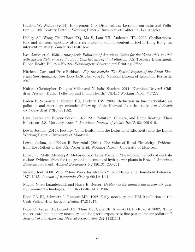
In Table 1, we report the estimates from the difference-in-differences estimation strategy

based on new plant openings. Panel A reports the estimates for all power plants. Across

all three specifications and both control groups the results are positive and statistically

significant, ranging from 0.63 to 2.2. Panel B reports the estimates effects separately for

large and small power plants. The overall effect is driven entirely by the large plants,

consistent with the substantial spike in coal consumption shown in Figure 8. The preferred

estimates imply that the opening of a large power plant is associated with a 2 percent

increase in the local infant mortality rate. In fact, these estimates can be combined with

information on change in coal consumption that occurred following a large plant opening

to derive the impact of power plant coal consumption on infant mortality. The preferred

19The sample includes 75 small power plants that upgraded capacity and crossed the 75mw thresholdwithin 6 years of initial operation. To avoid concerns that coal consumption is endogenous to the timing ofinitial opening, these observations fall under the ‘small’ category in event years in which capacity is below75mw and the ‘large’ category in event years in which capacity is above 75mw.

15

estimates imply that a 1 million ton increase in annual coal consumption is associated with

an increase of (1.03/8.4)×10 = 1.23 in the infant mortality rate. Given that plants were

historically concentrated in densely populated areas, these findings imply substantial health

costs associated with power generation.

5.2 The Impact of Power Plant Coal Consumption and Capacity

on Infant mortality

Table 2 reports the impact of annual variation in power plant coal consumption and

capacity on infant mortality based on equation (2). Columns (1) to (4) report the estimates

of CoalConsct for different specifications. In column (1) we include only year and county

fixed effects, in column (2) we add baseline economic and geographic covariates interacted

with year, in column (3) a state-year fixed effect is included to allow for differential trends

in mortality across states, and column (4) includes the full set of controls.

Panel A of Table 2 reports the results based on all annual variation in coal consumption.

The point estimates range from 0.085 to 0.142 and are all statistically significant. Notably,

the inclusion of economic covariates reduces the magnitude of the point estimates. The

change in the estimate could reflect the fact that changes in coal consumption and industrial

activity were related. Failing to account for the direct impact of industrial pollution on

health would lead to upward-biased estimates.

Panel B reports the results based on coal and hydroelectric capacity. This comparison

provides a useful placebo test, since both sources of electricity should have similar effects on

local economic activity. Across all four specifications, coal-fired capacity is associated with

large statistically significant increases in infant mortality. Meanwhile, the point estimates

for hydro capacity are insignificant and substantially smaller in magnitude. Together these

findings support the research design.

To interpret the magnitude of the effects, Figure 11 reports the additional infant deaths

in the sample that are attributable to coal consumption by electric utilities. We report these

16

estimates separately based on the number of live births in 1938, and based on annual births.

Calculations based on the latter are substantially larger, given that the baby boom led to

an increase in the number of infants potentially exposed to air pollution. In 1938, fewer

than 500 infant deaths can be attributed to coal-fired electricity. As coal-fired generation

expanded in the 1950s, the health costs grew dramatically. By the end of the sample period,

the rise in coal consumption by electric utilities was responsible for an additional 3,500 infant

deaths per year.

5.3 Effects in the Housing Market

Together, the results from Tables 1 and 2 show that local power plant emissions were

harmful for health. These findings are consistent with recent evidence on the effects of local

coal consumption on mortality (Currie et al., 2013; Hanlon, 2014). Nevertheless, it is unclear

how individuals traded-off these health costs against the benefits of local thermal electricity.

To investigate this question, we adopt a hedonic approach, using changes in the housing

market and wages to infer the implicit price associated with this nonmarket amenity. We

estimate the relationship between coal consumption by electric utilities and housing rental

values for decennial years 1940, 1950, and 1960.20

Table 3 presents the estimates of the capitalization of power plant coal-use into property

values. We report the estimates separately for coal consumption and coal-fired capacity

within 30 miles. For reference, columns (1) and (2) report the estimates for infant mortality

based on the same sample used in the housing market regressions. Panel A shows the

estimates for electric utilities coal consumption. Although there were significant negative

effects on health, we find no relationship between coal consumption and property values.

We find similarly small results based on coal-fired capacity. In fact, the substantial increase

in electric utility coal-use between 1940 and 1960 can account for less than 1% percent of

variation in housing prices over this period.

20We focus on rental prices since they are more highly correlated with local amenities than housing prices(Banzhaf and Farooque, 2013).

17

There are several possible explanations for the limited response in the housing or labor

market. First, the findings might simply reflect the fact that individuals were unaware of the

health costs associated with pollution, and thus generally unresponsive to changes in local

coal consumption. Media coverage during this time period did identify the potential risks

associated with pollution, however, epidemiological evidence on the link between pollution

and mortality did not emerge until the 1970s. Alternatively, if there was heterogeneity

in tastes for clean air, individuals may have sorted across locations on the basis of the

unobservable preferences. In this case, our estimates of the marginal willingness to pay

(MWTP) could reflect the preferences of a specific subpopulation that, for example, may

have placed a relatively low value on clean air. Third, the findings may simple capture the

fact that individuals valuations of the benefits associated with local electricity generation

roughly offset the pollution costs. To differentiate amongst these competing explanations,

we exploit heterogeneity in the housing market response.

5.4 Heterogeneous Responses in the Housing Market

To assess heterogeneity in the effects of coal-fired emissions, we split US counties into two

bins according to baseline electricity access.21 We split the sample evenly between these bins,

and re-estimate the effects for infant mortality and housing across the two groups. There

were wide differences in electrification access across the two groups: the mean baseline

electrification rates were 50 and 93 percent for the low and high bins, respectively. This

stark distinction allows us to disentangle the pollution costs from the benefits associated

with electricity access.

Table 4 presents the results for infant mortality and the logarithm of median dwelling

rent. The health effects differ widely according to baseline electricity access. At low levels

of access, increases in coal consumption and coal-fired capacity have negative effects on

infant mortality. These findings are consistent with previous research on the positive health

21Electricity access is proxied by the proportion of homes with electric lighting in the 1940 Census ofHousing

18

effects associated with household electrification (Lewis, 2015, Gohlke 2011). At high levels

of electricity access, the sign of the effect flips, suggesting that the pollution overwhelm any

last marginal gains associated with electricity access.

The last two columns report the estimates for housing values. The insignificant effects

reported in Table 3 mask substantial heterogeneity in the housing market response. At

low levels of electricity access, a 100,000 ton increase in coal consumption would lead to a

2.8 percent rise in local housing values, whereas at high levels of access it would lead to a

decrease of 6.1 percent.

The heterogeneous housing response captures how the tradeoffs of power plant coal con-

sumption evolve as a greater share of the population electrify. At low levels of electricity

access, increases in energy production offer large potential benefits to the local population.

As a greater fraction of the population gain access, the scope for these gains is diminished.

On the other hand, the pollution costs of power generation are generally independent of

electricity access. Individuals will assign more value the amenity benefits associated with

increases in electricity production at low levels of electricity access, and place greater im-

portance on the pollution costs of coal consumption at high levels of access. As a result, the

MWTP to avoid power plant emissions should increase with the level of electricity access,

consistent with the heterogeneity we observe in the hedonic regressions.

The fact that the MWTP to avoid power plant emissions depends on the level of electricity

access has important implications for energy policy. Fossil-fuel generators have long lifespans,

ranging from 30 to 50 years (IEA, 2010). Consider the case of the Gorgas power plant.

This large thermal power plant was built in the late 1920s near the town of Parrish in

Walker County, Alabama. Initially, 70mw of capacity were installed, and the plant consumed

roughly 150,000 tons of coal per year. At the time of installation only 13% of residents had

electrical services. Given these low levels of electricity access, our estimates imply that at

the time of construction of this plant would have caused a 0.3% increase in local home

values, generating a net gain of $379,000 (1990 USD) in the local housing market. By 1950,

19

90% of homes in Walker County had electrical services. As a result, the pollution costs

would have overwhelmed the local benefits of greater electricity access, and led to a 0.9%

fall in local home prices a total decline of $1,653,000 in the value of the county’s housing

stock. Given these large changes in the response of the housing market, policymakers must

take careful account for the evolving preferences for thermal power when investing in energy

infrastructure.

6 Conclusion

This paper uses the sharp expansion in U.S. fossil fuel powered electricity during the

mid-20th century to study the tradeoffs associated with coal-fired power generation. The

analysis draws on newly digitized information on the timing of power plant openings, coal

consumption, and health. Increases in power plant emissions are associated with higher

levels of local pollution and a greater incidence of infant mortality. Although these negative

environmental effects were not considered a disamentity on average, we find substantial

heterogeneity in how individuals valued local thermal capacity. In particular, our estimates

imply a positive MWTP for thermal power at low levels of electricity access, and a negative

MWTP at high levels of access, suggesting that the benefits of electricity may diminish with

economic development.

Our estimates suggest that there was a remarkable reversal in preferences for local ther-

mal electricity during the mid-20th century. In 1925, the construction of a thermal power

plant would have been considered a gain to local residents in the majority of U.S. counties,

and a local disamenity in just 2% of counties. By 1955, fossil fuel power plants were viewed

as a local disamenity in 98% of counties. Perhaps in response to these evolving preferences,

the subsequent fifty years have witnessed increasingly stringent regulations of power plant

emissions under the 1963 Clean Air Act and subsequent amendments. There were sub-

stantial costs associated with meeting these requirements, including costs associated with

20

decommissioning existing plants and upgrading capacity to meet emission standards. Given

these potentially large adjustment costs, policymakers must take into account both current

and future preferences for electricity and air quality when making electricity infrastructure

investment decisions.

References

Almond, Douglas, Yuyu Chen, Michael Greenstone, and Hongbin Li. 2009. “Winter Heatingor Clean Air? Unintended Impacts of China’s Huai River Policy?”, American EconomicReview, 99(2): 184-90.

Arceo-Gomez, Eva, Rema Hanna, and Paulina Oliva. 2012.“Does the Effect of Pollutionon Infant Mortality Differ Between Developing and Developed Countries? Evidence fromMexico City.” NBER Working Paper #18349.

Avery, Christy L., et al. “Estimating error in using ambient PM2. 5 concentrations as proxiesfor personal exposures: a review.” Epidemiology 21.2 (2010): 215-223.

Barreca, Alan, Karen Clay, and Joel Tarr. (2013). “Coal, Smoke, and Death: BituminousCoal and American Home Heating,” NBER Working Paper #19881.

Biondo, S. J., and J. C. Marten. “A History of Flue Gas Desulphurization Systems Since1850.” Journal of the Air Pollution Control Association 27.10 (1977): 948-961.

Chay, Kenneth Y. and Michael Greenstone. 2003a. “The Impact of Air Pollution on InfantMortality: Evidence from Geographic Variation in Pollution Shocks Induced by a Recession.”Quarterly Journal of Economics, 118: 1121-1167.

Chay, Kenneth Y. and Michael Greenstone. 2003a. “Air Quality, Infant Mortality, and theClean Air Act of 1970.” MIT Department of Economics Working Paper No. 04-08.

Chay, Kenneth Y., and Michael Greenstone. “Does Air Quality Matter? Evidence from theHousing Market.” Journal of Political Economy, 113.2 (2005).

Clancy L, Goodman P, Sinclair H, Dockery DW. 2002. “Effect of air-pollution control ondeath rates in Dublin, Ireland: an intervention study.” Lancet 360:12101214.

Clay, Karen and Werner Troesken. 2010. “Smoke and the Rise and Fall of the London Fog” inClimate Change Past and Present. Edited by Gary Libecap and Richard H. Steckel. Chicago:University of Chicago Press, 2010.

Cohen, Aaron et al. 2004. “Chapter 17: Urban Air Pollution” in Comparative Quantificationof Health Risks, Volume 2. Geneva: World Health Organization.

Cropper, Maureen L., and Wallace E. Oates. “Environmental economics: a survey.” Journalof Economic Literature (1992): 675-740.

21

Currie, Janet and Matthew Neidell. 2005. “Air Pollution and Infant Health: What CanWe Learn From California’s Recent Experience?” Quarterly Journal of Economics, 120:1003-1030.

Currie, Janet, Matthew Neidess, Johannes Schmieder. 2009. “Air Pollution and InfantHealth: Lessons from New Jersey.” Journal of Health Economics. 28: 688-703.

Currie, Jarnet and Reed Walker 2011. “Traffic Congestion and Infant Health: Evidence fromE-ZPass.” American Economic Journal: Applied Economics, 3:65-90.

Davidson, C.I., and D.L. Davis. 2005. “A Chronology of Airborne Particulate Matter in Pitts-burgh,” in History and Reviews of Aerosol Science, G.J. Sem, D. Boulard, P. Brimblecombe,D.S. Ensor, J.W. Gentry, J.C.M Marijnissen And O. Preining (Eds.).

DOC (United States Department of Commerce) - Bureau of the Census. (2012). County andCity Data Book [United States] Consolidated File: County Data, 1947-1977. ICPSR07736-v2.Ann Arbor, MI: Inter-university Consortium for Political and Social Research [distributor].

Eisenbud, Merril. 1978. Levels of Exposure to Sulfur Oxides and Particulates in New YorkCity and their Sources. Bulletin of the New York Academy of Medicine 1978, 54:991-1011.

Environmental Protection Agency EPA, AP42. Compilation of Air Pollu-tant Emission Factors, Volume I Stationary Point and Area Sources. (1998).http://www.epa.gov/ttnchie1/ap42/ch01/final/c01s01.pdf.

Environmental Protection Agency. 2000. National Air Pollutant Emission Trends 19001998.US Environmental Protection Agency (2000).

Fishback, Price, Michael Haines, Shawn Kantor, and Joseph Cullen. (s.d.). County and CityMortality Data, 1921 to 1950, available at econ.arizona.edu/faculty/fishback.asp

Gartner, Scott Sigmund, et al. Historical statistics of the United States. Ed. Susan B. Carter.New York: Cambridge University Press, 2006.

Gohlke, Julia M., et al. “Estimating the global public health implications of electricity andcoal consumption.” Environmental health perspectives 119.6 (2011): 821

Goklany, Indur M. Clearing the air: the real story of the war on air pollution. Cato Institute,1999.

Haines, Michael R., and Inter-university Consortium for Political and Social Research(ICPSR). (2010). Historical, Demographic, Economic, and Social Data: The United States,1790-2002. Ann Arbor, MI: Inter-university Consortium for Political and Social Research,icpsr.org.

Hales, Jeremy M. Tall stacks and the atmospheric environment. Environmental ProtectionAgency, Office of Air and Waste Management, Office of Air Quality Planning and Standards,1976.

22

Hanlon, W. Walker. (2014). Endogenous City Disamenities: Lessons from Industrial Pollu-tion in 19th Century Britain, Working Paper - University of California, Los Angeles.

Hedley AJ, Wong CM, Thach TQ, Ma S, Lam TH, Anderson HR. 2002. Cardiorespira-tory and all-cause mortality after restrictions on sulphur content of fuel in Hong Kong: anintervention study. Lancet 360:16461652.

Ives, James et al. 1936. Atmospheric Pollution of American Cities for the Years 1931 to 1933with Special Reference to the Solid Constituents of the Pollution. U.S. Treasury Department,Public Health Bulletin No 224. Washington: Government Printing Office.

Kitchens, Carl, and Price Fishback. Flip the Switch: The Spatial Impact of the Rural Elec-trification Administration 1935-1940. No. w19743. National Bureau of Economic Research,2013.

Knittel, Christopher, Douglas Miller and Nicholas Sanders. 2011. “Caution, Drivers! Chil-dren Present. Traffic, Pollution and Infant Health.” NBER Working Paper #17222.

Laden F, Schwartz J, Speizer FE, Dockery DW. 2006. Reduction in fine particulate airpollution and mortality: extended follow-up of the Harvard six cities study. Am J RespirCrit Care Med 173(6):581582.

Lave, Lester and Eugene Seskin. 1972. “Air Pollution, Climate, and Home Heating: TheirEffects on U.S. Mortality Rates.” American Journal of Public Health 62: 909-916.

Lewis, Joshua. (2014). Fertility, Child Health, and the Diffusion of Electricity into the Home,Working Paper - University of Montreal.

Lewis, Joshua, and Edson R. Severnini. (2014). The Value of Rural Electricity: Evidencefrom the Rollout of the U.S. Power Grid, Working Paper - University of Montreal.

Lipscomb, Molly, Mushfiq A. Mobarak, and Tania Barham. “Development effects of electrifi-cation: Evidence from the topographic placement of hydropower plants in Brazil.” AmericanEconomic Journal: Applied Economics 5.2 (2013): 200-231.

Mokyr, Joel. 2000. Why “More Work for Mothers?” Knowledge and Household Behavior,1870-1945, Journal of Economic History 60(1): 1-41.

Nagda, Niren Laxmichand, and Harry E. Rector. Guidelines for monitoring indoor air qual-ity. Geomet Technologies, Inc., Rockville, MD, 1986.

Pope CA III, Schwartz J, Ransom MR. 1992. Daily mortality and PM10 pollution in theUtah Valley. Arch Environ Health. 47:211217.

Pope, C. Arden, III, Burnett RT, Thun MJ, Calle EE, Krewski D, Ito K, et al. 2002, “Lungcancer, cardiopulmonary mortality, and long-term exposure to fine particulate air pollution.”Journal of the American Medical Association. 287:11321141.

23

Pope, C. Arden, III, Douglas L. Rodermund, and Matthew M. Gee. 2007. “Mortality Effectsof a Copper Smelter Strike and Reduced Ambient Sulfate Particulate Matter Air Pollution.”Environmental Health Perspectives. 115(5): 679683.

Ridker, Ronald G., and John A. Henning. “The Determinants of Residential Property Valueswith Special Reference to Air Pollution,” The Review of Economics and Statistics (1967):246-257.

Stern, Arthur C. “History of Air Pollution Legislation in the United States.” Journal of theAir Pollution Control Association 32.1 (1982): 44-61.

U.S. Federal Power Commission. (1947). Steam-Electric Plant Construction Cost and AnnualProduction Expenses, 1938-1947. Washington DC: U.S. Federal Power Commission.

U.S. Federal Power Commission. (1948-62). Steam-Electric Plant Construction Cost andAnnual Production Expenses (Annual Supplements). Washington DC: U.S. Federal PowerCommission.

U.S. Federal Power Commission. (1963). Principal Electric Power Facilities in the UnitedStates (map). Washington DC: U.S. Federal Power Commission.

United States Bureau of the Census. Historical statistics of the United States, colonial timesto 1970. No. 93. US Department of Commerce, Bureau of the Census, 1975.

United States Bureau of Mines. Minerals Yearbook (various years). Washington: GovernmentPrinting Office.

United States Department of Health, Education and Welfare 1958. Air Pollution Measure-ments of the National Air Sampling Network: Analyses of Suspended Particulates, 1953-1957. Public Health Service Publication No 637. Washington: Government Printing Office.

United States General Accountability Office. 2012, Air Emissions and Electric-ity Generation at U.S. Power Plants. Washington: Government Printing Office.http://gao.gov/assets/600/590188.pdf.

Woodruff, Tracey, Lyndsey Darrow, and Jennifer Parker. 2008. “Air Pollution and Post-neonatal Infant Mortality in the United States, 1999-2002.” Environmental Health Perspec-tives 116: 110-115.

24

7 Figures and Tables

Table 1: The Effect of Power Plant Openings on Infant MortalityDep Variable: Infant Mortality

Sample selection:<60 miles from a plant <90 miles from a plant

(1) (2) (3) (4) (5) (6)Panel A: All Power Plants

I(PP open)× Near 2.2051** 1.5159*** 0.6477* 1.9541* 1.4091*** 0.6255**(1.1212) (0.5006) (0.3440) (1.0053) (0.4827) (0.2704)

Panel B: Large vs. Small Power Plants

I(PP open)× Near×Large PP 2.4333** 1.8707*** 1.0393*** 2.1541** 1.7604*** 1.0300***

(1.1893) (0.5044) (0.3630) (1.0613) (0.4898) (0.2969)

Small PP 1.0972 -0.0590 -0.3929 0.8940 -0.2380 -0.4453(0.8190) (0.5658) (0.4354) (0.7351) (0.5054) (0.3613)

Observations 69,650 69,650 69,650 141,300 141,300 141,300# Plants 267 267 267 281 281 281

ControlsYear+County-plant FE Y Y Y Y Y YState-year FE Y Y Y YGeog & econ × year Y Y

25

Table 2: The effect of power plant coal consumption and capacity on infant mortalityDep Variable: Infant Mortality

(1) (2) (3) (4)Panel A: Coal Consumption Within 30 Miles

Coal Consumption Within 30 Miles 0.1418*** 0.0897*** 0.1082*** 0.0850***(0.0357) (0.0257) (0.0194) (0.0167)

Panel B: Coal Capacity vs. Hydro Capacity

Coal Capacity Within 30 Miles 0.0022*** 0.0018*** 0.0019*** 0.0016***(0.0005) (0.0004) (0.0003) (0.0003)

Hydro Capacity Within 30 Miles -0.0013 0.0005 0.0004 -0.0003(0.0026) (0.0013) (0.0012) (0.0014)

Counties 1,983 1,983 1,983 1,983Observations 49,575 49,575 49,575 49,575

ControlsCounty & Year FE Y Y Y YState-Year FE Y YGeog & economic covariates Y Y

26

Table 3: The effect of power plant coal consumption and capacity on property valuesInfant Mortality Ln(Median Rent)

(1) (2) (3) (4)Panel A: Coal Consumption Within 30 Miles

CC30Miles 0.1288* 0.1010** -0.0021 0.0011(0.0658) (0.0465) (0.0015) (0.0009)

Panel B: Coal Capacity Within 30 Miles

Cap30Miles 0.2391*** 0.2650*** -0.0083*** 0.0000(0.0652) (0.0691) (0.0025) (0.0019)

Counties 1,983 1,983 1,983 1,983Observations 49,575 49,575 49,575 49,575

ControlsCounty & Year FE Y Y Y YAll covariates Y Y

27

Table 4: Heterogeneity in the effects on property values, by baseline electricity accessInfant Mortality Ln(Median Rent)(1) (2) (3) (4)

Panel A: Coal Consumption Within 30 Miles

CC30Miles x L-Electricity -0.2169*** -0.1760*** 0.0032*** 0.0028***-0.0678 -0.061 -0.0009 -0.0008

CC30Miles x H-Electricity 0.2411*** 0.2487*** -0.0204*** -0.0061**-0.0709 -0.0546 -0.0042 -0.0024

Panel B: Coal Capacity Within 30 Miles

Cap30Miles x L-Electricity -0.5817*** -0.4108** 0.0085*** 0.0064***(0.1893) (0.1634) (0.0024) (0.0022)

Cap30Miles x H-Electricity 0.2976*** 0.3701*** -0.0247*** -0.0086***(0.0652) (0.0768) (0.0043) (0.0028)

ControlsCounty & Year FE Y Y Y YAll covariates Y Y

28

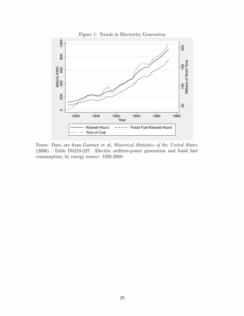
Figure 1: Trends in Electricity Generation

5010

015

020

0M

illion

s of

Sho

rt To

ns

020

040

060

080

010

00Bi

llions

KW

H

1940 1945 1950 1955 1960 1965Year

Kilowatt Hours Fossil Fuel Kilowatt HoursTons of Coal

Notes: Data are from Gartner et al, Historical Statistics of the United States(2006). Table Db218-227. Electric utilities-power generation and fossil fuelconsumption, by energy source: 1920-2000.

29

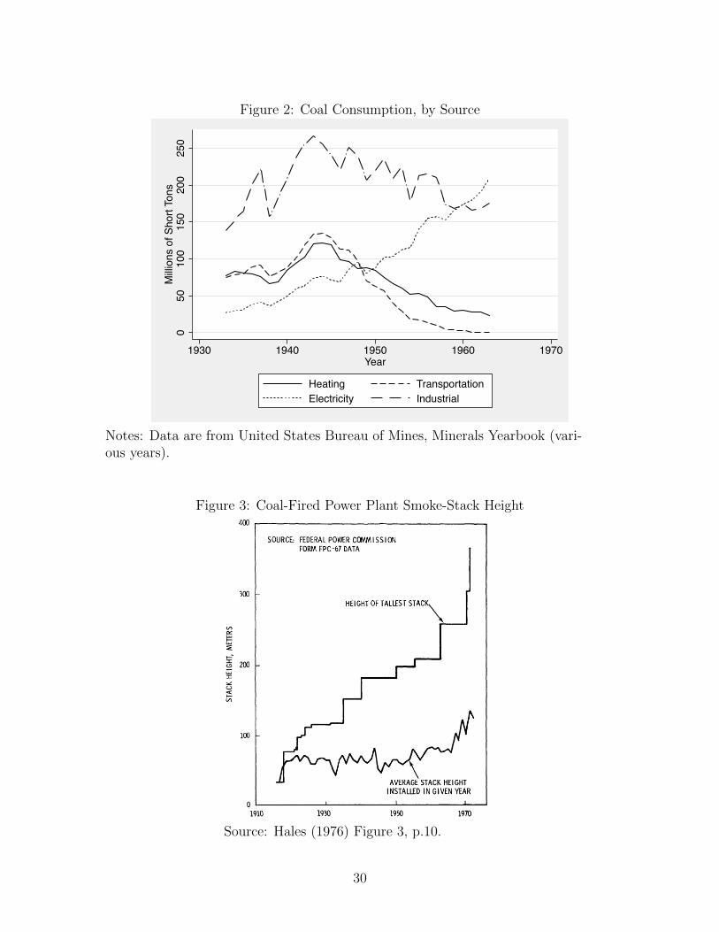
Figure 2: Coal Consumption, by Source

050

100

150

200

250

Milli

ons

of S

hort

Tons

1930 1940 1950 1960 1970Year

Heating TransportationElectricity Industrial

Notes: Data are from United States Bureau of Mines, Minerals Yearbook (vari-ous years).

Figure 3: Coal-Fired Power Plant Smoke-Stack Height

Source: Hales (1976) Figure 3, p.10.

30

Figure 4: Distribution of Fossil-Fuel Capacity

Den

sity

25 50 75 100 125 150 175 200Distance to City Center (Miles)

Power Plant Capacity (1930)Power Plant Capacity (1960)

Notes: This figure report the density of fossil-fuel capacity within 200 miles ofthecity-centroid for the 50 largest cities in the US.

Figure 5: Dispersion of PM2.5 Around Large Power Plants

Treatment counties← → Control counties← →Control counties← →

05

1015

20%

of P

M2.

5 Exp

osur

e

0 30 60 90 120 150Distance to Power Plant (miles)

TSP Exposure TSP Exposure (per area of land)

Source: Levy et al (2002)

31

Figure 6: Impact of Large Power Plants on Electricity Access

Treatment counties← → Control counties← →Control counties← →

02

46

810

% H

omes

with

Ele

ctric

ity

0 30 60 90 120 150Distance to Power Plant (miles)

Effect of Power Plant Opening 95% C.I.

Notes: This figure plots the regression estimates from FE models relating frac-tionof households with electricity to opening of large power plants (>30mw)

32

Figure 7: Event Study for the Effect of Power Plant Openings on Infant Mortality

Construction

-.50

.51

1.5

Infa

nt M

orta

lity R

ate

Per 1

000

Live

Birt

hs

-6 -5 -4 -3 -2 -1 0 1 2 3 4 5 6Years Relative to Power Plant Opening

Notes: This figure plots the coefficient estimates for t ∈ {−6, 6} based on equa-tion (1).

Figure 8: Coal Consumption for Large and Small Power Plants

0

1

2

3

4

5

6

7

8

9

10

Coal

Con

sum

ptio

n (1

00,0

00 to

ns)

-6 -5 -4 -3 -2 -1 0 1 2 3 4 5 6Years Relative to Power Plant Openings

Plants Size >75MW Plants Size <75MW

Notes: This figure plots average annual coal consumption (100,000s tons)for large (>75mw) and small (<75mw) following opening.

33

Figure 9: Impact of Large Power Plant Openings on Infant Mortality

Construction

-.50

.51

1.5

Infa

nt M

orta

lity R

ate

Per 1

000

Live

Birt

hs

-6 -5 -4 -3 -2 -1 0 1 2 3 4 5 6Years Relative to Power Plant Opening

Notes: This figure plots the coefficient estimates for t ∈ {−6, 6} based on equa-tion (1) for large power plants (>75mw).

Figure 10: Impact of Small Power Plant Openings on Infant Mortality

Construction

-1.5

-1-.5

0.5

1In

fant

Mor

tality

Rat

e Pe

r 100

0 Li

ve B

irths

-6 -5 -4 -3 -2 -1 0 1 2 3 4 5 6Years Relative to Power Plant Opening

Notes: This figure plots the coefficient estimates for t ∈ {−6, 6} based on equa-tion (1) for small power plants (<75mw).

34

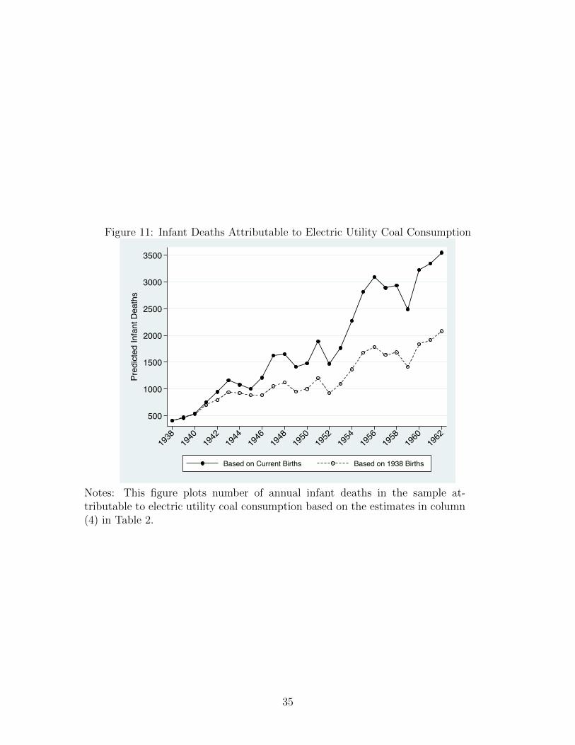
Figure 11: Infant Deaths Attributable to Electric Utility Coal Consumption

500

1000

1500

2000

2500

3000

3500

Pred

icte

d In

fant

Dea

ths

1938

1940

1942

1944

1946

1948

1950

1952

1954

1956

1958

1960

1962

Based on Current Births Based on 1938 Births

Notes: This figure plots number of annual infant deaths in the sample at-tributable to electric utility coal consumption based on the estimates in column(4) in Table 2.

35

A Appendix

A.1 Additional Figures and Tables

Table A.1: TSP Concentration in Various YearsLocation Time TSP SourceChicago 1912-1913 760 Eisenbud (1978)14 Large US Cities 1931-1933, Winter 510 Ives et al (1936)US Urban Stations 1953-1957 163 U.S. Department of Health, Education and Welfare (1958)8 of 14 Large US Cities 1954 214 U.S. Department of Health, Education and Welfare (1958)US Urban Stations 1960 118 Lave and Seskin (1972)14 Large US Cities 1960 143 EPA data

US National Average 1990 60 Chay and Greenstone (2003a)58 Chinese Cities 1980-1993 538 Almond et al (2009)Worldwide 1999 18% of urban pop > 240 Cohen et al (2004)

Notes: The original measurements were in TSP for all of the sources except for Cohen et al (2004). Cohen et al, Figure 17.3 (World), indicates that 18% of the urban population lived in locations where the PM10 was greaterthan 100. We translated the PM10 values to TSP using the following formula: PM10/0.417, where 0.417 is theempirical ratio of PM10 to TSP in their world data (Table 17.4). The estimate for 1990 is from Chay andGreenstone (2003a), Figure 1. EPA data are authors calculations based on EPA dataset for 1960.

Table A.2: Municipal Smoke Abatement Legislation Prior to 1930Decade Cities Passing Legislation1880-1890 Chicago, Cincinnati

1890-1900 Cleveland, Pittsburgh, St. Paul

1900-1910 Akron, Baltimore, Boston, Buffalo, Dayton, Detroit, Indianapolis, Los Angeles, Milwaukee, Minneapolis,New York, Newark, Philadelphia, Rochester, St. Louis, Springfield (MA), Syracuse, Washington

1910-1920 Albany County (NY), Atlanta, Birmingham, Columbus, Denver, Des Moines, Duluth, Flint, Hartford, Jersey City,Kansas City, Louisville, Lowell, Nashville, Portland (OR), Providence, Richmond, Toledo

1920-1930 Cedar Rapids, East Cleveland, Erie County (NY), Harrisburg, Grand Rapids, Lansing, Omaha,Salt Lake City, San Francisco, Seattle, Sioux City, Wheeling

Source: Stern 1982, Table III, p. 45.

36