Can Bias Correction of Regional Climate Model Lateral BoundaryConditions Improve Low-Frequency Rainfall Variability?

EYTAN ROCHETA

School of Civil and Environmental Engineering, University of New South Wales, Sydney,

New South Wales, Australia

JASON P. EVANS

Climate Change Research Centre, and ARC Centre of Excellence for Climate System Science, University of

New South Wales, Sydney, New South Wales, Australia

ASHISH SHARMA

School of Civil and Environmental Engineering, University of New South Wales, Sydney,

New South Wales, Australia

(Manuscript received 31 August 2016, in final form 5 July 2017)

ABSTRACT

Global climate model simulations inherently contain multiple biases that, when used as boundary condi-

tions for regional climate models, have the potential to produce poor downscaled simulations. Removing

these biases before downscaling can potentially improve regional climate change impact assessment. In

particular, reducing the low-frequency variability biases in atmospheric variables as well as modeled rainfall is

important for hydrological impact assessment, predominantly for the improved simulation of floods and

droughts. The impact of this bias in the lateral boundary conditions driving the dynamical downscaling has not

been explored before. Here the use of three approaches for correcting the lateral boundary biases including

mean, variance, and modification of sample moments through the use of a nested bias correction (NBC)

method that corrects for low-frequency variability bias is investigated. These corrections are implemented at

the 6-hourly time scale on the global climate model simulations to drive a regional climate model over the

Australian Coordinated Regional Climate Downscaling Experiment (CORDEX) domain. The results show

that the most substantial improvement in low-frequency variability after bias correction is obtained from

modifying the mean field, with smaller changes attributed to the variance. Explicitly modifying monthly and

annual lag-1 autocorrelations through NBC does not substantially improve low-frequency variability attri-

butes of simulated precipitation in the regional model over a simpler mean bias correction. These results raise

questions about the nature of bias correction techniques that are required to successfully gain improvement in

regional climate model simulations and show that more complicated techniques do not necessarily lead to

more skillful simulation.

1. Introduction

Climate change impact assessment can use regional

climate models (RCMs) to provide higher-resolution

projections than available from global climate models

(GCMs). RCMs are driven by large-scale circulation

patterns from the GCM being transferred through lateral

boundary conditions (LBCs), as well as specified initial

conditions and lower boundaries. As these models are

driven by coarse-scale GCM data, they are dependent on

the provision of realistic simulations of the global climate

to serve as their lateral boundaries.

There is a range of literature associated with biases in

GCMs, including bias in the sea surface temperature

(Bruyère et al. 2014), wind fields (Capps and Zender

2008), specific humidity (John and Soden 2007), atmo-

spheric variables in CMIP3 (van Ulden and van

Oldenborgh 2006; Vial and Osborn 2012) and CMIP5

(Brands et al. 2013; Jury et al. 2015), and the low-

frequency variability of precipitation (Rocheta et al.

2014a). These GCM biases result from poorly un-

derstood physical processes, model resolution, andCorresponding author: A. Sharma, a.sharma@unsw.edu.au

VOLUME 30 J OURNAL OF CL IMATE 15 DECEMBER 2017

DOI: 10.1175/JCLI-D-16-0654.1

� 2017 American Meteorological Society. For information regarding reuse of this content and general copyright information, consult the AMS CopyrightPolicy (www.ametsoc.org/PUBSReuseLicenses).

9785

numerical parameterizations within the GCM. While

reduced when aggregated over continental spatial or

yearly time scales, they result in biases in the RCM

simulations to which they provide input. Many studies

have shown that improper boundary conditions will af-

fect the entire limited-area RCM domain (Caldwell

et al. 2009; Rojas and Seth 2003; Warner et al. 1997; Wu

et al. 2005).

A common approach to deriving useful atmospheric

variables for impact studies involves performing bias

correction on RCM output (Casanueva et al. 2016; Kim

et al. 2015, 2016; Ruiz-Ramos et al. 2016; Teutschbein

and Seibert 2012). This requires observational datasets

at the spatial and temporal resolution of the RCM out-

put, which is often not available. Most bias correction

techniques do not maintain intervariable relationships

that may be important for driving subsequent impact

models (see Rocheta et al. 2014b; Ehret et al. 2012).

However, some new approaches are attempting more

sophisticated multivariable bias correction methods

such as the Inter-Sectoral Impact Model Intercomparison

(ISI-MIP) method (Hempel et al. 2013) and the em-

pirical copula–bias correction method (Vrac and

Friederichs 2015).

The question of whether correcting these biases in the

RCM input improves the quality of the RCM simulated

outputs is one that has only started to be investigated in

detail. For example, Holland et al. (2010) show im-

provement of the RCM simulation of tropical cyclones

using a linear bias correction on the forcing GCM data.

Colette et al. (2012) use a quantile–quantile (QQ)-based

correction on the input data to improve RCM simula-

tions of European temperature and precipitation.

Bruyère et al. (2014) addressed climatological mean

corrections in an attempt to improve hurricane simula-

tions, Xu and Yang (2012) applied mean and variance

corrections in an attempt to improve model output, and

White and Toumi (2013) compared linear and QQ ap-

proaches. Meyer and Jin (2016) attempted to produce a

physically consistent bias correction by making use of

the physical relationships underpinning the climate

models. They did this through bias correcting three

variables from which the others could be derived. The

results from these studies have varied but generally

found an improvement after correcting mean fields with

lesser improvement through more complex correction

approaches.

An issue that has not been studied is whether the

correction of low-frequency variability, or interannual

variability, biases in GCM simulations leads to a better

simulation of similar variability in RCM rainfall, which

is of practical interest in hydrology, and the focus of this

study. As such, not only are we interested in correcting

the distributional attributes of the GCM simulations,

but we are also interested in correcting lag-1 autocor-

relation attributes at multiple temporal scales to make

sure the LBCs driving the higher-resolution simulation

have the most realistic characteristics possible. We ap-

proach this investigation using an RCM simulation

without any correction, followed by a range of bias

corrections on the LBCs, to assess the changes that re-

sult in the ensuing rainfall fields. This studymakes use of

CMIP3 output downscaled using the Weather Research

and Forecasting model over the Australasian Co-

ordinated Regional Climate Downscaling Experiment

(CORDEX) domain.

This paper is laid out as follows. The next section

details the methods involved in this work, including

the various bias correction techniques, metrics for

measuring bias correction performance, and the datasets

used. The results are then presented in section 3. Finally,

a discussion that identifies the main limitations of

this work and presents overall conclusions completes

this paper.

2. Methods

a. Models and data

The GCM used in this study was the Commonwealth

Scientific and Industrial Research Organization’s Mk3.5

simulation of historical climate made available by the

World Climate Research Program (WCRP) Coupled

Model Intercomparison Project phase 3 (CMIP3)

(Meehl et al. 2007). The CSIROGCM is a fully coupled

climate model on 18 hybrid-sigma vertical levels and

T63 Gaussian grid (~1.8758 latitude3 1.8758 longitude).It has been successfully used to drive RCM simulations

in Australia (Evans and McCabe 2013).

The reanalysis model used as an ‘‘observational’’

reference for bias correction was the European Center

for Medium-Range Weather Forecast’s (ECMWF)

ERA-Interim (ERA-I hereinafter) reanalysis (Dee

et al. 2011) on 0.758 latitude3 0.758 longitude resolutionwith 60 model levels from the surface up to 0.1 hPa. This

model was integrated through the RCM to produce the

ERA-I-driven WRF baseline simulation, a ‘‘best-case’’

or ‘‘ideal’’ regional climate simulation against which the

bias corrected cases are compared.

For the purpose of bias correction, ERA-I variables of

zonal winds u, meridional winds y, temperature T, and

specific humidity q were regridded to align with

CSIRO’s resolution for 31 yr from 1 January 1980 to

31 December 2010. Initial conditions, such as soil

moisture, soil temperature, snow depth, leaf area index,

etc., were not corrected and remained identical in each

9786 JOURNAL OF CL IMATE VOLUME 30

simulation. The lower boundary condition of sea sur-

face temperature (SST) was regridded in the same

way as the atmospheric variables. Sea ice was not in-

cluded as it is not present in the given domain. The

listed variables are the only atmospheric and primary

surface variables taken from a global model and in-

gested into the RCM through the LBCs and lower

boundaries respectively.

The Weather Research and Forecasting (WRF)

Model with dynamical core, version 3.3 (Skamarock

et al. 2008) was the RCM used in this study. The RCM

grid resolution, shown in Fig. 1, was ;50km with 30

vertical eta levels, and an atmosphere pressure top of

0.5 hPa, spanning the Australasian CORDEX domain

(http://www.cordex.org/community/domain-australasia-

cordex.html) with dimensions of 144 3 215 horizontal

grid points. The curvilinear rotated latitude–longitude

projection is used as the model horizontal coordinate.

TheWRFModel simulation usesMellor–Yamada–Janjic

planetary boundary layer (Janjic 1994),Betts–Miller–Janjic

cumulus scheme (Janjic 1994), WRF double-moment

5-class microphysics (Lim and Hong 2010), RRTM

longwave radiation (Mlawer et al. 1997), Dudhia

shortwave radiation (Dudhia 1989), and unified Noah

land surface model (Tewari et al. 2004). This setup has

been demonstrated by Evans et al. (2012) and Olson

et al. (2016) to simulate reliably over the domain. The

simulations were integrated from 0006 UTC 1 January

1980 to 0000 UTC 1 January 2011. The first year was

excluded to remove all issues associated with spinup and

to produce a full 30-yr simulation.

The Australian Water Availability Project (AWAP)

rainfall product (Jones et al. 2009) is a gridded analysis

dataset based on observations and was used in con-

junction with the ERA-I-driven WRF data to validate

the simulations of rainfall over the Australian landmass.

These data, originally of 0.058 latitude and longitude

(~5km 3 5 km) resolution, were regridded to the same

resolution and projection of the RCM simulations. The

same time span as the WRF Model output was used in

the evaluation study.

b. Bias correction techniques

As mentioned earlier, numerous studies have identi-

fied a wide range of biases in GCM fields compared to

observations. Of particular importance in this paper are

biases associated with rainfall that lead to sustained

anomalies, namely characteristics of persistence (the

sequence of sustained high or low rainfalls) or long-term

variability (Johnson et al. 2011). To address any im-

provement in the RCM simulation from bias correction

techniques we applied three techniques that corrected

different aspects of a variable’s statistical distribution

with increasing complexity. Similar to Bruyère et al.

(2014), Colette et al. (2012), and Xu and Yang (2012),

these corrections are applied to variables used in the

lateral and lower boundary conditions: temperature,

water vapor, winds, and SST. What is different with the

FIG. 1. Regional domain (Australasian CORDEX domain) used for all RCM simulations.

Shading represents terrain height (m) and the red lines shows the edge of the relaxation zone.

15 DECEMBER 2017 ROCHETA ET AL . 9787

approach taken here from the literature mentioned

above is that corrections were applied to 6-hourly GCM

data in monthly or annual groups, instead of a single

climatological correction on the whole dataset. This

means that for a monthly correction there are 12 cor-

rection factors (i.e., one correction factor for all Janu-

aries, another for all Februaries, etc.) This approach

allows correction for the gross biases in the monthly and

annual data while maintaining sub-month variability.

This approach also allows for more complex techniques

where different corrections are applied to each group of

months or years and corrections can be nested via the

nested bias correction discussed below. All bias correc-

tion approaches were conducted on the entire 31-yr

global dataset. A summary of the bias correction ap-

proaches used in this paper is presented in Table 1.

Generalized advantages and limitations as well as ref-

erences are also given.

1) SIMPLE BIAS CORRECTION

Monthly mean corrections were applied to give cor-

rections on the mean field for each cell and variable

only, without modifying any other aspect of the distri-

bution. This correction, while very simple, improves the

mean atmospheric state and has been shown to provide

improvement in the RCM simulation [e.g., Xu and Yang

(2012), where a climatological correction was applied].

The correction was applied by calculating 12 monthly

means from both GCM and observations and then cor-

recting each variable individually at each time step using

the following formula:

X 0hrly 5 (X

hrly2X)1Y , (1)

where X 0hrly is the corrected GCM variable, Xhrly is the

original GCM variable, andX andY are the GCM’s and

observations’ respective monthly variable means.

2) VARIANCE BIAS CORRECTION

To improve the representation of variance within the

simulation, a standard deviation correction was added to

the simple bias correction approach [Eq. (1)] and ap-

plied as follows:

X 0hrly 5

(Xhrly

2X)

sX

sY1Y , (2)

where sX and sY are the monthly standard deviations of

the GCM and observation variables, respectively. All

variables were corrected additively for the mean and

multiplicatively for variance. After corrections, all var-

iables were subjected to limiting bounds to ensure they

were within a reasonable physical range of the observed

variables. It should be noted that the standard de-

viations above are estimated at the raw 6-hourly time

scale of the simulation, separately for each month of the

year, calculating submonthly variance for 372 months

(31 yr).

3) LOW-FREQUENCY VARIABILITY BIAS

CORRECTION

To improve the representation of low-frequency var-

iability in the RCM simulation, a nested bias correction

(NBC) was applied. This correction acts in a similar way

TABLE 1. Comparison of bias correction techniques used in this study.

Bias correction technique Abbrev. Advantages Limitations Selected references

Uncorrected GCM GCM Physically consistent variable

relationships.

Variables contain biases. —

Mean on atmosphere

and SST

GCMx Ease of application. Limited improvement in

hydrologically relevant

statistical attributes.

Variable relationships

not physically consistent.

(Bruyère et al. 2014;

Ratnam et al. 2016)

Mean and standard

deviation on atmosphere

and SST

GCMx,s Simple application similar

to mean correction,

improves two statistical

moments.

Does not attempt to correct

lag-1 autocorrelation

attributes. Variable

relationships not

physically consistent.

Xu and Yang (2012)

without SST

correction

NBC on atmosphere

and SST

GCMNBC Applies corrections on

multiple ‘‘nested’’ time

scales. Modifies lag-1

autocorrelation attributes

through a transfer function.

Complexity and model

assumptions. Variable

relationships not

physically consistent.

(Johnson and Sharma

2011; 2012; Rocheta

et al. 2014a)

NBC on atmosphere with

original GCM SST

GCMNBC-noSST Used to determine impact

of SST in RCM.

SST and atmospheric

fields inconsistent.

—

9788 JOURNAL OF CL IMATE VOLUME 30

to the above corrections, modifying both the mean and

standard deviations, but adds a model to transfer lag-1

autocorrelation attributes between GCM and reanalysis

models. As 12 monthly correction factors are applied

(i.e., for all Januaries, all Februaries, etc.,) modifying the

lag-1 attributes has an effect, even with monthly mean

and standard deviation corrections. In addition, the

technique allows for multiple nested time scales to be

corrected sequentially. Nested bias correction was un-

dertaken along the lines of Johnson and Sharma (2012)

andMehrotra and Sharma (2012) and has been shown to

improve low-frequency variability attributes in rainfall

(Mehrotra and Sharma 2012; Rocheta et al. 2014a).

NBC is performed through first standardizing the

smallest aggregated time series (monthly in this case) to

remove the model sample mean and standard de-

viations. Standardization is done by first subtracting the

model mean and dividing by the model standard de-

viation. Then the lag-1 autocorrelations are removed

from the standardized time series and are replaced by

the observed monthly lag-1 autocorrelations using the

transfer function:

x0 5 robsi xi21

1ffiffiffiffiffiffiffiffiffiffiffiffiffiffiffiffiffiffiffiffiffi12 (robsi )2

q 264x

i2 rGCM

i xi21ffiffiffiffiffiffiffiffiffiffiffiffiffiffiffiffiffiffiffiffiffiffiffiffi

12 (rGCMi )2

q375, (3)

where x0 is the corrected GCM variable, robsi is the ob-

served lag-1 autocorrelation, and rGCMi is the lag-1 au-

tocorrelation in the GCM variable for time step i.

This new monthly time series is then multiplied by the

observed standard deviation and the observed mean is

added to derive the corrected monthly time series X 0mon.

Note that the lowercase representation in Eq. (3)

denotes a standardized series to distinguish from the

rescaled series, which is denoted in upper case (X 0).These monthly values are aggregated to an annual scale

before the process is repeated. This results in four time

series that are used in Eq. (4) to correct the raw GCM

6-hourly time series Xhrly to produce the corrected time

series X 0hrly: the uncorrected monthly time series Xmon,

the corrected monthly time seriesX 0mon, the uncorrected

annual time series Xann, and the corrected annual time

series X 0ann:

X 0hrly 5

�X 0

mon

Xmon

��X 0

ann

Xann

�X

hrly. (4)

Unlike the previous two bias correction techniques

where correction was applied to all input data (LBCs

and lower boundaries), NBC was applied to the data-

set in two ways: 1) GCMNBC where all input data

were corrected and 2) GCMNBC-noSST where NBC was

applied only to the LBCs with no correction applied to

the SST (i.e., original CSIRO SST is used). This last case

helps to identify the influence of correcting low-frequency

variability attributes of the SSTs over the domain.

c. Performance assessment

To quantify the impact of bias correction on the var-

ious attributes of the variable distributions we have used

qualitative scatterplots with two quantitative measures:

root-mean-square deviation (RMSD) and the aggre-

gated persistence score (APS). RMSD analysis is per-

formed on the entire time series of the bias-corrected

data as well as used to compare the RCM simulations

against ERA-I-driven WRF and AWAP observations.

The APS is used to compare rainfall attributes of the

various RCM simulations.

The first measure, RMSD, is used extensively to

quantify the overall predictive power of the models

compared to observations. The RMSD of predicted

values xi for times t compared to a dependent variable xifor n different predictions is calculated as the square

root of the mean of the squares of the deviations:

RMSD5

ffiffiffiffiffiffiffiffiffiffiffiffiffiffiffiffiffiffiffiffiffiffi�n

t5i

(xi2 x

i)2

n

vuuut. (5)

In addition to using RMSD to show changes in the

different bias correction approaches, we used the ag-

gregated persistence score, which identifies changes in

low-frequency variability attributes (Rocheta et al.

2014a) in rainfall. This measure is based on the premise

that a dataset with low-frequency variability charac-

teristics, when aggregated to increasingly longer ag-

gregation periods, will produce greater variance than a

dataset without low-frequency variability. In this case,

monthly and annual aggregation periods were used.

The APS is a comparative measure of two rainfall

datasets and full details of the APS formulation can be

found in Rocheta et al. (2014a) with only a summary

provided here. The APS is calculated in two steps: the

first calculation quantifies differences in standard de-

viation at each aggregation period divided by a scaling

factor, and the second component calculates the APS

through averaging these differences over the aggrega-

tion periods. Equations (6) and (7) show these re-

spective steps:

SDa5

s(a)sim

2s(a)obs

Ba

, (6)

APS51

a�a

SDa, (7)

15 DECEMBER 2017 ROCHETA ET AL . 9789

where SDa is deemed the scaled deviance at aggregation

a, s(a) is the standard deviation of the ath aggregation

period for both simulation and observation, and Ba is

the reference no-persistence confidence interval of the

standard deviation for the same aggregation period a.

This no-persistence confidence interval is derived by

bootstrapping observations without replacement from

12 monthly bins containing each month’s data points.

This leads to a randomized time series maintaining

seasonal variability while removing all interannual var-

iability. The term Ba is then calculated as the 90%

confidence interval for each a. This APS metric

provides a value of the overall performance of the

comparison of the SDa values between the GCM and

observations for each grid cell. For each cell a positive

(or negative) APS indicates the persistence attributes of

theGCMare larger (smaller) than the observations with

equal persistence attributes identified with APS values

of zero.

In summary, the work presented here follows this

method. 1) Bias correct GCM atmospheric and surface

variables using ERA-I as reference to generate GCMx,

GCMx,s, GCMNBC, and GCMNBC-noSST. All atmo-

spheric and surface variables used as WRF boundary

inputs are corrected. 2) IntegrateWRFwith and without

applied corrections as well as ERA-I case to generate

the six WRF simulations: RCM(ERA-I), RCM(GCM),

RCM(GCMx), RCM(GCMx,s), RCM(GCMNBC), and

RCM(GCMNBC-noSST). 3) Finally, evaluate RCM at-

mospheric and surface variables against RCM(ERA-I)

and AWAP observations.

3. Results

The results are separated into two sections: Sections

3a and 3b evaluate the statistics of the bias-corrected

simulations over the Australasian CORDEX domain

with respect to the ERA-I and ERA-I-driven WRF

datasets respectively. These comparisons reveal the ef-

fectiveness of bias correction of the boundaries of the

RCM (section 3a) as well as the RCM simulation (sec-

tion 3b). Sections 3c and 3d then evaluate the rainfall

statistics over the Australian landmass with regard to

AWAP observations and ERA-I-driven WRF gener-

ated rainfall.

a. Evaluation of bias-corrected GCM data

In this section we evaluate the influence of bias cor-

rection on the global data that have been subsetted to

contain the Australasian CORDEX domain.

The atmospheric and surface variables (u, y, T, q, and

SST) were corrected in the three ways outlined in

section 2b. Figure 2 shows a scatterplot comparing each

correction to ERA-I for specific humidity q. This figure

shows the effect of the different bias correction methods

(rows) over several statistics presented in monthly and

annual aggregations (columns). Each point represents a

3D grid cell within the domain. The monthly statistics

show a separate point for each month and year, whereas

the annualized plots show a single point for each year;

hence there are 12 times as many points in the monthly

plots. It is clear that without correction (Fig. 2a) the raw

GCM simulation contains a spread of values differing

from ERA-I in all statistics. It is particularly scattered

for monthly standard deviation and monthly lag-1 au-

tocorrelation as well as for annual lag-1 autocorrelation.

This spread is relatively uniform for most statistics and

does not contain an overwhelming systematic high or

low bias over all the data. Systematic biases related to

individual months, vertical levels, or regions may reveal

useful information about where to target bias correction

but were not assessed here. The annual mean of specific

humidity corresponds well with ERA-I, indicating the

GCM’s reasonable nature when looking at annual

climatology.

After the monthly mean correction (Fig. 2b), we

see an ideal improvement in the monthly and annual

means with minor modification in the monthly lag-1

autocorrelations but little change elsewhere. When

an additional correction of the monthly standard

deviation is applied (Fig. 2c) we see the same im-

provement in the mean and an almost perfect im-

provement in the standard deviation on the monthly

scale. These improvements in the monthly mean and

standard deviation are expected by construction as

these are specifically adjusted in the bias correction

method. There is also a substantial improvement in the

annual standard deviation related to the monthly cor-

rection. Little improvement is observed in the monthly

and annual lag-1 autocorrelations. Finally, after NBC in

Fig. 2d we see an improvement across all statistics.

Monthly and annual means are corrected perfectly

with some scatter in other statistics caused by added

complexity of this correction technique, underlying

assumptions, and implementation, all of which are de-

tailed in the discussion. It is clear from the statistics

used here that NBC produces a substantial improve-

ment in this atmospheric variable and similar results

are obtained for the other corrected variables: u, y, T, q,

and SST as shown in appendix A. This qualitative as-

sessment of the bias correction methods shows that

for each bias correction method there is a correspond-

ing improvement in the statistics, meaning that the

corrected GCM data match the statistics within the

ERA-I dataset.

9790 JOURNAL OF CL IMATE VOLUME 30

We now present a summary of results for all vari-

ables. Figure 3 shows bar plots of root mean square

differences over the assessment statistics for each var-

iable. This helps identify more precisely the success of

the corrections as scatterplots can be misleading in that

the weight of outliers is shown more than the vast mass

that falls on or close to the 458 line. The figure shows theuncorrected GCM (Fig. 3, yellow) as the baseline bias

between the GCM and ERA-I as well as each bias

correction’s ability to reduce the overall RMSD. For

the mean correction (Fig. 3, purple) we can see that

there is an almost perfect improvement in the monthly

and annual means with some additional improvement

gained in the monthly lag-1 autocorrelations (with

a reduction in RMSD of ~7%–50%). Other statistics

are unchanged.

After monthly mean and standard deviation correc-

tion (Fig. 3, blue) we see a substantial improvement in

the monthly means, dropping to lower than 98% smaller

for all variables on the monthly scale. This correction

also has an effect on the annual standard deviation, re-

ducing this statistic by 45%–73% compared to un-

corrected. There is also an improvement in the monthly

lag-1 autocorrelation but no change in the annual lag-1

autocorrelation. Finally, after NBC (Fig. 3, green) there

is a reduction across all statistics including annual lag-1

autocorrelation—the only correction technique to

modify this statistic. The improvement in both the

monthly lag-1 and the annual standard deviation is ex-

pected considering that NBC specifically corrected these

statistics at these two time scales. However, there is

also a worsening of some statistics, particularly the

monthly standard deviations in all variables. In the case

where NBC is applied only to atmospheric variables we

see that the RMSD values in the atmosphere are iden-

tical to those of the other NBC case and the RMSDs of

the SST (Fig. 3, orange) are identical to the original

uncorrected GCM model RMSD values.

Zonal wind u provides an interesting case with NBC

(and also a degradation of monthly lag-1 after monthly

FIG. 2. Scatterplot showing GCM specific humidity q (103 kg kg21) covering the Australasian CORDEX domain over all vertical levels

for 31 yr comparing ERA-I to (a) the rawGCM simulations, (b)GCMx, (c) GCMx,s, and (d)GCMNBC for (from left to right) the following

statistics: monthly mean, monthly standard deviation, monthly lag-1 autocorrelation, annual mean, annual standard deviation, and annual

lag-1 autocorrelation.

15 DECEMBER 2017 ROCHETA ET AL . 9791

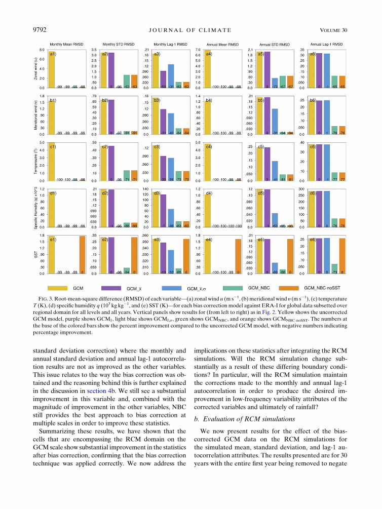
standard deviation correction) where the monthly and

annual standard deviation and annual lag-1 autocorrela-

tion results are not as improved as the other variables.

This issue relates to the way the bias correction was ob-

tained and the reasoning behind this is further explained

in the discussion in section 4b. We still see a substantial

improvement in this variable and, combined with the

magnitude of improvement in the other variables, NBC

still provides the best approach to bias correction at

multiple scales in order to improve these statistics.

Summarizing these results, we have shown that the

cells that are encompassing the RCM domain on the

GCMscale show substantial improvement in the statistics

after bias correction, confirming that the bias correction

technique was applied correctly. We now address the

implications on these statistics after integrating the RCM

simulations. Will the RCM simulation change sub-

stantially as a result of these differing boundary condi-

tions? In particular, will the RCM simulation maintain

the corrections made to the monthly and annual lag-1

autocorrelation in order to produce the desired im-

provement in low-frequency variability attributes of the

corrected variables and ultimately of rainfall?

b. Evaluation of RCM simulations

We now present results for the effect of the bias-

corrected GCM data on the RCM simulations for

the simulated mean, standard deviation, and lag-1 au-

tocorrelation attributes. The results presented are for 30

years with the entire first year being removed to negate

FIG. 3. Root-mean-square difference (RMSD) of each variable—(a) zonal wind u (m s21, (b)meridional wind y (m s21), (c) temperature

T (K), (d) specific humidity q (103 kg kg21, and (e) SST (K)—for each bias correction model against ERA-I for global data subsetted over

regional domain for all levels and all years. Vertical panels show results for (from left to right) as in Fig. 2. Yellow shows the uncorrected

GCM model, purple shows GCMx, light blue shows GCMx,s , green shows GCMNBC, and orange shows GCMNBC-noSST. The numbers at

the base of the colored bars show the percent improvement compared to the uncorrected GCMmodel, with negative numbers indicating

percentage improvement.

9792 JOURNAL OF CL IMATE VOLUME 30

the influence of model spinup. Here we present the

same figures as above showing the scatter of specific

humidity to identify qualitative improvement (with

results for all variables available in appendix B), fol-

lowed by a comparison of RMSDs for all variables.

The main differences in these and the following re-

sults are that they pertain to the regional climate

model and not a subset of the global data used above.

As such the resolutions of the following results are

those identified in the WRF Model configuration. In

the following results the CSIRO-driven WRF, and

corrected cases, are compared with the ERA-I-driven

WRF simulation to assess improvements in the bias

correction cases against the ‘‘ideal’’ WRF simulation

driven by ERA-I. It should be noted that the results of

the RCM simulated outputs are expected to be worse

than the corrections on the global scale shown above

as the RCM output was not directly bias corrected

while the GCM output was.

Figure 4 shows the scatterplot for specific humidity q

after running the RCM for each bias correction case. The

comparison dataset is that of the ERA-I-drivenWRF.We

see that when the RCM(GCM) was run throughWRF we

roughly see a similar scatter to the global data but at a

higher resolution (i.e., more data points). However, it does

appear that there is a noticeable improvement of the

monthly and annual mean values compared to the GCM.

This gives an indication that theWRFModel is creating an

‘‘improvement’’ over the GCM through the sole mecha-

nism of being run. Forcing the model with differing

boundaries produces similar integrated output. For the

other statistics there is a very similar spread of the values

before and after running WRF.

When we run WRF on the mean correction case we

see an improvement in the monthly mean, although it is

not improved as much as what we gained directly in the

GCM corrected results. There remains a spread around

the 458 line although it is slightly reduced compared to

the uncorrected simulation. The monthly and annual

standard deviations are also improved slightly with no

observable change in scatterplots for the other statistics.

This tendency of slight improvement in the monthly and

annual mean, and monthly and annual standard de-

viation, seems to remain relatively constant in the scat-

terplot results for specific humidity for the rest of the

bias correction cases. It is apparent that the statistics

FIG. 4. As in Fig. 2, but for the regional climate simulation output.

15 DECEMBER 2017 ROCHETA ET AL . 9793

here are not nearly as good as the statistics that we ob-

tained through the bias correction of the rawGCMfields

and that there are other processes occurring within the

RCM that are reducing the impact of the improvements

provided in the lateral and lower boundaries. This is

particularly important in the monthly and annual lag-1

autocorrelations, which do not showmuch improvement

in these scatterplots. This lack of improved RCM sim-

ulation skill will have deleterious consequences whenwe

look at low-frequency variability attributes that are re-

lated to these statistics. Additionally, the monthly mean

and standard deviation correction fails to improve the

monthly standard deviation of specific humidity no-

ticeably; however, there is some improvement in other

variables.

In a similar way to the global data, we now address the

RMSD values for all variables after theWRF simulation

run, which allows for a quantification of changes in sta-

tistics and an overview of how successful the RCM

simulation was in obtaining fields derived from the

forcing lateral and lower boundaries.

We see from Fig. 5 that themean correction reduces the

mean RMSD substantially, resulting in the order of 44%–

80% improvement, substantially less than the corrections

obtained directly on the GCM fields, which were ;99%

improvement. The improvement in annual mean, which

was;100% in theGCMdata, falls into the range of 68%–

80%. Modifying the mean now also has implications for

other statistics that did not occurwith theGCMcorrection.

For example, the annual standard deviation and annual

lag-1 autocorrelation of zonal wind u worsened by 7%

compared to the base case RCM(GCM) simulations

RMSD. There is also substantial improvement in the

monthly lag-1 autocorrelation even though these statistics

were not modified in the input conditions. This suggests

that WRF’s internal dynamics are propagating modifica-

tions of the LBCs into the domain in complex ways. This is

further exemplified by the consistent annual lag-1 RMSDs

FIG. 5. As in Fig. 3, but for regional climate simulation output. RMSDs are calculated using RCM(ERA-I) as the reference.

9794 JOURNAL OF CL IMATE VOLUME 30

in atmospheric variables being roughly equivalent to

the uncorrected RCM(GCM) simulation with the only

substantial improvements after RCM(GCMNBC) to

be found in the atmospheric and sea surface temper-

ature fields (T and SST). The remaining annual

RCM(GCMNBC) fields were equally erroneous as the

uncorrected simulation indicates that the corrections

in the input conditions were overridden by internal

model dynamics.

There are also several interesting findings related to

theRCM(GCMNBC-noSST) case. The SST fieldmaintains

its correction, in line with the magnitude of correction

obtained on the RCM(GCM) results, greater than the

atmospheric variables (280% for SST vs275% for T in

monthly mean RMSD, for example) as this field is not

passed through a relaxation zone like the atmospheric

fields. The SST field is forced on the surface layer every

five time steps regardless of the SST field in the prior

time step.

c. Effect of bias correction on Australian rainfall

We have seen above that through bias correcting the

atmospheric conditions that define the LBCs, we can

force some improvement in particular statistics of the

atmospheric variables in the RCM. But how does the

rainfall simulation change as a result of changes in

the atmospheric conditions? In this section we compare

the RCM simulation output to the ERA-I-driven WRF

andAWAPobservational rainfall datasets. Figure 6 shows

the RMSDs in rainfall over land for each bias correc-

tion technique against RCM(ERA-I) for the selected

temporal statistics. This figure identifies improve-

ments related toRCM(GCMx) on the order of from239%

to236% formonthly and annual mean RMSDs, which

are further improved slightly for the more advanced

correction cases. RCM(GCMx,s) produced changes

in the mean and standard deviation statistics roughly as

expected (i.e., with an improvement over the more basic

correction case). RCM(GCMNBC) also garnered similar

improvements to RCM(GCMx,s) in these more basic

statistics.

Although improvement from bias correction can be

gained in the first and second statistical moments, these

results are similar to Fig. 5 in that annual lag-1 auto-

correlation RMSD values are virtually unchanged for

any correction case compared to the uncorrected

RCM(GCM) simulation; in fact, the results presented

here show 20%–30% degradations. This raises two

possibilities: either the lack of correction on this statistic

is related to the reduction in the same statistic for the

atmospheric variables, or rainfall generation within

WRF is more dependent on other WRF conditions that

were not subject to the correction procedure for annual

lag-1 autocorrelations.

It is also clear from this figure that SSTs are an important

variable in corrections (in conjunction with corresponding

atmospheric variables) as the RCM(GCMNBC-noSST)

case produces the largest rainfall RMSDs over all

temporal scales and statistical measures, except for

annual lag-1 autocorrelations. In other words sim-

ply correcting the atmosphere without the SST field

not only reduces the ability of the RCM to produce

FIG. 6. Bar plot of RMSD using ERA-I-driven WRF as reference for each model in RCM for rainfall (mm) over the Australian

landmass for the statistics as in Fig. 2. Here yellow represents the uncorrectedGCM, purple showsGCMx, light blue showsGCMx,s, green

shows GCMNBC, and orange shows GCMNBC-noSST.

FIG. 7. As in Fig. 6, but using AWAP as the observational reference.

15 DECEMBER 2017 ROCHETA ET AL . 9795

FIG. 8. (a) Aggregated persistence scores using AWAP as the observational reference for 1–12-month

aggregations for (from top to bottom) RCM(ERA-I), RCM(GCM), RCM(GCMx), RCM(GCMx,s),RCM

(GCMNBC), and RCM(GCMNBC-noSST); (b),(c) as in (a), but for 12–24-month and 24–36-month aggregations,

respectively. Refer to section 2c for score descriptions.

9796 JOURNAL OF CL IMATE VOLUME 30

reasonable rainfall characteristics but also makes land-

based rainfall worse by up to a factor of 139%.

While the results from ERA-I-driven WRF represent

the target toward which we are correcting, it also con-

tains errors in the characteristics of interest. Figure 7

compares RMSDs of the modeled cases against AWAP

rainfall observations over the land and including an

additional bar which shows the RMSD of ERA-I-driven

WRF versus AWAP.

Here we see some limitations when bias correcting

toward ERA-I. In many ways, the ERA-I-driven WRF

simulation represents the ‘‘best case’’ expectation for

the result after bias correcting the LBCs toward ERA-I.

Thus, only in cases where the GCM-driven WRF per-

forms significantly worse than the ERA-I-driven WRF

can we reasonably expect bias correction of LBCs to

improve the model performance when compared to

observations. This is indeed the case for monthly

means where we see that bias correction of the LBCs

reduces the RMSD from the GCM-driven WRF

values toward the ERA-I-driven WRF values. For the

remaining statistics only small differences exist be-

tween the ERA-I-driven WRF and the GCM-driven

WRF, and hence LBC bias corrections would not be

expected to change these statistics substantially. It is

worth noting that despite this, both the monthly and

annual standard deviation are improved beyond the

ERA-I-driven WRF in the RCM(GCMx,s) and RCM

(GCMNBC) cases.

Combining Figs. 5 and 6 shows us that ERA-I-driven

WRF and GCM-driven WRF are different from each

other and bias correction of LBCs toward ERA-I can

make the simulations look more similar. Figure 7,

however, shows us that compared to observations when

averaged continentally, ERA-I-driven WRF and GCM-

drivenWRF have similar precipitation statistics and bias

correction of LBCs has relatively little impact. This

again suggests that the WRF Model physics and dy-

namics play a strong role in the production of pre-

cipitation within the domain.

d. Aggregated persistence score of precipitation

So far we have seen the effect of bias correction on

the global and regional scales in relation to modification

of the statistics that were corrected. Now we address

changes in the low-frequency variability of rainfall across

the Australian landmass using the APS, a persistence

metric, compared to AWAP observations, in a spatially

FIG. A1. As in Fig. 2, but for zonal wind u (m s21).

15 DECEMBER 2017 ROCHETA ET AL . 9797

explicit way. These results are presented for all models

and ERA-I-driven WRF over 1–12-month aggregations

(Fig. 8a), 12–24-month aggregations (Fig. 8b), and

24–36-month aggregations (Fig. 8c) to indicate the

ability of RCMs to correctly simulate observed persis-

tence attributes on intra- and interannual cycles.

The 1–12-month aggregations (Fig. 8a), or intra-annual

variability, show substantial improvement after mean

bias correction with additional improvement in RCM

(GCMx,s) compared to uncorrected RCM(GCM) model

output, which overestimates persistence attributes. The

gains from RCM(GCMNBC) are similar to those in RCM

(GCMx,s) where the additional lag-1 correction has a mi-

nor impact the 1–12-month APS. The APS values reduce

from a maximum in the raw RCM(GCM) of 16 over-

estimation of persistence on average to values much closer

to zero for the RCM(GCMx,s) and RCM(GCMNBC) ca-

ses. This shows that the intra-year variability can be suc-

cessfully corrected by modifying LBCs of the RCM to

produce improved precipitation persistence within the

model, but that most of this improvement is gained from a

mean and standard deviation correction.

Similar results are shown in both interannual vari-

ability cases of Figs. 8b and 8c, where RCM(GCMx,s)

leads to substantial improvement and the influence of

NBC is only marginal. This confirms the results pre-

sented in Fig. 7, which shows that annual lag-1 auto-

correlation RMSDs are almost identical between RCM

(GCMx,s) and RCM(GCMNBC). However, when we

look at Figs. 8a1–c1, we see the bias between RCM

(ERA-I) output and AWAP observation, which again

show the ‘‘best case’’ of correction we could have ex-

pected. We see in these figures that there is a sub-

stantial bias in the RCM(ERA-I)-generated rainfall

compared to AWAP although this bias is less than

from the raw RCM(GCM) simulation (Figs. 8a2–c2).

What is interesting is that RCM(GCMx,s) and

RCM(GCMNBC) actually improved the low-frequency

variability attributes more than this best case at least

for the 1–12- and 12–24-month aggregation cases.

What process led to this improvement is unknown but

clearly the effect of low-frequency variability in simu-

lated rainfall is not only driven by the lag-1 autocorrela-

tions in the atmosphere.

Finally, the effect of SST seen through comparing Figs.

8a5 with 8a6, 8b5 with 8b6, and 8c5 with 8c6 suggests that

the SSTs have a substantial influence on rainfall persis-

tence over much of Australia including the eastern

FIG. A2. As in Fig. 2, but for meridional wind y (m s21).

9798 JOURNAL OF CL IMATE VOLUME 30

seaboard and the southern edge across to southwestern

Australia, and a swath from northern Australia across to

the northeast.

4. Discussion

The results presented here have shown that correc-

tion of GCM data used to define boundary conditions

that force an RCM can improve the statistics that were

corrected, although the effect of the improvement on

the RCM is reduced compared to the GCM. Of in-

terest, especially for improving theWRFModel, is that

correcting for mean fields produces the largest im-

provement overall, but also the largest improvement in

rainfall low-frequency variability measured by the APS

in the regional simulation. The effectiveness of in-

creasingly complex techniques only adds small im-

provements to the rainfall characteristics. This means

that the act of correcting atmospheric variable lag-1

autocorrelation conditions does not lead to the ex-

pected improvement in the rainfall annual lag-1 auto-

correlation. This is because WRF removes much of the

improvement in the atmospheric fields of this metric,

and because WRF simulates ERA-I rainfall with

similar bias in annual lag-1 autocorrelations when

compared to AWAP observations regardless of its

‘‘improved’’ atmospheric lag-1 structure in the RCM.

There must be other factors within the WRF Model

that dictate the low-frequency variability attributes in

rainfall that are not related to the atmospheric low-

frequency variability attributes. Improving the low-

frequency variability structure of simulated rainfall

output should be further investigated to improve sim-

ulation and aid the use of this model in assessing hy-

drological climate change impact assessment.

a. Comparison with earlier approaches

We now compare our results with earlier studies to

identify commonalities between the ability of bias cor-

rection to improve RCM simulations. The results pre-

sented focus on WRF simulations, and in particular

those that compare the effectiveness of different bias

correction techniques on the simulation outcome. The

following papers used similar experimental design and

can be compared with the results discussed above:

d Xu and Yang (2012) performed a mean and standard

deviation bias correction on atmospheric variables

FIG. A3. As in Fig. 2, but for temperature T (K).

15 DECEMBER 2017 ROCHETA ET AL . 9799

and showed clear improvement in the simulation of

most variables assessed. Variance correction im-

provements were generally similar to mean correc-

tion for 2-m air temperature and precipitation with

some advantage from variance correction found

when assessing the whole 2-m air temperature

distribution.d Colette et al. (2012) performed a cumulative distri-

bution function transform (CDF-t) on atmospheric vari-

ables and found a reduction in the mean bias of several

downscaled variables. Of note was the lower overesti-

mation of precipitation in the RCM, but there were still

biases associated with low and high rainfall. As this

technique does not modify temporal variability, temper-

ature seasonality biases were found.d Bruyère et al. (2014) performed a number of bias

correction cases with the aim of improving hurricane

tracking in the Gulf of Mexico. The corrections were

limited to the climatological mean on differing sets of

input variables. The results showed that a mean

correction of all variables was best able to improve

the desired hurricane results.d White and Toumi (2013) found that linear mean bias

correction was more reliable and accurate compared

to nonlinear quantile–quantile bias correction of

RCM input due to the effect of spurious spatial vari-

ability in the QQ approaches as well as dynamical

inconsistencies in the relaxation zone.

The work presented in these papers identifies limita-

tions on bias correction similar to those that we found.

Namely, that mean correction improved the model

bias, yet correction of higher-order statistics generally

had a lesser effect, possibly dampened by internal

model dynamics, parameterizations, or through some

other means. This is most apparent in the case of monthly

standard deviation and annual lag-1 autocorrelations in

most atmospheric variables, although improvements are

clearer with SST corrections and, to a lesser extent, the

specific humidity and temperature fields.

b. Limitations of current study

Our experimental setup has several limitations that

may influence the results and the ability to draw addi-

tional conclusions from this work. Limitations of this

study can be broken into two groups: those that pertain

to the RCM model adopted, and those that arise from

the bias correction approaches used.

FIG. A4. As in Fig. 2, but for SST (K).

9800 JOURNAL OF CL IMATE VOLUME 30

The WRF Model is complex and contains alterna-

tive configurations of parameterizations, options, and

setup. We have chosen those that have been shown to

be appropriate over the domain but alternative setups

would influence the results. One major factor within

WRF that created the results shown is the configu-

ration of the relaxation zone, which uses a weighting

function to balance the atmospheric state in the outer

specified cells with those in the model domain. This

weighting does not account for atmospheric dynamics

and creates physical inconsistencies in these cells.

This combined with bias correction approaches that

do not attempt to maintain intervariable correlations

could lead to the results presented here. An addi-

tional limitation of the WRF configuration chosen is

that the Dudhia shortwave radiation scheme does not

resolve the ozone layer that would normally be con-

tained in a model extending to 0.5 hPa. However, as

the results presented pertain to the comparison of

different input data, which all use the same model

configuration, these results remain valid even though

the configuration negated the influence of a modeled

ozone layer.

This work has only focused on one RCM, driven by

one GCM. Couplings with different GCMs or using

other RCMs may lead to different results than those

presented here. Additionally, the focus of this work on

correcting rainfall attributes ignores potential im-

provement in other surface or atmospheric variables of

interest in other applications.

Limitations of the NBC approach relate primarily to

complexity and underlying assumptions within the

transfer model. Some examples are that NBC assumes

both datasets represent an autoregressive model of order

1 (AR1) across multiple time scales, and that the mag-

nitude of corrected values was limited by bounds that

were selected based on a sensitivity assessment to en-

sure that statistical corrections did not result in physi-

cally unrealistic values. This lead to a minor number of

poorly performing cells in the corrected statistics as

shown, for example, in the zonal wind u scatterplot in

appendix A. The primary limitation is that NBC does

not have a physical foundation for improving extreme

variable values, instead only correcting low-frequency

variability. As such, extreme events driven by finer

spatial scales than the monthly and annual corrections

FIG. B1. As in Fig. 4, but for zonal wind u (m s21).

15 DECEMBER 2017 ROCHETA ET AL . 9801

would not be improved through this technique. The

added drawback of performing corrections indepen-

dently across all LBC and lower boundary variables

may further complicate the representation of extreme

causing conditions.

c. Implications and future work

The implications of this work are quite substantial as it

clearly identifies that correction of LBCs and lower

boundaries do impact the resulting simulations, and it

illustrates that correction of persistence attributes at

monthly and yearly scales in the boundaries does not

translate effectively into simulations of atmospheric

variables or rainfall. This, in turn, raises several added

questions that need to be addressed in future research,

as follows:

1) How do sustained anomalies (such as those result-

ing from ENSO) in the LBCs manifest as rainfall

within RCMs? There is evidence showing that RCM

simulations do simulate ENSO anomalies consistently

with those simulated in GCM fields. But because our

results indicate that the better representation of in-

terannual persistence in the LBCs does not translate

as effectively to the finescale rainfall fields, the

question of how representation of sustained ENSO

anomalies in the boundaries translate to similar

representation in the rainfall needs to be investigated.

2) What is the relative importance of the various factors

that contribute to the outcomes presented here,

namely, the WRF parameterization and configura-

tions used, the domain size, the relaxation zone

considered for the LBCs, and the lower SST bound-

ary that is not modified by a relaxation zone in the

resulting simulation? Leading on from this is the

added question, what alterations are needed in these

settings for better simulation of low-frequency var-

iability in downscaled rainfall fields?

3) How can the bias correction procedure being adop-

ted be improved to better represent low-frequency

variability in resulting simulations? As discussed

before, the bias correction alternatives, though effec-

tive, still leave a lot to be desired. In the first instance,

biases in the joint relationship of the forcing vari-

ables are ignored (Mehrotra and Sharma 2015).

Second, each cell in the LBC or lower boundary

field is corrected independently of surrounding

cells. Third, the correction assumes that only two

FIG. B2. As in Fig. 4, but for meridional wind y (m s21).

9802 JOURNAL OF CL IMATE VOLUME 30

aggregation periods (monthly and annual) are im-

portant for all variables, which is a simplification

of the way low-frequency variability is manifested

in the climate system (Nguyen et al. 2016). Fourthly,

the choice of reanalysis dataset used to deter-

mine bias correction factors and the ability of the

reanalysis product to adequately capture regional

statistics of interest play a role in resultant skill of

the corrected simulation (Moalafhi et al. 2016).

Finally, implications of the assumption of bias

stationarity must be addressed (Nahar et al. 2017)

if we attempt to apply these correction approaches

to future simulations.

5. Conclusions

Low-frequency variability in rainfall is an impor-

tant characteristic for water resources management

and GCMs are known to poorly simulate this vari-

ability in rainfall. This work attempted to apply a bias

correction technique to improve low-frequency var-

iability in RCM input boundary conditions and

compared the results against simpler boundary bias

corrections.

This work shows that simple bias correction—

particularly that of the distributions mean—can be very

effective in reducing bias in the RCM simulation, thereby

improving output for impact model use. However, we

also show that the effectiveness of improved annual lag-1

autocorrelation characteristics in the RCM boundaries

does not translate as well into the RCM simulation of

atmospheric variables or rainfall.

Low-frequency variability can be imparted into

modeled rainfall, but interestingly the major im-

provement comes from mean correction with standard

deviation and finally lag-1 autocorrelations corrections

only adding minimally to the mean correction. Al-

though atmospheric variable annual lag-1 corrections

were reduced in the atmosphere after NBC, either

through processes in the LBCs or through inter-

nal model dynamics, it is clear that the atmospheric

variables’ low-frequency variability does not play the

dominant role in driving rainfall low-frequency vari-

ability. This is shown through the differences in low-

frequency variability in atmospheric variables between

GCM-driven and ERA-I-driven WRF producing sim-

ilar rainfall APS compared to AWAP. In this study

improvements in the atmospheric low-frequency

FIG. B3. As in Fig. 4, but for temperature T (K).

15 DECEMBER 2017 ROCHETA ET AL . 9803

variability did not translate directly into improvements

in rainfall low-frequency variability and further in-

vestigation is needed to identify theWRF processes that

control this rainfall characteristic.

Acknowledgments. Thanks go to Rajeshwar Mehrotra

for his assistance in bias correction. The authors thank the

anonymous reviewers for their valuable comments and

suggestions which improved the quality of the paper.

Funding for this research came from the Australian

Research Council (FT110100576 and FT100100197)

and the Peter Cullen Postgraduate Scholarship. This

research was undertaken with the assistance of re-

sources provided at the NCI National Facility systems

at the Australian National University through the

National Computational Merit Allocation Scheme

supported by the Australian Government. We ac-

knowledge the modeling groups for making their

model output available for analysis, the PCMDI for

collecting and archiving, and the WGCM for organiz-

ing this data. ERA-I data were obtained from the

European Centre for Medium-Range Weather Fore-

casts (ECMWF) online archive catalogue. We thank the

Australian Water Availability Project (AWAP) Team,

and CSIROMarine andAtmosphericResearch (CMAR)

for making available the AWAP rainfall dataset.

APPENDIX A

Scatterplots of Global Variables over theAustralasian CORDEX Domain

Scatterplots for the other— u, y, T, and SST—corrected

variables as in Fig. 2 (Figs. A1–A4).

APPENDIX B

Scatterplots of Regional Simulation Output

Scatterplots for the other—u, y, T, and SST—corrected

variables as in Fig. 4 (Figs. B1–B4).

REFERENCES

Brands, S., S. Herrera, J. Fernández, and J. M. Gutiérrez, 2013:How well do CMIP5 Earth system models simulate present

climate conditions in Europe and Africa? A performance

FIG. B4. As in Fig. 4, but for SST (K).

9804 JOURNAL OF CL IMATE VOLUME 30

comparison for the downscaling community.Climate Dyn., 41,

803–817, doi:10.1007/s00382-013-1742-8.

Bruyère, C. L., J. M. Done, G. J. Holland, and S. Fredrick, 2014:

Bias corrections of global models for regional climate simu-

lations of high-impact weather. Climate Dyn., 43, 1847–1856,

doi:10.1007/s00382-013-2011-6.

Caldwell, P.,H.-N. S.Chin,D.C.Bader, andG.Bala, 2009:Evaluation

of a WRF dynamical downscaling simulation over California.

Climatic Change, 95, 499–521, doi:10.1007/s10584-009-9583-5.

Capps, S. B., and C. S. Zender, 2008: Observed and CAM3 GCM

sea surface wind speed distributions: Characterization, com-

parison, and bias reduction. J. Climate, 21, 6569–6585,

doi:10.1175/2008JCLI2374.1.

Casanueva, A., and Coauthors, 2016: Daily precipitation statistics

in a EURO-CORDEX RCM ensemble: Added value of raw

and bias-corrected high-resolution simulations. Climate Dyn.,

47, 719–737, https://doi.org/10.1007/s00382-015-2865-x.

Colette, A., R. Vautard, and M. Vrac, 2012: Regional climate

downscaling with prior statistical correction of the global cli-

mate forcing. Geophys. Res. Lett., 39, L13707, doi:10.1029/

2012GL052258.

Dee, D. P., and Coauthors, 2011: The ERA-Interim reanalysis:

Configuration and performance of the data assimilation system.

Quart. J. Roy. Meteor. Soc., 137, 553–597, doi:10.1002/qj.828.

Dudhia, J., 1989: Numerical study of convection observed during

the Winter Monsoon Experiment using a mesoscale two-

dimensional model. J. Atmos. Sci., 46, 3077–3107, doi:10.1175/

1520-0469(1989)046,3077:NSOCOD.2.0.CO;2.

Ehret, U., E. Zehe, V.Wulfmeyer, K.Warrach-Sagi, and J. Liebert,

2012: HESS opinions: ‘‘Should we apply bias correction to

global and regional climate model data?’’ Hydrol. Earth Syst.

Sci., 16, 3391–3404, doi:10.5194/hess-16-3391-2012.

Evans, J. P., and M. F. McCabe, 2013: Effect of model resolution

on a regional climate model simulation over southeast Aus-

tralia. Climate Res., 56, 131–145, doi:10.3354/cr01151.

——,M. Ekström, and F. Ji, 2012: Evaluating the performance of a

WRF physics ensemble over South-East Australia. Climate

Dyn., 39, 1241–1258, doi:10.1007/s00382-011-1244-5.

Hempel, S., K. Frieler, L. Warszawski, J. Schewe, and F. Piontek,

2013: A trend-preserving bias correction—The ISI-MIP ap-

proach. Earth Syst. Dyn., 4, 219–236, doi:10.5194/

esdd-4-49-2013.

Holland, G., J. Done, C. Bruyere, C. K. Cooper, and A. Suzuki,

2010: Model investigations of the effects of climate variability

and change on future Gulf of Mexico tropical cyclone activity.

Offshore Technology Conf. 2010, Houston, TX, OTC,

doi:10.4043/20690-MS.

Janjic, Z. I., 1994: The step-mountain eta coordinate model: Fur-

ther developments of the convection, viscous sublayer, and

turbulence closure schemes. Mon. Wea. Rev., 122, 927–945,

doi:10.1175/1520-0493(1994)122,0927:TSMECM.2.0.CO;2.

John, V. O., and B. J. Soden, 2007: Temperature and humidity

biases in global climate models and their impact on climate

feedbacks. Geophys. Res. Lett., 34, L18704, doi:10.1029/

2007GL030429.

Johnson, F., and A. Sharma, 2011: Accounting for interannual

variability: A comparison of options for water resources cli-

mate change impact assessments. Water Resour. Res., 47,

W04508, doi:10.1029/2010WR009272.

——, and ——, 2012: A nesting model for bias correction of vari-

ability at multiple time scales in general circulation model

precipitation simulations. Water Resour. Res., 48, W01504,

doi:10.1029/2011WR010464.

——, S. Westra, A. Sharma, and A. J. Pitman, 2011: An assessment

of GCM skill in simulating persistence across multiple time

scales. J. Climate, 24, 3609–3623, doi:10.1175/2011JCLI3732.1.Jones, D. A., W. Wang, and R. Fawcett, 2009: High-quality spatial

climate data-sets for Australia. Aust. Meteor. Mag., 58, 233–

248, www.bom.gov.au/amm/docs/2009/jones.pdf.

Jury, M. W., A. F. Prein, H. Truhetz, and A. Gobiet, 2015: Eval-

uation of CMIP5 models in the context of dynamical down-

scaling over Europe. J. Climate, 28, 5575–5582, doi:10.1175/

JCLI-D-14-00430.1.

Kim, K. B., H.-H. Kwon, andD. Han, 2015: Bias correctionmethods

for regional climate model simulations considering the distri-

butional parametric uncertainty underlying the observations.

J. Hydrol., 530, 568–579, doi:10.1016/j.jhydrol.2015.10.015.——, ——, and ——, 2016: Precipitation ensembles conforming to

natural variations derived from a regional climate model

using a new bias correction scheme. Hydrol. Earth Syst. Sci.,

20, 2019–2034, doi:10.5194/hess-20-2019-2016.

Lim, K.-S. S., and S.-Y. Hong, 2010: Development of an effective

double-moment cloud microphysics scheme with prognos-

tic cloud condensation nuclei (CCN) for weather and

climate models.Mon. Wea. Rev., 138, 1587–1612, doi:10.1175/

2009MWR2968.1.

Meehl, G. A., C. Covey, K. E. Taylor, T. Delworth, R. J. Stouffer,

M. Latif, B. McAvaney, and J. F. B. Mitchell, 2007: The

WCRP CMIP3 multimodel dataset: A new era in climate

change research. Bull. Amer. Meteor. Soc., 88, 1383–1394,

doi:10.1175/BAMS-88-9-1383.

Mehrotra, R., and A. Sharma, 2012: An improved standardization

procedure to remove systematic low frequency variability

biases in GCM simulations. Water Resour. Res., 48, W12601,

doi:10.1029/2012WR012446.

——, and ——, 2015: Correcting for systematic biases in multiple

raw GCM variables across a range of timescales. J. Hydrol.,

520, 214–223, doi:10.1016/j.jhydrol.2014.11.037.

Meyer, J. D. D., and J. Jin, 2016: Bias correction of the CCSM4

for improved regional climate modeling of the North Ameri-

can monsoon. Climate Dyn., 46, 2961–2976, doi:10.1007/

s00382-015-2744-5.

Mlawer, E. J., S. J. Taubman, P. D. Brown, M. J. Iacono, and S. A.

Clough, 1997: Radiative transfer for inhomogeneous atmo-

spheres: RRTM, a validated correlated-k model for the

longwave. J. Geophys. Res., 102, 16 663–16 682, doi:10.1029/

97JD00237.

Moalafhi, D. B., J. P. Evans, and A. Sharma, 2016: Evaluating

global reanalysis datasets for provision of boundary conditions

in regional climate modelling. Climate Dyn., 47, 2727–2745,

https://doi.org/10.1007/s00382-016-2994-x.

Nahar, J., F. Johnson, andA. Sharma, 2017: Assessing the extent of

non-stationary biases in GCMs. J. Hydrol., 549, 148–162,

doi:10.1016/j.jhydrol.2017.03.045.

Nguyen, H., R. Mehrotra, and A. Sharma, 2016: Correcting

for systematic biases inGCMsimulations in the frequency domain.

J. Hydrol., 538, 117–126, doi:10.1016/j.jhydrol.2016.04.018.

Olson, R., J. P. Evans, A. Di Luca, and D. Argueso, 2016: The

NARCliM Project: Model agreement and significance of cli-

mate projections. Climate Res., 69, 209–227, https://doi.org/

10.3354/cr01403.

Ratnam, J. V., S. K. Behera, T. Doi, S. B. Ratna, and

W. A. Landman, 2016: Improvements to theWRF seasonal hind-

casts over South Africa by bias correcting the driving SINTEX-

F2v CGCM fields. J. Climate, 29, 2815–2829, doi:10.1175/

JCLI-D-15-0435.1.

15 DECEMBER 2017 ROCHETA ET AL . 9805

Rocheta, E., M. Sugiyanto, F. Johnson, J. Evans, and A. Sharma,

2014a: How well do general circulation models represent low-

frequency rainfall variability? Water Resour. Res., 50, 2108–

2123, doi:10.1002/2012WR013085.

——, J. P. Evans, and A. Sharma, 2014b: Assessing atmospheric

bias correction for dynamical consistency using potential

vorticity.Environ. Res. Lett., 9, 124010, doi:10.1088/1748-9326/

9/12/124010.

Rojas, M., and A. Seth, 2003: Simulation and sensitivity in a

nested modeling system for South America. Part II: GCM

boundary forcing. J. Climate, 16, 2454–2471, doi:10.1175/

1520-0442(2003)016,2454:SASIAN.2.0.CO;2.

Ruiz-Ramos, M., A. Rodríguez, A. Dosio, C. M. Goodess,

C. Harpham, M. I. Mínguez, and E. Sánchez, 2016: Compar-

ing correction methods of RCM outputs for improving

crop impact projections in the Iberian Peninsula for 21st

century. Climatic Change, 134, 283–297, doi:10.1007/

s10584-015-1518-8.

Skamarock, W. C., and Coauthors, 2008: A description of the

Advanced Research WRF version 3. NCAR Tech. Note

NCAR/TN-4751STR, 113 pp., doi:10.5065/D68S4MVH.

Teutschbein, C., and J. Seibert, 2012: Bias correction of regional

climate model simulations for hydrological climate-change

impact studies: Review and evaluation of different methods.

J. Hydrol., 456–457, 12–29, doi:10.1016/j.jhydrol.2012.05.052.

Tewari, M., and Coauthors, 2004: Implementation and verification

of the unified Noah land surface model in the WRF model.

20th Conf. on Weather Analysis and Forecasting/16th Conf. on

Numerical Weather Prediction, Seattle, WA, Amer. Meteor.

Soc., 14.2a, https://ams.confex.com/ams/84Annual/techprogram/

paper_69061.htm.

van Ulden, A., and G. van Oldenborgh, 2006: Large-scale at-

mospheric circulation biases and changes in global climate

model simulations and their importance for climate change

in central Europe. Atmos. Chem. Phys., 6, 863–881,

doi:10.5194/acp-6-863-2006.

Vial, J., and J. Osborn, 2012: Assessment of atmosphere–ocean

general circulation model simulations of winter Northern

Hemisphere atmospheric blocking. Climate Dyn., 39, 95–112,

https://doi.org/10.1007/s00382-011-1177-z.

Vrac, M., and P. Friederichs, 2015: Multivariate—intervariable,

spatial, and temporal—bias correction. J. Climate, 28, 218–

237, doi:10.1175/JCLI-D-14-00059.1.

Warner, T. T., R. A. Peterson, and R. E. Treadon, 1997: A tuto-

rial on lateral boundary conditions as a basic and potentially

serious limitation to regional numerical weather prediction.

Bull. Amer. Meteor. Soc., 78, 2599–2617, doi:10.1175/

1520-0477(1997)078,2599:ATOLBC.2.0.CO;2.

White, R. H., and R. Toumi, 2013: The limitations of bias cor-

recting regional climate model inputs.Geophys. Res. Lett., 40,

2907–2912, doi:10.1002/grl.50612.

Wu,W., A. H. Lynch, andA. Rivers, 2005: Estimating the uncertainty

in a regional climatemodel related to initial and lateral boundary

conditions. J. Climate, 18, 917–933, doi:10.1175/JCLI-3293.1.

Xu, Z., and Z.-L. Yang, 2012: An improved dynamical downscaling

method with GCM bias corrections and its validation with 30

years of climate simulations. J. Climate, 25, 6271–6286, https://

doi.org/10.1175/JCLI-D-12-00005.1.

9806 JOURNAL OF CL IMATE VOLUME 30