ORIGINAL PAPER

Evaluating rainfall patterns using physics scheme ensemblesfrom a regional atmospheric model

Fei Ji & Marie Ekström & Jason P. Evans & Jin Teng

Received: 28 November 2012 /Accepted: 8 April 2013# Springer-Verlag Wien 2013

Abstract This study evaluated the ability of WeatherResearch and Forecasting (WRF) multi-physics ensemblesto simulate storm systems known as East Coast Lows(ECLs). ECLs are intense low-pressure systems that developoff the eastern coast of Australia. These systems can causesignificant damage to the region. On the other hand, thesystems are also beneficial as they generate the majority ofhigh inflow to coastal reservoirs. It is the common interest ofboth hazard control and water management to correctlycapture the ECL features in modeling, in particular, toreproduce the observed spatial rainfall patterns. We simulat-ed eight ECL events using WRF with 36 model configura-tions, each comprising physics scheme combinations of twoplanetary boundary layer (pbl), two cumulus (cu), threemicrophysics (mp), and three radiation (ra) schemes. Theperformance of each physics scheme combination and theensembles of multiple physics scheme combinations wereevaluated separately. Results show that using the ensembleaverage gives higher skill than the median performer withinthe ensemble. More importantly, choosing a composite av-erage of the better performing pbl and cu schemes cansubstantially improve the representation of high rainfall bothspatially and quantitatively.

1 Introduction

East Coast Lows (ECLs) are intense low-pressure systemsthat occur off the eastern coast of Australia. Extreme rainfallevents associated with ECLs frequently cause significantflash flooding near the coast, as well as major flooding inriver systems with headwaters in the Great Dividing Range.In spite of its destructive capacity, the rainfall associatedwith ECLs has a beneficial role for coastal communities, asit provides significant inflow to coastal storages along theNew South Wales (NSW) coast (Pepler and Rakich 2010).Large events can even provide inflow to the headwaters ofwestern flowing rivers, particularly in northeastern NSW. Itis important for both hazard control and water managementto correctly capture the ECL features in modeling, in par-ticular, to reproduce the observed rainfall amounts and spa-tial patterns.

The Weather Research and Forecasting (WRF) model(Skamarock et al. 2008) is a numerical weather predictionand atmospheric simulation system designed for operationalforecasting, atmospheric research, and dynamical downscal-ing of Global Climate Models. Previous studies have shownthat the WRF model performs well for simulating the regionalclimate of south-eastern Australia (Evans and McCabe 2010,2013; Evans and Westra 2012). Evans et al. (2012) evaluatedphysics scheme combinations for hind-cast simulations offour ECL events using the WRF model. The authors investi-gated the influence of selecting different planetary boundarylayer (pbl), cumulus (cu), microphysics (mp), and radiation(ra) schemes on accuracy of maximum and minimum temper-ature, wind speed, mean sea level pressure, and rainfall.Similar sensitivity study was done for other regions too(Yuan et al. 2012; Jankov et al. 2005; Awan et al. 2011). Forexample, Yuan et al. (2012) used the WRF model configuredwith two alternative schemes of mp, cu, ra, and land surfacephysics schemes when forecasting winter precipitation in

F. Ji (*)NSW Office of Environment and Heritage, 11 Farrer Place,Queanbeyan, NSW 2620, Australiae-mail: fei.ji@environment.nsw.gov.au

M. Ekström : J. TengCSIRO Land and Water, GPO Box 1666, Canberra, ACT 2601,Australia

J. P. EvansClimate Change Research Centre, University of New South Wales,Anzac Pde, Sydney, NSW 2052, Australia

Theor Appl ClimatolDOI 10.1007/s00704-013-0904-2

China. The authors of these studies struggled to identifya single “best” physics scheme combination for all vari-ables, although it was clear that some combinationsperformed better than others for certain variables(Evans et al. 2012).

While sensitivity analysis cannot agree on a best modelconfiguration (Jankov et al. 2005; Evans et al. 2012), othermethods can be utilized to maximize the information gainedfrom multiple model runs using different parameterizations.Ensemble averaging is one of them, which is widely used inweather forecasting, seasonal predictions, and climate simu-lations (Fraedrich and Leslie 1987; Hagedorn et al. 2005;Phillips and Gleckler 2006; Schwartz et al. 2010; Schaller etal. 2011). Many studies have investigated the ensemble aver-ages of various regional climate models and perturbed initialconditions in simulating regional rainfall (Cocke and LaRow2000; Yuan and Liang 2011; Carril et al. 2012; Ishizaki et al.2012). Some of them showed that an ensemble average hadskill in reproducing heavy rainfall events (Yuan and Liang2011; Yuan et al. 2012), while others reported that the resultswere far from satisfactory (Carril et al. 2012).

In this paper, we evaluated the skill of ensemble averages(for the full ensemble and subsets of particular physicsschemes) relative to the use of individual ensemble membersto capture spatial and distributional properties of rainfall as-sociated with eight ECLs. We used the same physics schemecombinations as those used by Evans et al. (2012) but extend-ed the modeling to cover four more events, in order to give acomplete representation of the different types of synopticevents typically associated with ECLs (Speer et al. 2009).

2 Method

2.1 Physics scheme ensemble and model domain

This study used version 3.2.1 of WRF with the AdvancedResearch WRF dynamical core (Skamarock et al. 2008).Initial and boundary conditions were provided by European

Centre for Medium-Range Weather Forecasts interim re-analyses (ERA Interim) (Dee et al. 2011). The experimentalconfiguration consists of: 2 pbl, 2 cu, 3 ra, and 3 mp schemes,giving a total of 36 runs for each event (Table 1). The fulldetails of the experiment setup are described in Evans et al.(2012).

Two model domains with one-way nesting (with spectralnudging of wind and geopotential above 500 hpa in theouter domain) were used in this study (see Fig. 1), with gridspacing of 50 and 10 km for the outer and inner modeldomain, respectively. Both domains had 30 vertical levels.Each run was started 1 week prior to the event for a 2-weekperiod, thus encompassing pre- and post-storm days. Thetotal number of events simulated and resolution chosen werelimited by the available computational resources.

2.2 Case study periods

Using mean sea level pressure, wind speed, rainfall, andwave height, Speer et al. (2009) identified six different typesof ECLs: (1) ex-tropical cyclones, (2) inland trough lows,(3) easterly trough lows, (4) wave on front lows, (5)decaying front lows, and (6) lows in the westerlies. UnlikeEvans et al. (2012), our study of eight ECL events includesexamples of all common synoptic ECL types (Table 2). Theevents were subjectively named based on the location,timing, or type of event.

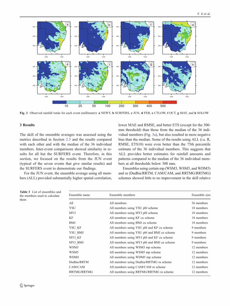
The eight ECL events were subjectively divided into twocategories (strong and weak) according to the observedrainfall amount. Four strong events (NEWY, SURFERS,JUN, and FEB) generally produced more than 200-mmcumulate rainfall and caused regional or local flooding. Incontrast, four weak events (CTLOW, OCT, MAY andSOLOW) generated less rainfall.

2.3 Observation and evaluation methodology

Gridded daily rainfall data over land with ∼5-km horizontalgrid spacing obtained from the Australian Water Availability

Table 1 WRF physics parameterization schemes used in the study

Physics schemes Options

Planetary boundary layer/surface layer Yonsei University (YSU)/Similaritytheory (MM5) (Hong et al. 2006;Paulson 1970; Webb 1970)

Mellor-Yamada-Janjic (MYJ)/Similaritytheory (Eta) (Janjic 1994)

Cumulus convection Kain-Fritsch (Kain and Fritsch 1990, 1993;Kain 2004)

Betts-Miller-Janjic (Betts and Miller 1986;Betts 1986; Janjic 1994, 2000)

Cloud microphysics WSM 3 class (Hong et al. 2004; Hongand Lim 2006; Dudhia 1989)

WSM 5 class (Hong et al. 2004;Hong and Lim 2006)

WDM 5 class

Radiation (long/short wave) RRTM/Dudhia (Mlawer et al. 1997;Dudhia 1989)

CAM/CAM(Collins et al. 2004)

RRTMG/RRTMG(Clough et al. 2005)

Land surface Noah LSM (Chen and Dudhia 2001)

F. Ji et al.

Project (AWAP) (Jones et al. 2009) were used for evaluationof model simulations. For the evaluation, 13-days accumu-lated AWAP rainfall was re-gridded to the 10-km resolutiondomain. Figure 2 shows accumulated AWAP rainfall mapsfor the eight ECL events.

The first day of each simulation was considered asthe spin-up period, and was hence excluded from theanalysis. The skill of each WRF physics scheme com-bination and their ensembles to simulate accumulatedrainfall was assessed using: spatial correlation (R), bias,mean absolute error (MAE), root mean square error(RMSE), and equitable threat score (ETS), also knownas the Gilbert Skill Score (Wilks 2006). Higher valuesof R and ETS indicate better forecasts, with a perfectETS achieving a score of 1. An ETS below zero in-dicates that random chance would provide a better sim-ulation than the model. MAE, RMSE and bias are allbetter as they approach zero.

The ETS is commonly used in forecast verification toinvestigate the overall spatial performance of the simula-tions for different rainfall thresholds (10, 25, 50, 100, 200,and 300 mm for all ECL events). It should be noted that the

higher rainfall thresholds have smaller sample sizes withthe 200-mm threshold sampling 1,136 grid points andthe 300-mm threshold sampling only 197 grid pointsfrom AWAP. For each threshold, an observation can beclassified as either: “a” (forecast and observed agree on ex-ceedance of threshold, i.e., hits), “d” (forecast and observedagree on non-exceedance of threshold), “c” (exceeded inobserved but not in forecast, i.e., missed event), and “b”(exceeded in forecast but not in observed, i.e. falsealarm). Having classified all grid cells according to a–d, theETS is then calculated as ETS ¼ a� arð Þ aþ bþ c� arð Þ= ,where ar is the number of hits due to random chance and isgiven by ar ¼ aþ bð Þ � aþ cð Þ aþ bþ cþ dð Þ= .

2.4 Ensemble integration

Ensemble averages were calculated for each event, using all36 members and subsets of runs simulated with common pbl,cu, mp, or ra physics schemes. The names and the collectionof runs used in ensembles are summarized in Table 3. Forexample, the “YSU” ensemble is averaged over the 18 runsthat use the YSU pbl scheme.

Fig. 1 Topographic mapshowing WRF model domainswith grid spacing of about 50and 10 km for the outer andinner domain, respectively(inner domain marked by redbox). All evaluations areconducted in the inner domainminus a border of six-grid cells

Table 2 Eight events used in thestudy Name Occurred on Type Intensity Impact

MAY 19 May 2007 Lows in westerlies Weak Widespread rain

NEWY 8 Jun 2007 Easterly trough low Strong Extensive flooding

JUN 14 Jun 2007 Decaying front low Strong Significant rain

OCT 31 Oct 2007 Inland trough low Weak Widespread rain

CTLOW 4 Nov 2007 lows in westerlies Weak Widespread rain

SURFERS 4 Jan 2008 Ex-tropical cyclone Strong Flash flooding

SOLOW 23 Aug 2008 Wave on a front low Weak Widespread showers

FEB 8 Feb 2009 Inland trough low Strong Significant widespread rain

Evaluating rainfall patterns using physics scheme ensembles

3 Results

The skill of the ensemble averages was assessed using themetrics described in Section 2.3 and the results comparedwith each other and with the median of the 36 individualmembers. Inter-event comparisons showed similarity in re-sults for all but the SURFERS event. Therefore, in thissection, we focused on the results from the JUN event(typical of the seven events that give similar results) andthe SURFERS event to demonstrate our findings.

For the JUN event, the ensemble average using all mem-bers (ALL) provided substantially higher spatial correlation,

lower MAE and RMSE, and better ETS (except for the 300-mm threshold) than those from the median of the 36 indi-vidual members (Fig. 3a), but also resulted in more negativebias than the median. Some of the results using ALL (i.e. R,RMSE, ETS10) were even better than the 75th percentileestimate of the 36 individual members. This suggests thatALL provides better estimates for rainfall amounts andpatterns compared to the median of the 36 individual mem-bers at all thresholds below 300 mm.

Ensembles using certain mp (WSM3,WSM5, andWDM5)and ra (Dudhia/RRTM, CAM/CAM, and RRTMG/RRTMG)schemes showed little to no improvement in the skill relative

Fig. 2 Observed rainfall totals for each event (millimeter): a NEWY, b SURFERS, c JUN, d FEB, e CTLOW, f OCT, g MAY, and h SOLOW

Table 3 List of ensembles andthe members used to calculatethem

Ensemble name Ensemble members Ensemble size

All All members 36 members

YSU All members using YSU pbl scheme 18 members

MYJ All members using MYJ pbl scheme 18 members

KF All members using KF cu scheme 18 members

BMJ All members using BMJ cu scheme 18 members

YSU_KF All members using YSU pbl and KF cu scheme 9 members

YSU_BMJ All members using YSU pbl and BMJ cu scheme 9 members

MYJ_KF All members using MYJ pbl and KF cu scheme 9 members

MYJ_BMJ All members using MYJ pbl and BMJ cu scheme 9 members

WSM3 All members using WSM3 mp scheme 12 members

WSM5 All members using WSM5 mp scheme 12 members

WDM5 All members using WDM5 mp scheme 12 members

Dudhia/RRTM All members using Dudhia/RRTMG ra scheme 12 members

CAM/CAM All members using CAM/CAM ra scheme 12 members

RRTMG/RRTMG All members using RRTMG/RRTMG ra scheme 12 members

F. Ji et al.

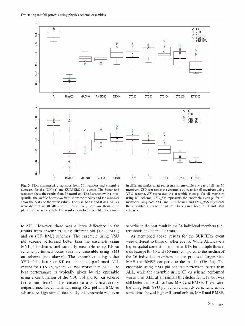
to ALL. However, there was a large difference in theresults from ensembles using different pbl (YSU, MYJ)and cu (KF, BMJ) schemes. The ensemble using YSUpbl scheme performed better than the ensemble usingMYJ pbl scheme, and similarly ensemble using KF cuscheme performed better than the ensemble using BMJcu scheme (not shown). The ensembles using eitherYSU pbl scheme or KF cu scheme outperformed ALLexcept for ETS 25, where KF was worse than ALL. Thebest performance is typically given by the ensembleusing a combination of the YSU pbl and KF cu scheme(nine members). This ensemble also considerablyoutperformed the combination using YSU pbl and BMJ cuscheme. At high rainfall thresholds, this ensemble was even

superior to the best result in the 36 individual members (i.e.,thresholds at 200 and 300 mm).

As mentioned above, results for the SURFERS eventwere different to those of other events. While ALL gave ahigher spatial correlation and better ETS for multiple thresh-olds (except for 10 and 300 mm) compared to the median ofthe 36 individual members, it also produced larger bias,MAE and RMSE compared to the median (Fig. 3b). Theensemble using YSU pbl scheme performed better thanALL, while the ensemble using KF cu scheme performedworse than ALL at all rainfall thresholds for ETS but wasstill better than ALL for bias, MAE and RMSE. The ensem-ble using both YSU pbl scheme and KF cu scheme at thesame time showed higher R, smaller bias, MAE and RMSE,

Fig. 3 Plots summarizing statistics from 36 members and ensembleaverages for the JUN (a) and SURFERS (b) events. The boxes andwhiskers show the results from 36 members. The boxes show the inter-quartile, the middle horizontal lines show the median and the whiskersshow the best and the worst values. The bias, MAE and RMSE valueswere divided by 30, 40, and 80, respectively, to allow them to beplotted in the same graph. The results from five ensembles are shown

in different markers. All represents an ensemble average of all the 36members, YSU represents the ensemble average for all members usingYSU scheme, KF represents the ensemble average for all membersusing KF scheme, YSU_KF represents the ensemble average for allmembers using both YSU and KF schemes, and YSU_BMJ representsthe ensemble average for all members using both YSU and BMJschemes

Evaluating rainfall patterns using physics scheme ensembles

and better skill at rainfall threshold below 100 mm com-pared to ALL, but the results were poorer at the 100- and200-mm rainfall thresholds.

4 Discussion

Ensemble averages have been found to perform consistentlyas well as, if not better than, the median of individualmembers when evaluated using common metrics in weatherforecasting, seasonal predictions and climate simulations(Fraedrich and Leslie 1987; Hagedorn et al. 2005; Phillipsand Gleckler 2006; Schwartz et al. 2010; Schaller et al.2011). For many of these metrics (e.g., bias, RMSE), en-semble averaging smoothens the field of interest, thus re-moving any large errors present in the individual ensemblemembers. However, this smoothing reduces the outliervalues and hence the ability to capture extremes. Resultspresented in Fig. 3 suggest that judicial choice of ensemblemembers allows the high rainfall centers to be captured byan ensemble average. For all events, assessments showedthat the ensemble mean for all members (ALL) and formembers using YSU pbl scheme (YSU) provided betterestimates for rainfall amounts and patterns compared to themedian of the individual members, even though they alsoresulted in larger bias, MAE and RMSE for the SURFERSevent relative to the median. The ensemble using the com-bination of the YSU pbl scheme and KF cu scheme(YSU_KF) was superior to all the other ensembles for seven

of the eight events. For SURFER event, the ensemble usingthe combination of the YSU pbl scheme and BMJ cuscheme (YSU_BMJ) gave the best performance for ETS100–300.

The unique response of SURFER prompted further in-vestigation into the synoptic conditions prevailing duringthis event. Comparing the complete rainfall field from WRF(i.e., including ocean grid cells) with observational rainfalldata, we propose that the geographical positioning of themain rainfall center of SURFER relative to the observationalrainfall data set could provide an explanation for the differ-ent behavior of SURFER relative to the other events. Asdescribed in Evans et al. (2012), the SURFERS event de-veloped from a tropical low that persisted for 5 to 6 daysover the Coral Sea, classified as an ex-Tropical Cyclone(xTC) type by Speer et al. (2009). While SURFER causedflash flooding throughout the region including SurfersParadise in Queensland, information from satellite imagesand Climate Prediction Center Merged Analysis ofPrecipitation showed that the major rainfall center was off-shore, and hence was not captured in the land-based AWAPobservations, whereas for all other events, the major rainfallcenters were on land. As the rainfall evaluation wasconducted only over land, the SURFER simulations wereassessed on conditions peripheral to the main storm center.Thus, we propose that geographical positioning of the mainrainfall center of SURFER relative to the observationalrainfall dataset could provide an explanation for the differ-ent behavior of SURFER relative to the other events.

-0.060-0.040-0.0200.0000.0200.0400.0600.080

Dif

fere

nce

rel

ativ

e to

AL

L

Metrics

for eight events

en_YSU

en_KF

en_YSU_KF

-0.060-0.040-0.0200.0000.0200.0400.0600.080

Dif

fere

nce

rel

ativ

e to

AL

L

Metrics

for seven events b

en_YSU

en_KF

en_YSU_KF

aFig. 4 Difference between thethree ensembles (YSU, KF, andYSU_KF) and the full memberensemble (ALL) averaged overeight events (a) and over sevenevents (eight events excludingSURFERS event) (b). The bias,MAE and RMSE values weredivided by 100, respectively, toallow them to be plotted in thesame scale with other metrics.The positive values for R, ETSsand the negative values forBias, MAE, and RMSE indicateimprovement relative to ALL

F. Ji et al.

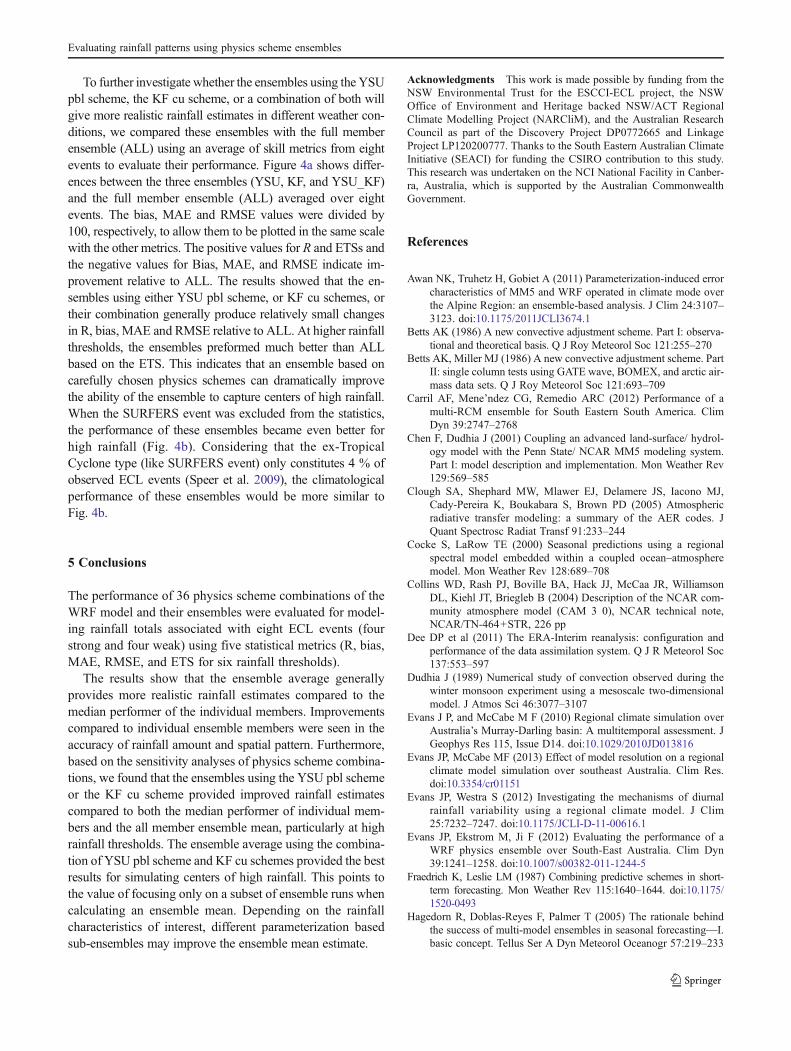
To further investigate whether the ensembles using the YSUpbl scheme, the KF cu scheme, or a combination of both willgive more realistic rainfall estimates in different weather con-ditions, we compared these ensembles with the full memberensemble (ALL) using an average of skill metrics from eightevents to evaluate their performance. Figure 4a shows differ-ences between the three ensembles (YSU, KF, and YSU_KF)and the full member ensemble (ALL) averaged over eightevents. The bias, MAE and RMSE values were divided by100, respectively, to allow them to be plotted in the same scalewith the other metrics. The positive values for R and ETSs andthe negative values for Bias, MAE, and RMSE indicate im-provement relative to ALL. The results showed that the en-sembles using either YSU pbl scheme, or KF cu schemes, ortheir combination generally produce relatively small changesin R, bias, MAE and RMSE relative to ALL. At higher rainfallthresholds, the ensembles preformed much better than ALLbased on the ETS. This indicates that an ensemble based oncarefully chosen physics schemes can dramatically improvethe ability of the ensemble to capture centers of high rainfall.When the SURFERS event was excluded from the statistics,the performance of these ensembles became even better forhigh rainfall (Fig. 4b). Considering that the ex-TropicalCyclone type (like SURFERS event) only constitutes 4 % ofobserved ECL events (Speer et al. 2009), the climatologicalperformance of these ensembles would be more similar toFig. 4b.

5 Conclusions

The performance of 36 physics scheme combinations of theWRF model and their ensembles were evaluated for model-ing rainfall totals associated with eight ECL events (fourstrong and four weak) using five statistical metrics (R, bias,MAE, RMSE, and ETS for six rainfall thresholds).

The results show that the ensemble average generallyprovides more realistic rainfall estimates compared to themedian performer of the individual members. Improvementscompared to individual ensemble members were seen in theaccuracy of rainfall amount and spatial pattern. Furthermore,based on the sensitivity analyses of physics scheme combina-tions, we found that the ensembles using the YSU pbl schemeor the KF cu scheme provided improved rainfall estimatescompared to both the median performer of individual mem-bers and the all member ensemble mean, particularly at highrainfall thresholds. The ensemble average using the combina-tion of YSU pbl scheme and KF cu schemes provided the bestresults for simulating centers of high rainfall. This points tothe value of focusing only on a subset of ensemble runs whencalculating an ensemble mean. Depending on the rainfallcharacteristics of interest, different parameterization basedsub-ensembles may improve the ensemble mean estimate.

Acknowledgments This work is made possible by funding from theNSW Environmental Trust for the ESCCI-ECL project, the NSWOffice of Environment and Heritage backed NSW/ACT RegionalClimate Modelling Project (NARCliM), and the Australian ResearchCouncil as part of the Discovery Project DP0772665 and LinkageProject LP120200777. Thanks to the South Eastern Australian ClimateInitiative (SEACI) for funding the CSIRO contribution to this study.This research was undertaken on the NCI National Facility in Canber-ra, Australia, which is supported by the Australian CommonwealthGovernment.

References

Awan NK, Truhetz H, Gobiet A (2011) Parameterization-induced errorcharacteristics of MM5 and WRF operated in climate mode overthe Alpine Region: an ensemble-based analysis. J Clim 24:3107–3123. doi:10.1175/2011JCLI3674.1

Betts AK (1986) A new convective adjustment scheme. Part I: observa-tional and theoretical basis. Q J Roy Meteorol Soc 121:255–270

Betts AK, Miller MJ (1986) A new convective adjustment scheme. PartII: single column tests using GATE wave, BOMEX, and arctic air-mass data sets. Q J Roy Meteorol Soc 121:693–709

Carril AF, Mene’ndez CG, Remedio ARC (2012) Performance of amulti-RCM ensemble for South Eastern South America. ClimDyn 39:2747–2768

Chen F, Dudhia J (2001) Coupling an advanced land-surface/ hydrol-ogy model with the Penn State/ NCAR MM5 modeling system.Part I: model description and implementation. Mon Weather Rev129:569–585

Clough SA, Shephard MW, Mlawer EJ, Delamere JS, Iacono MJ,Cady-Pereira K, Boukabara S, Brown PD (2005) Atmosphericradiative transfer modeling: a summary of the AER codes. JQuant Spectrosc Radiat Transf 91:233–244

Cocke S, LaRow TE (2000) Seasonal predictions using a regionalspectral model embedded within a coupled ocean–atmospheremodel. Mon Weather Rev 128:689–708

Collins WD, Rash PJ, Boville BA, Hack JJ, McCaa JR, WilliamsonDL, Kiehl JT, Briegleb B (2004) Description of the NCAR com-munity atmosphere model (CAM 3 0), NCAR technical note,NCAR/TN-464+STR, 226 pp

Dee DP et al (2011) The ERA-Interim reanalysis: configuration andperformance of the data assimilation system. Q J R Meteorol Soc137:553–597

Dudhia J (1989) Numerical study of convection observed during thewinter monsoon experiment using a mesoscale two-dimensionalmodel. J Atmos Sci 46:3077–3107

Evans J P, and McCabe M F (2010) Regional climate simulation overAustralia’s Murray-Darling basin: A multitemporal assessment. JGeophys Res 115, Issue D14. doi:10.1029/2010JD013816

Evans JP, McCabe MF (2013) Effect of model resolution on a regionalclimate model simulation over southeast Australia. Clim Res.doi:10.3354/cr01151

Evans JP, Westra S (2012) Investigating the mechanisms of diurnalrainfall variability using a regional climate model. J Clim25:7232–7247. doi:10.1175/JCLI-D-11-00616.1

Evans JP, Ekstrom M, Ji F (2012) Evaluating the performance of aWRF physics ensemble over South-East Australia. Clim Dyn39:1241–1258. doi:10.1007/s00382-011-1244-5

Fraedrich K, Leslie LM (1987) Combining predictive schemes in short-term forecasting. Mon Weather Rev 115:1640–1644. doi:10.1175/1520-0493

Hagedorn R, Doblas-Reyes F, Palmer T (2005) The rationale behindthe success of multi-model ensembles in seasonal forecasting—I.basic concept. Tellus Ser A Dyn Meteorol Oceanogr 57:219–233

Evaluating rainfall patterns using physics scheme ensembles

Hong S-Y, Lim J-OJ (2006) The WRF single-moment 6-class micro-physics scheme (WSM6). J Kor Meteor Soc 42:129–151

Hong S-Y, Dudhia J, Chen S-H (2004) A revised approach to icemicrophysical processes for the bulk parameterization of cloudsand precipitation. Mon Weather Rev 132:103–120

Hong SY, Noh Y, Dudhia J (2006) A new vertical diffusion packagewith an explicit treatment of entrainment processes. Mon WeatherRev 134:2318–2341

Ishizaki Y, Nakaegawa T, Takayabu I (2012) Validation of precipitationover Japan during 1985–2004 simulated by three regional climatemodels and two multi-model ensemble means. Clim Dyn 39:185–206

Janjic ZI (1994) The step-mountain eta coordinate model: further de-velopments of the convection, viscous sublayer and turbulenceclosure schemes. Mon Weather Rev 122:927–945

Janjic ZI (2000) Comments on “Development and evaluation of aconvection scheme for use in climate models”. J Atmos Sci57:3686

Jankov I, Gallus W Jr, Segal M, Shaw B, Koch S (2005) The impact ofdifferent WRF model physical parameterizations and their inter-actions on warm season MCS rainfall. Weather Forecast 20:1048–1060

Jones D, Wang W, Fawcett R (2009) High-quality spatial climate data-sets for Australia. Aust Meteorol Mag 58:233–248

Kain JS (2004) The Kain-Fritsch convective parameterization: anupdate. J Appl Meteorol 43:170–181

Kain JS, Fritsch JM (1990) A one-dimensional entraining/ detrainingplume model and its application in convective parameterization. JAtmos Sci 47:2784–2802

Kain JS, Fritsch JM (1993) Convective parameterization for mesoscalemodels: the Kain-Fritsch scheme, the representation of cumulusconvection in numerical models. In: Emanuel KA, Raymond DJ(eds) Amer Meteor Soc 246 pp

Mlawer EJ, Taubman SJ, Brown PD, Iacono MJ, Clough SA (1997)Radiative transfer for inhomogeneous atmosphere: RRTM, a val-idated correlated-k model for the long-wave. J Geophys Res102:16663–16682

Paulson CA (1970) The mathematical representation of wind speedand temperature profiles in the unstable atmospheric surface layer.J Appl Meteorol 9:857–861

Pepler AS, Rakich CS (2010) Extreme inflow events and synopticforcing in Sydney catchments. IOP Conf Ser: Earth Environ Sci(EES) 11(012010). doi:10.1088/1755-1315/11/1/012010

Phillips TJ, Gleckler PJ (2006) Evaluation of continental precipitationin 20th century climate simulations: the utility of multimodelstatistics. Water Resour Res 42(3). doi: 10.1029/2005WR004313

Schaller N, Mahlstein I, Cermak J, Knutti R (2011) Analyzing precip-itation projections: a comparison of different approaches to cli-mate model evaluation. J Geophys Res 116(10). doi:10.1029/2010JD014963

Schwartz CS, Kain JS, Weiss SJ, Xue M, Bright DR, Kong F, ThomasKW, Levit JJ, Coniglio MC, Wandishin MS (2010) Toward im-proved convection-allowing ensembles: model physics sensitivi-ties and optimizing probabilistic guidance with small ensemblemembership. Weather Forecast 25:263–280. doi:10.1175/2009WAF2222267.1

Skamarock WC, Klemp JB, Dudhia J, Gill DO, Barker DM, Duda M,Huang XY, Wang W, Powers JG (2008) A description of theadvanced research WRF version 3. NCAR, Boulder, NCARTechnical Note

Speer M, Wiles P, Pepler A (2009) Low pressure systems off the NewSouth Wales coast and associated hazardous weather: establish-ment of a database. Aust Meteorol Oceanogr J 58:29–39

Webb EK (1970) Profile relationships: the log-linear range, and exten-sion to strong stability. Q J Roy Meteorol Soc 96:67–90

Wilks DS (2006) Statistical methods in the atmospheric sciences, 2ndedn. Academic Press, Amsterdam, p 627, InternationalGeophysics Series, 91

Yuan X, Liang XZ (2011) Improving cold season precipitation predic-tion by the nested CWRF-CFS system. Geophys Res Lett 38,L02706. doi:10.1029/2010GL046104

Yuan X, Liang XZ, Wood EF (2012) WRF ensemble downscalingseasonal forecasts of China winter precipitation during 1982–2008. Clim Dyn 39:2041–2058. doi:10.1007/s00382-011-1241-8

F. Ji et al.