Journal of Biomolecular NMR, 20: 297–310, 2001.KLUWER/ESCOM© 2001 Kluwer Academic Publishers. Printed in the Netherlands.

297

Calculation of NMR-relaxation parameters for flexible molecules frommolecular dynamics simulations

Christine Peter, Xavier Daura & Wilfred F. van Gunsteren∗Laboratory of Physical Chemistry, Swiss Federal Institute of Technology Zürich, ETH-Zentrum, CH-8092 Zürich,Switzerland

Received 22 December 2000; Accepted 10 May 2001

Key words: internal dynamics, molecular dynamics simulation, NMR relaxation, NOESY, peptides, relaxationmatrix, ROESY, spectral density functions

Abstract

Comparatively small molecules such as peptides can show a high internal mobility with transitions between severalconformational minima and sometimes coupling between rotational and internal degrees of freedom. In those casesthe interpretation of NMR relaxation data is difficult and the use of standard methods for structure determination isquestionable. On the other hand, in the case of those system sizes, the timescale of both rotational and internalmotions is accessible by molecular dynamics (MD) simulations using explicit solvent. Thus a comparison ofdistance averages (〈r−6〉−1/6 or 〈r−3〉1/3) over the MD trajectory with NOE (or ROE) derived distances is nolonger necessary, the (back)calculation of the complete spectra becomes possible. In the present study we use two200 ns trajectories of a heptapeptide of β-amino acids in methanol at two different temperatures to obtain theoreticalROESY spectra by calculating the exact spectral densities for the interproton vectors and the full relaxation matrix.Those data are then compared with the experimental ones. This analysis permits to test some of the assumptions andapproximations that generally have to be made to interpret NMR spectra, and to make a more reliable predictionof the conformational equilibrium that leads to the experimental spectrum.

Introduction

In the standard methods of structure determinationbased on NMR relaxation data, interatomic distancesin a molecular model are compared to NMR-deriveddistances. The model can be a single structure or a setof structures, e.g., from a molecular dynamics (MD)simulation. In this case the interatomic distances in theset of structures are usually averaged according to themethod that describes best the relationship betweenfluctuating distances and NMR relaxation parameters,i.e. 〈r−6〉- or 〈r−3〉-averaging (Tropp, 1980).

This procedure is for two reasons problematic inthe case of small molecules that show a high internalmobility with transitions between several conforma-tional minima. First, the averaging method is not very

∗To whom correspondence should be addressed. E-mail:wfvgn@igc.phys.chem.ethz.ch

sensitive to distance fluctuations. A small fraction ofstructures with short distances between two atoms canmake a large contribution to the average, so that alarger fraction of structures with longer distances canbe hidden or at least underestimated (Daura et al.,1999a; Bürgi et al., 2001). Second, the interatomicdistances and their fluctuations are not the only quan-tities which determine NMR relaxation rates and thus,for example, ROESY crosspeak intensities, but thereis also an additional contribution from intramolecu-lar motions to the observed signal by their timescalesand their orientational correlations. This contributionis usually neglected or implicitly included using themodel-free approach by Lipari and Szabo (1982). Thisis reasonable in the case of large and comparativelystiff molecules such as proteins, where the internal dy-namics is considerably faster than the overall tumbling(Lipari and Szabo, 1982).

298

Besides these difficulties, the comparison betweendistances is not really necessary for small molecules,because the whole timescale of both rotational and in-ternal motions is accessible via molecular dynamicssimulations even when using explicit solvent mole-cules. Thus, the (back)calculation of the relaxationparameters and of the complete 2D-NMR spectra ispossible.

In the present study, two 200 ns MD simulationsof a heptapeptide of β-amino acids in methanol at298 K and at 340 K (Daura et al., 1998, 1999b) areanalyzed. The correlation times and order parametersfor rotational and internal motions are investigated indetail, as well as possible couplings between tumblingand internal dynamics. Theoretical ROESY spectra forboth trajectories are computed. The influence of thevarious aspects of internal dynamics (distance fluctu-ations, timescales, orientational correlations) on thecrosspeak intensities is tested, and the analysis showsthat it is possible to obtain additional information byconsidering not only distance averages but the com-plete dynamical information. Finally, the theoreticalROESY spectra and the buildup curves for selectedcrosspeaks are compared with values obtained fromexperimental spectra, leading to new observationsabout the folding/unfolding equilibrium in the probe.

Methods

Theoretical background

Because the major goal in this study is to calculateNOESY and ROESY spectra, all formulae presentedbelow are only given for the proton-proton dipolarinteraction. However, they can be easily adapted forother relaxation-inducing interactions such as chemi-cal shift anisotropy.

Time correlation functions and spectral densitiesNMR relaxation, i.e., the return of a spin systemto equilibrium, is determined by the transition prob-abilities between the energy levels involved. Thesetransition probabilities depend on the fluctuations ofthe relaxation-inducing Hamiltonian and especially onthose frequency components of the fluctuations thatcorrespond to the transition frequency. The Hamil-tonian that describes the spin system can be separatedinto two terms, spin operator functions and spacialfunctions, the latter containing all temporal fluctua-tions. For the dipolar interaction of two spins I and

S, the Hamiltonian is given by

H (t) = µ0

4π

γ2h2

r3(t)

(I(t) · S(t)

− 3

r2(t)(I(t) · r(t))(S(t) · r(t))

)(1)

= µ0

4π

γ2h2

r3(t)

2∑m=−2

(−1)m Y2,−m(θ(t),

φ(t)) T2,m(I, S).

Here T2,m(I, S) are the second rank irreducible ten-sor spin-operators and Y2,−m(θ,φ) are the secondrank spherical harmonic functions (Tropp, 1980). r(t)is the internuclear vector and θ(t) and φ(t) are itstime-dependent polar angles in a laboratory frame ofreference. γ is the gyromagnetic ratio of the proton,h is Planck’s constant divided by 2π and µ0 is thepermeability of free space. As shown elsewhere (Ap-pendix of Neuhaus and Williamson (1989) or Fischeret al. (1998)) transition probabilities, and thus relax-ation rates, are determined by the discrete Fourier-coefficients of time-correlation functions Cmn(τ) ofthe spherical harmonics involved in Equation 1

Cmn(τ)=4π

⟨Y2,m(θ(t),φ(t)) Y2,n(θ(t + τ),φ(t + τ))

r3(t) r3(t + τ)

⟩.

(2)

Spectral-density functions Jmn(ω) are the Fourier-transforms of these time-correlation functions

Jmn(ω) =∫ ∞

−∞Cmn(τ) e−iωτ dτ. (3)

In the following only terms of Cmn(τ) with m = n

are needed. Furthermore is Cmm(τ) in an isotropic liq-uid invariant under rotation of the laboratoy frame. Itcan be shown that therefore Cmm is independent ofm (Brüschweiler and Case, 1994). Summing over m

and using the following addition theorem for sphericalharmonics

2∑m=−2

Y2,m(θ(t),φ(t))Y∗2,m(θ(t + τ),φ(t + τ)) =

5

4πP2(cos χt,t+τ), (4)

where P2(x) = 32x

2 − 12 is the second-order Legendre

polynomial and χt,t+τ is the angle between the inter-spin vector at the two timepoints t and t + τ, gives

299

the following formula for the time-correlation functionthat determines relaxation

C(τ) = 1

5

2∑m=−2

Cmm(τ) =⟨P2(cos χt,t+τ)

r3(t) r3(t + τ)

⟩. (5)

In the following, only this time-correlation functionand its Fourier-transform J (ω) will be used.

An alternative, equivalent description of the inter-action Hamiltonian (see Equation 1) is

H = −µ0

4πγ2 h2 I · D(t) · S, (6)

where

D(t) = 1

r5

3x2 − r2 3xy 3xz

3yx 3y2 − r2 3yz3zx 3zy 3z2 − r2

(7)

is the dipole-dipole interaction tensor. This form is of-ten computationally more convenient because it relieson cartesian coordinates instead of spherical harmon-ics. The correlation functions of the tensor elements(only five are independent because D(t) is symmetricand traceless) are equivalent to those of the sphericalharmonics. Again, in an isotropic liquid all auto- andcross-correlation functions of the matrix elements areeither equal (except for some constant scaling factors)or zero (H.J.C. Berendsen, personal communication),and the averaging over all nine matrix-element corre-lation functions is equal to the averaging in Equation4. This second approach will be mainly used wheremodels for some internal motions have to be includedand a straightforward use of the second Legendre poly-nomial as in Equation 5 is impossible, e.g., in the caseof the united-atom methyl-groups as described below.

Dipolar relaxation in a two-spin systemIn a system of two protons i and j the longitudinalrelaxation of each proton is given by

d(Iz(t) − I0)i

dt= −ρij (Iz(t) − I0)i

− σij (Iz(t) − I0)j . (8)

Here, (Iz(t) − I0)i is the deviation of the ‘magnetiza-tion’ (the z component expectation value of the spinoperator of spin i) from its equilibrium value, ρij isthe direct dipolar relaxation rate constant of spin i

by spin j , and σij is the cross-relaxation rate. Theserelaxation rates, which control the magnitude of anNOE enhancement and the intensity of the signalsin a NOESY spectrum, are given by the following

formulae (Neuhaus and Williamson, 1989)

ρij = 110K

2 (3 J (2ω0) + 32J (ω0) + 1

2J (0))

(NOESY) (9)

σij = 110K

2 (3 J (2ω0) − 12 J (0)

), (10)

J (ω) being spectral-density functions of the inter-spin vector, ω0 the Larmor frequency of the protons,and K = (µ0/4π)hγ2. In the case of a rigid mole-cule which tumbles isotropically according to Brown-ian motion, the time-correlation function is a singleexponential function with a correlation time τc

C(τ) = 1

r6ij

e−τ/τc (11)

and

J (ω) = 1

r6ij

2 τc

1 + ω2τ2c

, (12)

rij being the interspin distance.Due to the minus sign in Equation 10, the cross-

relaxation rate changes sign for tumbling rates with

ω0τc =√

54 ≈ 1, and therefore, the NOESY cross-

peak intensity can come close to zero depending onthe tumbling rate of the molecule. In this case, rotat-ing frame experiments (ROESY) are performed wherethis zero-transition does not occur. Then, the measuredintensities are determined by the following relaxationrates (K as defined above) (Neuhaus and Williamson,1989):

ρ = 110K

2 ( 32 J (2ω0) + 9

4 J (ω0) + 54 J (0)

)(ROESY), (13)

σ = 110K

2 ( 32 J (ω0) + J (0)

)(14)

Multispin systems and the relaxation matrixIn the case of a system of n spins, a set of coupleddifferential equations similar to Equation 8 describesthe magnetization ot the individual spins:

d(Iz(t) − I0)i

dt= −ρi (Iz(t) − I0)i −

−n∑

j=1, �=i

σij (Iz(t) − I0)j .

(15)

Here ρi = ∑nj=1, �=i ρij + L1,i is the total longitudi-

nal relaxation rate of spin i with the ‘leakage’ L1,i ,i.e., relaxation due to other relaxation mechanisms,such as chemical shift anisotropy, and intermolecu-lar dipole-dipole relaxation by paramagnetic species

300

such as dissolved oxygen. This additional contribu-tion is unfortunately hard to estimate and can onlyapproximately be included into the calculations.

The isolated-spin-pair approach, in which a cross-peak intensity is given directly by the cross relaxationrate of the corresponding spin-pair, is only as a first-order approximation applicable. In most cases theso-called ‘spin-diffusion’ is not negligible, i.e., thecoupled system of Equations 15 has to be solved(Macura and Ernst, 1980; Keepers and James, 1984;Boelens et al., 1989). The equations can be rewrittenin the matrix form

dM(t)

dt+ R M(t) = 0 (16)

with

Mii(t) = (Iz(t) − I0)i (17)

Mij(t) = 0 for i �= j (18)

Rii = ρi (19)

Rij = σij. (20)

Here, M(tm) is the matrix with the intensities of theNOESY- (or ROESY-)spectrum after a mixing time tm.M(0), the spectrum at mixing time ‘zero’, contains theintensities of the 1D-spectrum along the diagonal.

The matrix Equation 16 may be solved by diago-nalization of the relaxation matrix R, leading to thesolution

M(tm) = X e−�tm X−1 M(0), (21)

where � = X−1RX contains the eigenvalues of Ras diagonal elements, and X is the correspondingeigenvector matrix.

Methyl groups – a slight complicationIn many MD simulations protons that are bound to analiphatic carbon atom are, together with that carbon,incorporated into a united atom to save computationaleffort. In the case of methyl groups this has the effectthat the exact positions of the three protons are notknown but only their positional average. Thus, modelsfor the methyl rotation have to be used to describe therelaxation of proton pairs where one or both protonsare members of methyl groups.

One model for methyl-group rotation is a three-site jump described in (Tropp, 1980). Here, the threepossible vectors connecting a nonmethyl proton tothe positions of the methyl protons are evaluated (re-spectively the nine vectors in case of the interactionbetween two methyl groups) and an averaging over

the spherical harmonics of the N (N = 3 or 9) in-teraction vectors is performed before the correlationfunction of the spherical harmonics is calculated ac-cording to Equation 2. This is more conveniently donein Cartesian space by calculating the five indepen-dent elements of matrix D (see Equation 7) for the N

vectors

Cij(τ) =⟨(

N∑k=1

Dij,k(t)

)(N∑k=1

Dij,k(t + τ)

)⟩

1 ≤ i, j ≤ 3; N = 3 or 9. (22)

Here N = 3 or 9 is the number of different in-teraction vectors and Dij,k is the element ij of Dcorresponding to the kth interaction vector. To obtainthe optimal statistics over all orientations in space, av-eraging equivalent to Equations 4 and 5 is performed(the prefactor 1

6 = Tr(r3 · D)2 was chosen to obtainthe same scaling as in Equation 5)

C(τ) = 1

6

3∑i,j=1

Cij. (23)

In this treatment the correlation time of the methyl-group rotation is not included. In principle this is onlycorrect if this rotation is much faster than the other mo-tions in the system (Edmondson, 1994), which mightbe problematic for small molecules like peptides, butshould not qualitatively change the results.

One term that should still be added is the intra-methyl-group relaxation. It gives an additional contri-bution to the diagonal elements of R if i is a methylgroup. The spectral density functions for interactionsbetween two protons in the same methyl group are(Edmondson, 1992; Woessner, 1962)

J (ω) = 1

r6m

(1

4

τc

1 + ω2τ2c

+ 3

4

τa

1 + ω2τ2a

), (24)

1

τa= 1

τc+ 1

τm, (25)

where τm is the correlation time of the methyl-grouprotation and rm is the distance between the two pro-tons. The values τm = 0.1 ns and rm = 0.17 nm werechosen according to (Edmondson, 1992).

An additional complication is that a methyl groupis treated as a single site in the relaxation and the mag-netization matrix, i.e., in the expression (Iz − I0)i themagnetization of the three protons has been summedif i is a methyl group. As a consequence R becomesnonsymmetric because σij = 3 σji if i is a methylgroup and j is a nonmethyl proton, as can be seen from

301

Equation 15. This problem can be solved by makingR symmetric before diagonalizing it, as described in(Olejniczak, 1989).

Computation of the spectra

The computation of NOESY or ROESY spectra wasdone in a three-step procedure in order to make it asflexible as possible. Because the calculation of time-correlation functions is computationally expensive, itwas done not for all proton pairs but only for a selected(significant) subset:1. Those proton pairs were selected which were ei-

ther close or for which the distance fluctuatedsignificantly:

〈r−6〉−16

traj ≤ MAXDIST or

(〈r2〉traj − 〈r〉2traj)

12 /〈r〉traj ≥ MINFLUC

The subscript traj indicates an average over thewhole MD trajectory. For the β-heptapeptide test-system the criteria MAXDIST = 0.4 nm andMINFLUC = 0.4 were chosen, so that all long-distance NOEs measured experimentally were ex-plicitly calculated.

2. The time-correlation and spectral-density func-tions of the interproton vectors of the selected pairswere computed according to Equation 5 or 22 and23.

3. A relaxation matrix for a rigidly tumbling mole-cule was computed using Equation 12. The val-ues of the spectral densities of the selected pairswere substituted by those that had been calculatedexplicitly in step 2. After symmetrizing and di-agonalizing the relaxation matrix the theoreticalspectrum was obtained. For the distances needed inEquation 12, 〈r−6〉−1/6-distance averages from aset of structures were used. This set included eitherthe whole trajectory (〈r−6〉−1/6

traj ) or structures thatwere representative for a specific conformation(〈r−6〉−1/6

conf ).

Results and discussion

A detailed description of the MD simulations of theβ-heptapeptide in methanol at 298 K and at 340 K isgiven by Daura et al. (1998, 1999b). At 298 K thesystem is found mainly (≈ 95% of the simulation) inthe folded conformation, which is a left-handed 314-helix. In the 340 K simulation the system spends only36% of the time in the folded state, folding/unfolding

occurring on a timescale of about 10 ns. Although at340 K the system is more than 50% of the time in con-formations that deviate considerably from the NOE-derived model structure, the trajectory-averages of theinterproton distances still satisfy quite well the NOEdistance restraints (Daura et al., 1999a). Therefore,comparison of average distances from a simulationwith experimentally derived distances is not a veryreliable criterium to investigate the folding/unfoldingequilibrium of a peptide.

A model of the folded conformation of the peptideis displayed in Figure 1. Additionally some vectorsthat will be frequently referred to later are indicated.From the 200 ns trajectories at 298 K and 340 Kstructures were saved every ps for the preliminaryanalysis of the system dynamics. The calculation ofROESY spectra was performed with peptide configu-rations that were saved every 5 ps. Before, tests hadshown that a more frequent saving of conformations(every 2 ps) would not alter the results.

Preliminary analysis of the system dynamics

Before calculating the NMR relaxation parametersof the system, a general analysis of the overall andinternal system dynamics was performed for both sim-ulations in order to get an answer to the followingquestions:

1. In which timescales do internal dynamics andoverall tumbling take place?

2. Is the overall tumbling isotropic?3. To which extent are internal dynamics and overall

tumbling correlated?Normalized time-correlation functions of the motionalprocesses of selected interatomic vectors were calcu-lated according to

C(τ) =⟨r−6(t)

⟩−1⟨P2(cos χt,t+τ)

r3(t) r3(t + τ)

⟩(26)

both with and without fitting the structures to a (he-lical) reference configuration. For the fitting a trans-lation of the center of mass to the origin followed bya rotational fit minimizing the root-mean-square po-sitional deviation of backbone atoms was performed.With this method the time correlation functions ofall motions in the laboratory frame, Call(τ), as wellas those of the internal motions in a molecule-fixedframe, Cint(τ), could be obtained. By calculating thetime correlation functions of the three orthonormalrow vectors of the rotation matrix that resulted fromthe fitting, the rotational time correlation function forthree directions, Crot(τ), could also be obtained.

302

Figure 1. Chemical structure and model helix of the β-heptapeptide with some vectors indicated; dashed lines: some long distance NOEs thatare typical for the helical structure (see also Figure 6); solid lines: two vectors (residue 3: Cβ – Cδ; residue 7: N-C(carbonyl)) for which a

preliminary analysis of the occurring motional processes was performed. Note that in the simulation the N-terminus was protonated (NH+3 ).

In the case of the three rotational time correlationfunctions the correlation times were determined by fit-ting a single exponential to Crot(τ). As in all othercases the decay of the correlation functions was non-exponential, a generalized order-parameter S2 and anestimate of the correlation time τcorr were determinedvia

S2 = limτ→∞C(τ) (27)

τcorr = 1

C(0) − S2

∫ tint

0(C(τ) − S2) dτ, (28)

where the integration limit tint was chosen as the firsttimepoint where the correlation function had reachedthe value of S2.

If internal and overall rotational motion were un-correlated and the overall tumbling corresponded toBrownian motion the following Equation should hold

Call(τ) ≈ Crot(τ)Cint(τ) = e−τ/τcCint(τ), (29)

where τc is the correlation time of the overall rotation.

Table 1. Rotational correlation times

T (K) τc – three directions (ps) Average (ps)

298 153 143 158 ≈ 150

340 74 76 75 ≈ 75

Additionally to the complete internal dynamics,the motions of the individual sidechains were inves-tigated by translating in each case the correspondingβ-carbon atom to the origin and performing a rota-tional fit based on the three atoms directly bonded tothe β-carbon atom.

The results for the rotational motion can be seen inTable 1. The overall tumbling is found to be approx-imately isotropic and has an average correlation timeof about 150 ps for the 298 K simulation and 75 ps forthe 340 K simulation. The rotational correlation timeof the molecule in the simulation at 298 K is prob-ably underestimated. It is known experimentally thatthe NOESY intensity at 500 MHz is approximately

303

Table 2. Order parameters S2 (Equation 27) and correlation times τ (Equation 28) of vectors in thethird and in the last residue. The subscript all refers to inclusion of all motions, int to internal motions(overall translation and rotation removed); the subscript COM refers to a translational/rotational fitaround the center of mass and therefore represents all internal motions, the subscript SC refers to atranslational/rotational fit around the Cβ-atom and therefore represents the sidechain motions

Vector T (K) τall (ps) τint,COM (ps) τint,SC (ps) S2int,COM S2

int,SC

C3β

– C3δ

298 94 126 206 0.57 0.65

C3γ – C3

δ298 66 140 63 0.30 0.36

C3γ – C3

ε 298 61 99 101 0.29 0.32

C3δ

– C3ε 298 47 63 41 0.21 0.24

C3β

– C3δ

340 44 1077 19 0.19 0.67

C3γ – C3

δ340 30 270 17 0.09 0.38

C3γ – C3

ε 340 25 332 15 0.04 0.32

C3δ

– C3ε 340 17 212 12 0.03 0.20

N7 – C7δ

298 84 646 287 0.27 0.68

N7 – C7(carbonyl) 298 105 1229 1882 0.29 0.68

N7 – C7δ

340 31 170 438 0.05 0.59

N7 – C7(carbonyl) 340 39 190 442 0.04 0.54

zero. According to Equation 10 combined with 12 thiszero transition should occur for correlation times ofroughly 360 ps. The fact that the rotational diffusionis too fast is not completely unexpected, because itis known that the diffusion constant for the methanolmodel used is also too large (Walser et al., 2000).

Correlation times of all motions, as well as cor-relation times and order parameters of the completeinternal dynamics and of the motions in the sidechains,are presented in Table 2 for vectors in the third and inthe last residue. If no addional types of motions appearat the higher temperature, correlation times are ex-pected to decrease with increasing temperature. Thisis the case for the last residue, which is never stronglyfixed in the helical secondary structure. However, theinternal correlation times of vectors in the third residueincrease with increasing temperature, which indicatesthat an additional, comparatively slow component isadded to the internal dynamics. This behaviour cannotbe observed for the internal motions of the sidechainsonly, which is to be expected because these sidechainrotations and vibrations should already be expressedat the lower temperature. These observations are con-firmed by the order parameters. S2

int,SC, the orderparameter of the sidechain motion, does hardly changewith temperature, while S2

int,COM, the order parameterof the complete internal motion, decreases stronglywith increasing temperature for both residues. In thecase of the third residue, both order parameters arevery similar at 298 K, indicating that the sidechain

fluctuations are the major component of the internaldynamics in this part of the molecule, whereas at340 K S2

int,COM is much smaller than S2int,SC. The lat-

ter observation holds for both temperatures in case ofthe terminal residue which shows large conformationalchanges.

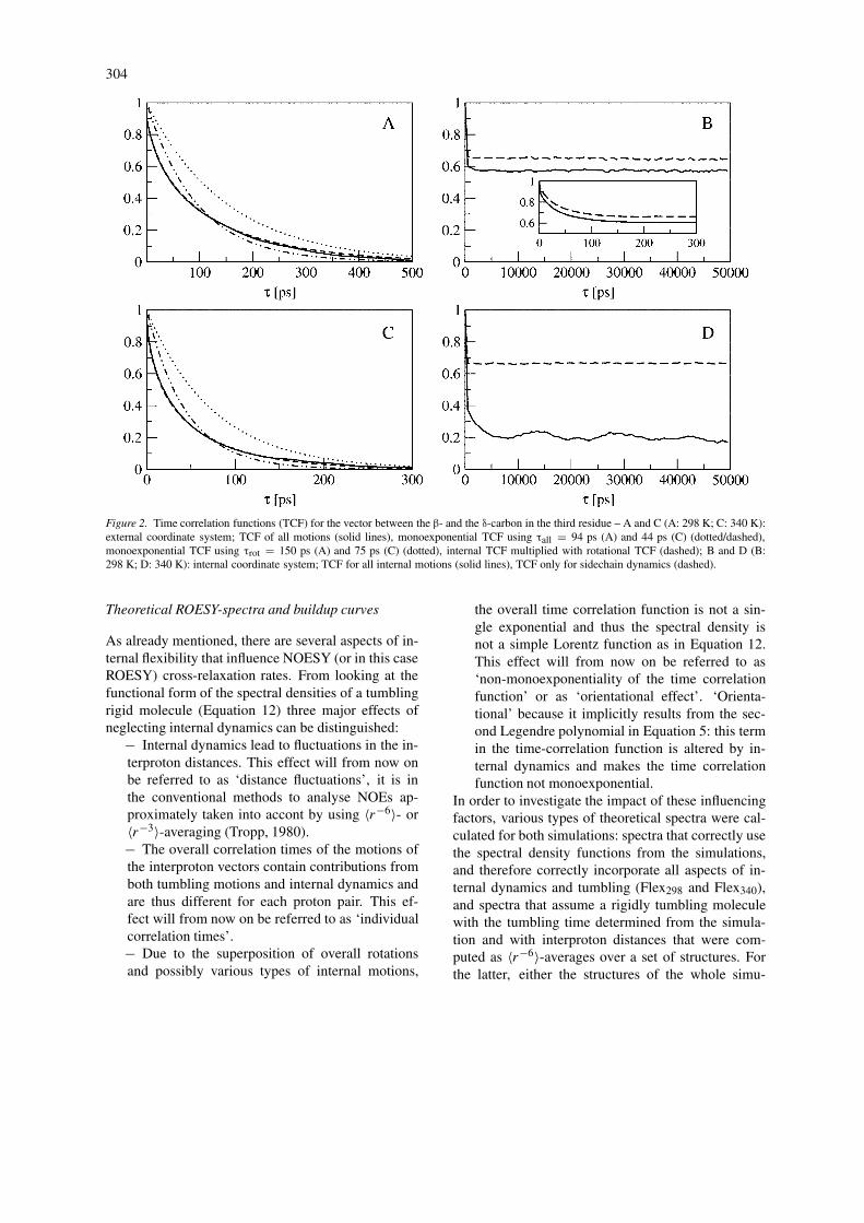
These results are illustrated in Figures 2 and 3where the various time correlation functions of tworepresentative vectors in these residues are shown. Forthe third residue (Figure 2) the product of the inter-nal time-correlation function with the exponential timecorrelation function of the tumbling (see Equation 29;dashed lines) matches the time correlation function ofall motions (solid lines) for both temperatures. Thus,the overall tumbling and the internal dynamics are notstrongly coupled for this residue. Equation 29 is lessaccurately satisfied in the case of the terminal residue(Figure 3). In all cases Call(τ) is not monoexponential,which implies that computing relaxation parameterswith a simple Lorentz function as in Equation 12 isnot sufficient.

The internal time correlation functions of theresidues that take part in helix formation show at340 K some periodicity with the approximate fre-quency of the folding and unfolding transitions. Thiseffect is absent at 298 K and in the case of the terminal(not helix forming) residue.

304

Figure 2. Time correlation functions (TCF) for the vector between the β- and the δ-carbon in the third residue – A and C (A: 298 K; C: 340 K):external coordinate system; TCF of all motions (solid lines), monoexponential TCF using τall = 94 ps (A) and 44 ps (C) (dotted/dashed),monoexponential TCF using τrot = 150 ps (A) and 75 ps (C) (dotted), internal TCF multiplied with rotational TCF (dashed); B and D (B:298 K; D: 340 K): internal coordinate system; TCF for all internal motions (solid lines), TCF only for sidechain dynamics (dashed).

Theoretical ROESY-spectra and buildup curves

As already mentioned, there are several aspects of in-ternal flexibility that influence NOESY (or in this caseROESY) cross-relaxation rates. From looking at thefunctional form of the spectral densities of a tumblingrigid molecule (Equation 12) three major effects ofneglecting internal dynamics can be distinguished:

− Internal dynamics lead to fluctuations in the in-terproton distances. This effect will from now onbe referred to as ‘distance fluctuations’, it is inthe conventional methods to analyse NOEs ap-proximately taken into accont by using 〈r−6〉- or〈r−3〉-averaging (Tropp, 1980).− The overall correlation times of the motions ofthe interproton vectors contain contributions fromboth tumbling motions and internal dynamics andare thus different for each proton pair. This ef-fect will from now on be referred to as ‘individualcorrelation times’.− Due to the superposition of overall rotationsand possibly various types of internal motions,

the overall time correlation function is not a sin-gle exponential and thus the spectral density isnot a simple Lorentz function as in Equation 12.This effect will from now on be referred to as‘non-monoexponentiality of the time correlationfunction’ or as ‘orientational effect’. ‘Orienta-tional’ because it implicitly results from the sec-ond Legendre polynomial in Equation 5: this termin the time-correlation function is altered by in-ternal dynamics and makes the time correlationfunction not monoexponential.

In order to investigate the impact of these influencingfactors, various types of theoretical spectra were cal-culated for both simulations: spectra that correctly usethe spectral density functions from the simulations,and therefore correctly incorporate all aspects of in-ternal dynamics and tumbling (Flex298 and Flex340),and spectra that assume a rigidly tumbling moleculewith the tumbling time determined from the simula-tion and with interproton distances that were com-puted as 〈r−6〉-averages over a set of structures. Forthe latter, either the structures of the whole simu-

305

Figure 3. Time correlation functions (TCF) for the vector between the nitrogen and the carbonyl carbon in the last residue – A and C (A:298 K; C: 340 K): external coordinate system; TCF of all motions (solid lines), monoexponential TCF using τall = 105 ps (A) and 39 ps (C)(dotted/dashed), monoexponential TCF using τrot = 150 ps (A) and 75 ps (C) (dotted), internal TCF multiplied with rotational TCF (dashed); Band D (B: 298 K; D: 340 K): internal coordinate system; TCF for all internal motions (solid lines), TCF only for sidechain dynamics (dashed).

lation (Rigtraj298 and Rigtraj

340) or a subset of structuresthat are representative for the helical conformation(Righelix

298 and Righelix340 ) were used. For this set, the con-

formations from the 340 K simulation were chosenwhich have a backbone-atom root-mean-square de-viation from the NMR model structure smaller than0.1 nm (Daura et al., 1999b). By looking at the rela-tive or the absolute differences between, for example,Rigtraj

340 and Flextraj340 the effects that do not stem from

‘distance fluctuations’ can be extracted. This allowsto test whether there is indeed a substantial neglect ofinformation when comparing only distance averagesfrom simulations and experimentally derived averagedistances.

The results are illustrated in Figure 4, where differ-ence spectra are plotted as matrices with the 50 protonsites ordered along the axes of the figures accordingto their sequence in the peptide. This sequence is foreach residue i: NiH, Ci

βH, sidechain protons from CiγH

to maximal CiεH, Ci

αHax and CiαHeq , the subscripts

ax and eq indicate the axial and equatorial positions

of the two Cα-protons in the model helix. Panel Ashows the relative difference between intensities ofall (cross)peaks in the ROESY spectra at 298 K fora rigid (trajectory average) and a flexible molecule,calculated using (Rigtraj

298 − Flextraj298)/Rigtraj

298. Panel Bshows the same for the 340 K simulation. To makesure that large relative differences between the spectraare really significant, the absolute difference is alsogiven for the simulation at 340 K (Rigtraj

340 − Flextraj340)

in panel C. Here the intensities were scaled such thatthey could be compared with experimentally measuredpeak volumes. The experimentally determined intensi-ties range from approximately 5 to 200 arbitrary units,which implies that matrix elements with a colour thatis different from dark blue in panel C denote a de-tectable difference in the spectra. As the main focusof this investigation is to study the effect of large con-formational changes of the peptide (mainly visible inthe behaviour of the backbone), backbone protons aremarked with coloured bars along the axes. Addition-ally some backbone proton pairs are highlighted with

306

Figure 4. Difference plots for theoretical ROESY spectra of theβ-heptapeptide (mixing time: 100 ms) between tumbling rigid(〈r−6〉-average over full trajectory) and flexible molecules; thenumbering of the protons follows the sequence in the peptide whichis for each residue i: NiH, Ci

βH, sidechain protons from Ci

γH to

maximal CiεH, Ci

αHax , CiαHeq ; coloured bars at the axes indicate

backbone protons (CiαHax , Ci

αHeq , Ni+1H and Ci+1β

H; red: i = 1,

blue: i = 2, green: i = 3, cyan: i = 5, yellow: i = 6, magenta: N5Hand C5

βH); white rings mark selected pairs of backbone protons – A:

298 K, relative difference; B: 340 K, relative difference; C: 340 K,absolute difference (arbitrary units which correspond to measuredpeak volumes – detectable intensities range from 5 to 200).

white circles. It can be observed that there is a changein the relative differences upon raising the tempera-ture from 298 K to 340 K, especially for those protonpairs which are in close proximity along the peptidebackbone, e.g., Ci

αHax – Ni+1H, NiH – CiαHax , Ci

βH

– Ni+1H. These are proton pairs where the ‘individualcorrelation times’ and the ‘orientational effects’ havea strong influence (in addition to the change in the dis-tance average) on the intensity of crosspeaks in case ofconformational fluctuations. It can also be seen, thatthese influences are not equally strong for all protonpairs. This can even lead to an inversion of the relativeintensity of two peaks depending on whether the inter-nal dynamics is treated exactly or only approximatelyvia distance averages (see below). Consequently in thecase of the simulation at 340 K where strong inter-nal dynamics occur, the explicit computation of thespectral density functions of individual proton pairsappears to be a requirement to reliably (back)calculateROESY spectra from MD simulations.

To monitor these effects in more detail theoreticalROESY-intensity buildup curves (i.e., crosspeak inten-sity as function of mixing time) of some selected pro-ton pairs were calculated. The results for both simu-lation temperatures and for all three above-mentionedcases (Righelix, Rigtraj and Flextraj) are shown in Fig-ure 5. Comparing Righelix

298 with Rigtraj298 and Righelix

340

with Rigtraj340 gives an impression how strongly the

‘fluctuating distances’ affect the intensities. Compar-ing these with Flextraj

298 and Flextraj340 permits assessing

all other additional effects included only by explicitcalculation of time correlation functions and spectraldensities, i.e., ‘individual correlation times’ and ‘non-monoexponentiality of the time correlation function’.As expected, the differences are rather small for thesimulation at 298 K, because the peptide is most ofthe time in the folded state. The situation is differentfor the simulation at 340 K. The ‘distance fluctua-tions’ can lead to a decrease or increase in the averagedistance resulting in an increase or decrease in in-tensity. This depends on whether the ‘collapse’ of arigid structure adds shorter distances to the averageand thus makes it smaller, or whether the breaking of arigid structure tears apart proton pairs which are keptclose, e.g., by hydrogen bonding, and thus leads toan increase in the average distance. Overall correla-tion times which include internal motions are usuallysmaller than the rotational correlation times only, sothat the ‘individual correlation times’ lead to a de-crease of intensity compared to a ‘rigid spectrum’.

307

Figure 5. Theoretical buildup curves – left panels (A and C) 298 K (τrot = 150 ps), right panels (B and D) 340 K (τrot = 75 ps); solid lines:

fully flexible molecule (Flextraj298 and Flextraj

340); dashed lines: rigid molecule, average over all conformations (Rigtraj298 and Rigtraj

340); dotted lines:

rigid molecule, average over helical structures (Righelix298 and Righelix

340 ); the proton pairs are indicated in the figure.

This decrease is of course individually strong, anddepends on the internal correlation time. The conse-quences for the relative intensities of a set of peaks ina spectrum can, for example, be seen in Figure 5 bycomparing the buildup curves of C2

αHax – C5βH, C5

βH

– N6H and N4H – C7βH.

By treating all internal motions explicitly, even the‘negative’ information that a signal is not observable

although it should be according to the distances in arigid structure, or that a peak is observable althoughthe interproton distance in a rigid structure would betoo big, can be used to analyse NOESY or ROESYspectra. Yet, it should be always kept in mind that‘leakage’ contributions to the longitudinal relaxationrate in Equation 15 cannot be calculated quantitativelyand may lead to artifacts.

308

Figure 6. Experimental and theoretical buildup curves – left (A and D): simulation at 298 K (Flextraj298), middle (B and E): experimental buildup

curves at 300 K, right (C and F): simulation at 340 K (Flextraj340) – upper panels (A–C): long distance backbone NOEs; lower panels (D–F): short

distance backbone NOEs – the proton pairs are indicated in the figure.

Comparison with experimental data

The theoretically calculated ROESY spectra from thetwo simulations can now be used to make a morereliable prediction of the ‘real’ folding/unfolding equi-librium of the β-heptapeptide. Experimental ROESYspectra at room temperature with mixing times of 50,100, 150 and 250 ms are available (Seebach et al.,1996). From these, a set of non-overlapping peakswas selected for which the intensities can be reliablydetermined by integration. To compare the buildup

curves of those experimental signals with the theoreti-cally calculated ones one scaling factor per simulationtemperature was determined by least-square fitting.Some of these buildup curves are shown exemplar-ily in Figure 6. The agreement between simulationand experiment for the long-distance (‘helical’) NOEs(upper panel) is reasonable but not excellent for bothsimulations, albeit still better for the simulation at 298K. However for NOEs that belong to backbone pro-ton pairs which are close in sequence (lower panel)

309

the agreement with experiment is clearly better forthe 298 K simulation compared to that for the 340 Ksimulation. This can be explained by the fact thatthe long-distance NOEs are probably mainly sensi-tive to the distance average and that the effects ofcorrelation times and the shape of the spectral den-sity functions (‘non-monoexponentiality of the timecorrelation function’) have a minor impact, whereasthey play a more important role for pairs which areseparated only by a few bonds.

Comparison of the curvatures of the experimentalbuildup curves with the ones from the simulation at298 K again indicates that the simulated correlationtimes are a bit too short, because an increase in thecorrelation times of all proton pairs shifts the maximaof the buildup curves towards shorter mixing times.

Besides these small discrepancies the results leadto the conclusion, that the simulation at 298 K givesa more realistic description of the true conforma-tional equilibrium of the peptide at room temperaturecompared to the simulation at 340 K.

Conclusions

Two 200 ns MD simulations of a β-heptapeptidetestsystem at 298 K and 340 K have been used toinvestigate the influence of internal flexibility of amolecule on NMR relaxation parameters. Various as-pects of the system dynamics have been considered(overall tumbling, internal motions, sidechain dynam-ics). The overall rotation of the molecules is foundto be essentially isotropic and the tumbling and inter-nal motions appear not to be coupled. The rotationalcorrelation times are approximately 150 ps and 75 psat 298 K and 340 K, respectively, which is too shortcompared to values indicated by NMR experimentsat room temperature. In the simulation at 298 K thepeptide stays most of the time in a folded (helical)conformation, and the internal dynamics is mainlyconfined to motions in sidechains and in the terminalresidues. In the simulation at 340 K several unfold-ing events and comparatively slow internal motionalprocesses occur. There are several reasons why thispeptide is a good testsystem to assess the advantagesof (back)calculating ROESY spectra compared to theconventional method of analysing ROESY spectra byonly comparing simulated distance averages with ex-perimentally derived average distances: it shows inter-nal fluctuations which have correlation times that areof the same order of magnitude or lower than the cor-

relation time of the overall tumbling, the correlationtimes of interatomic vectors are quite diverse, and thecorresponding time correlation functions are not sim-ply monoexponential. It could be shown, that internaldynamics have a strong influence on the cross-peak in-tensities of ROESY spectra. The explicit computationof spectral densities via the time correlation functionsof interproton vectors leads to significant differencesin the spectra compared to only calculating distanceaverages and neglecting possible other aspects of in-ternal dynamics, such as ‘individual correlation times’and ‘orientational effects’. This method makes the useof ‘negative’ information, i.e., the absence of specificcrosspeaks in the spectra, possible. Only the poten-tial influence of ‘leakage’ contributions from otherrelaxation mechanisms cannot be computed properly.

For the β-heptapeptide the comparison of theoreti-cal and experimental ROESY buildup curves suggeststhat the folding/unfolding equilibrium in the exper-iment lies more on the side of the folded (helical)state. This conclusion could hardly be made fromcomparing distance averages with ROE-derived dis-tances, as the experimentally derived distances werestill in good agreement with distance averages from asimulation with a 50/50 equilibrium distribution. Thisproves that it is possible to gain more informationabout the relationship between experiment and simula-tion by (back)calculating NMR spectra explicitly thanby comparing only distance averages.

For future applications this method of perform-ing unrestrained, explicit solvent MD simulations and(back)calculation of NMR relaxation parameters andspectra can be used in cases of even more flexiblemolecules, where no single configuration that satisfiesthe NOE derived distances can be found at all. Forsuch systems, where the interpretation of NMR dataalone seems to be a desperate venture because of theextreme internal mobility, this method could open newpossibilities to analyse structure and dynamics.

Acknowledgements

The authors wish to thank Prof. B. Jaun and co-workers for providing the ROESY spectra of theβ-heptapeptide and for giving a first introduction tospectra processing. Special thanks go to Prof. H.J.C.Berendsen for a number of helpful discussions aboutrotational averaging of tensors and suggestions espe-cially on the treatment of united-atom methyl groups.Financial support was obtained from the Schweiz-

310

erischer Nationalfonds, project number 21-50929.97,which is gratefully acknowledged.

References

Boelens, R., Koning, T.M.G., van der Marel, G.A., van Boom, J.H.and Kaptein, R. (1989) J. Magn. Reson., 82, 290–308.

Brüschweiler, R. and Case, D. (1994) Progr. NMR Spectrosc., 26,27–58.

Daura, X., Antes, I., van Gunsteren, W.F., Thiel, W. and Mark, A.E.(1999a) Proteins, 36, 542–555.

Daura, X., Jaun, B., Seebach, D., van Gunsteren, W.F. and Mark,A.E. (1998) J. Mol. Biol., 280, 925–932.

Daura, X., van Gunsteren, W.F. and Mark, A.E. (1999b) Proteins,34, 269–280.

Edmondson, S.P. (1992) J. Magn. Reson., 98, 283–298.

Edmondson, S.P. (1994) J. Magn. Reson., B103, 222–233.Fischer, M.W.F., Majumdar, A. and Zuiderweg, E.R.P. (1998) Progr.

NMR Spectrosc., 33, 207–272.Keepers, J.W. and James, T.L. (1984) J. Magn. Reson., 57, 404–426.Lipari, G. and Szabo, A. (1982) J. Am. Chem. Soc., 104, 4546–4559.Macura, S. and Ernst, R.R. (1980) Mol. Phys., 41, 95–117.Neuhaus, D. and Williamson, M. (1989) The Nuclear Overhauser

Effect in Structural and Conformational Analysis, VCH, NewYork, NY.

Olejniczak, E.T. (1989) J. Magn. Reson., 81, 392–394.Seebach, D., Ciceri, P.E., Overhand, M., Jaun, B., Rigo, D., Oberer,

L., Hommel, U., Amstutz, R. and Widmer, H. (1996) Helv. Chim.Acta, 79, 2043–2066.

Tropp, J. (1980) J. Chem. Phys., 72, 6035–6043.Walser, R., Mark, A.E., van Gunsteren, W.F., Lauterbach, M. and

Wipff, G. (2000) J. Chem. Phys., 112, 10450–10459.Woessner, D.E. (1962) J. Chem. Phys., 36, 1–4.