Caio A. S. CoelhoDepartment of Meteorology

University of Readingc.a.d.s.coelho@reading.ac.uk

Met Office, Exeter (U.K.), 20 February 2006

PLAN OF TALKCalibration and combination issuesConceptual framework for forecastingForecast Assimilation:

•Example 1: Nino-3.4 index forecasts•Example 2: Equatorial Pacific SST forecasts•Example 3: S. American rainfall forecasts•Example 4: Regional rainfall downscaling

EUROBRISA project

•

Forecast calibration and combination: Bayesian assimilation of

seasonal climate predictions

Thanks to: David B. Stephenson, Magdalena Balmaseda, Francisco J. Doblas-Reyes and Sergio Pezzulli

This talk is based on the following work: Coelho C.A.S. 2005: “Forecast Calibration and Combination: Bayesian Assimilation of Seasonal ClimatePredictions”. PhD Thesis. University of Reading. 178 pp.

Coelho C.A.S., D. B. Stephenson, M. Balmaseda, F. J. Doblas-Reyes and G. J. van Oldenborgh, 2005: Towards an integrated seasonal forecasting system for South America. ECMWF Technical Memorandum No. 461, 26pp. Also in press in the J. Climate.

Coelho C.A.S., D. B. Stephenson, F. J. Doblas-Reyes, M. Balmaseda, A. Guetter and G. J. vanOldenborgh, 2006: A Bayesian approach for multi-model downscaling: Seasonal forecasting of regionalrainfall and river flows in South America. Meteorological Applications, 13, 1-10.

Stephenson, D. B., Coelho, C. A. S., Doblas-Reyes, F.J. and Balmaseda, M., 2005: “Forecast Assimilation: A Unified Framework for the Combination of Multi-Model Weather and Climate Predictions.” Tellus A, Vol. 57, 253-264.

Coelho C.A.S., S. Pezzulli, M. Balmaseda, F. J. Doblas-Reyes and D. B. Stephenson, 2004: “Forecast Calibration and Combination: A Simple Bayesian Approach for ENSO”. Journal of Climate. Vol. 17, No. 7, 1504-1516.

Coelho C.A.S., S. Pezzulli, M. Balmaseda, F. J. Doblas-Reyes and D. B. Stephenson, 2003: “Skill of Coupled Model Seasonal Forecasts: A Bayesian Assessment of ECMWF ENSO Forecasts”. ECMWF Technical Memorandum No. 426, 16pp. Available from: http://www.met.rdg.ac.uk/~swr01cac

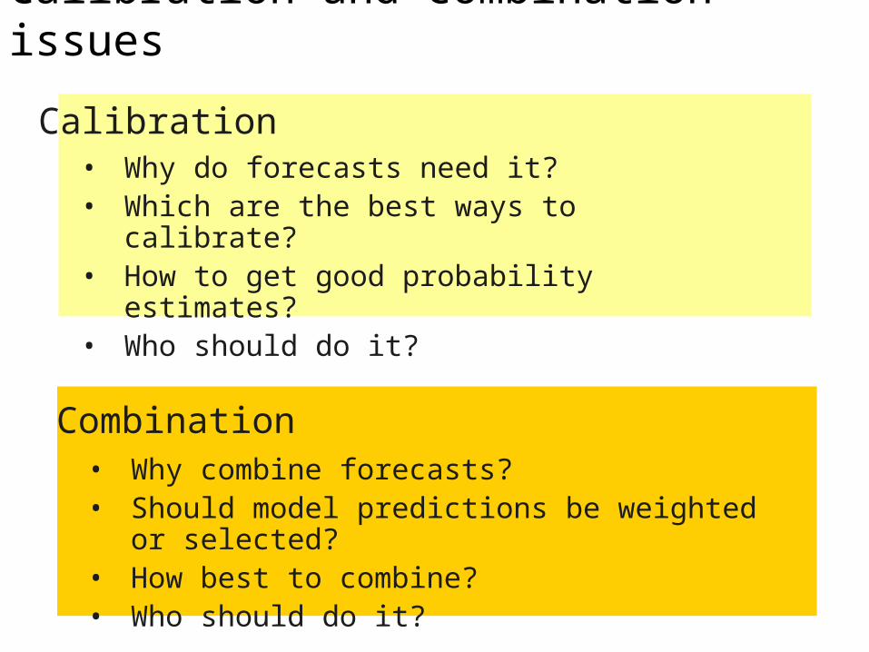
Calibration and combination issues

• Why do forecasts need it?• Which are the best ways to calibrate?• How to get good probability estimates?• Who should do it?

Calibration

Combination• Why combine forecasts?• Should model predictions be weighted or selected?• How best to combine?• Who should do it?

Conceptual framework

)y(p

)x(p)x|y(p)y|x(p

i

iiiii

Data Assimilation “Forecast Assimilation”

)x(p

)y(p)y|x(p)x|y(p

f

fffff

Multi-model ensemble approach

DEMETER DEMETER Development of a European Multi-Model Ensemble

System forSeasonal to Interannual Prediction

Solution: Multi-model Ensemble

Errors: Model formulationInitial conditions

http://www.ecmwf.int/research/demeter

DEMETER Multi-model ensemble system

7 coupled global circulation models

Hindcast period: 1980-2001 (1959-2001)

9 member ensembles

ERA-40 initial conditions

SST and wind perturbations

4 start dates per year

(Feb, May, Aug and Nov)

6 month hindcasts

Model Country

ECMWF International

LODYC France

CNRM France

CERFACS France

INGV Italy

MPI Germany

UKMO U.K.

.

.

..

Examples of application

•

• 0-d: Niño-3.4 index • 1-d: Equatorial Pacific SST• 2-d: South American rainfall

Example 1: Empirical Niño-3.4 forecasts

Well-calibrated: Most observations in the 95% prediction interval (P.I.)

95% P.I.valueJulyY

valueDecemberY

),Y(N~Y|Y

5t

t

2t05t1o5tt

ECMWF coupled model ensemble forecasts

Observations not within the 95% prediction interval! Coupled model forecasts need calibration

m=9DEMETER: 5-month

lead

2X

2ttt

2ttt sˆ;Xˆ);,(N~X

Prior:

Univariate X and Y

),(N~Y 2t0t0t

)V,Y(N~Y|X tttt

'

2X

t m

m

m

sV

),(N~X|Y 2tttt

t

t

2

2t0

t02

t

t

t

2

2t0

2t

X

V

V

11

)X(p

)Y(p)Y|X(p)X|Y(p

t

ttttt

Posterior:

Likelihood:

Bayes’ theorem:

Likelihood modelling:

y

t t t tX | Y ~ N( Y , V )

Combined forecasts

Note: most observations within the 95% prediction interval!

Comparison of the forecasts

Empirical Coupled

Combined SUMMARY

Combined forecasts:• are better calibrated than coupled• have less spread than empirical• match obs better than either

Blue dots = observationsRed dots = mean forecastGrey shade = 95% prediction interval

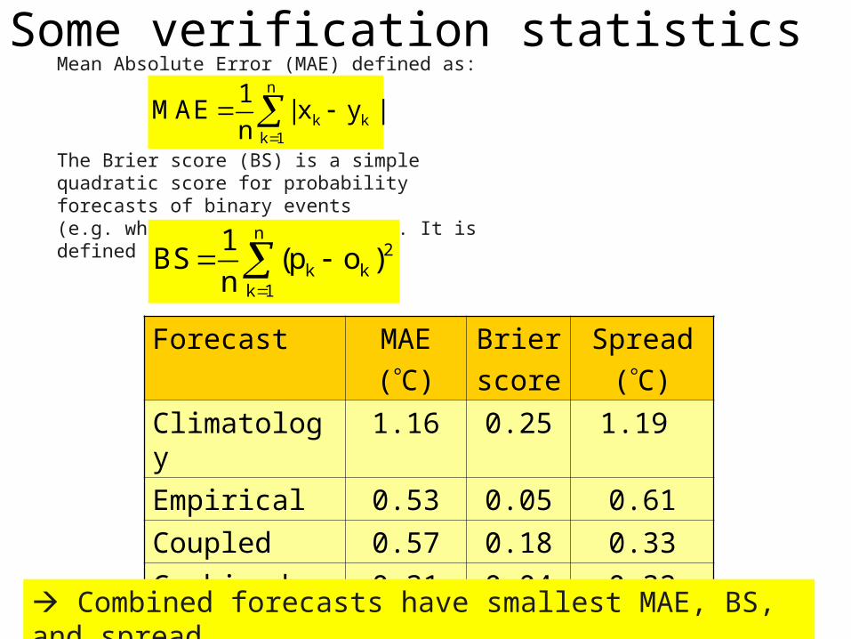
Mean Absolute Error (MAE) defined as:

The Brier score (BS) is a simple quadratic score for probability forecasts of binary events(e.g. whether SST anomaly < 0). It is defined as:

Some verification statisticsn

k kk 1

1MAE | x y |

n

n2

k kk 1

1BS (p o )

n

Forecast MAE

(C)

Brier

score

Spread

(C)

Climatology 1.16 0.25 1.19

Empirical 0.53 0.05 0.61

Coupled 0.57 0.18 0.33

Combined 0.31 0.04 0.32

Combined forecasts have smallest MAE, BS, and spread

)C,Y(N~Y b

1TT

111T

obba

)SGCG(CGL

C)LGI()CGSG(D

)]YY(GX[LYY

)S],YY[G(N~Y|X o

Prior:

Likelihood:

Posterior:

1YYXYSSG

YGXGYo T

YYXX GGSSS

)D,Y(N~X|Y a

Multivariate X and Y: More than one Normal variable

qq:D

qn:Y

pn:X

qq:C q1:Yb

pp:S qn:Ya

Matrices

Example 2: Equatorial Pacific SST

Forecast Brier Score

Climatol p=0.5 0.25

Multi-model 0.19

FA 58-01 0.17

)0YPr(p tt

SST anomalies: Y (°C)Forecast probabilities: p

DEMETER: 7 coupled models; 6-month lead

Y 0Y

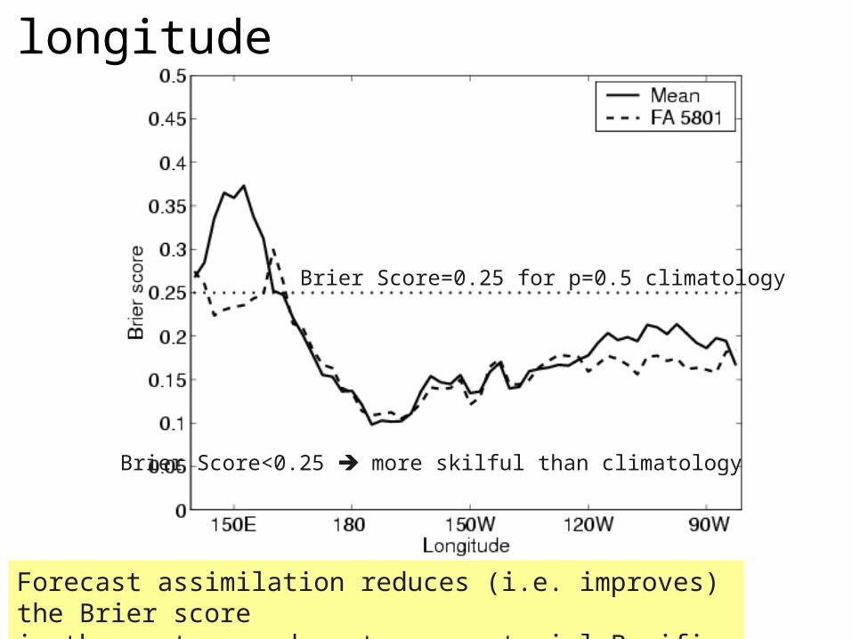
Forecast assimilation reduces (i.e. improves) the Brier score in the eastern and western equatorial Pacific

1BS0)op(n

1BS

n

1k

2kk

Brier Score as a function of longitude

Brier Score=0.25 for p=0.5 climatology

Brier Score<0.25 more skilful than climatology

Brier Score decomposition

1BS0)op(n

1BS

n

1k

2kk

)o1(o)oo(Nn

1)op(N

n

1BS

l

1i

2ii

l

1i

2iii

iNk

ki

i1i oN

1)p|o(po

n

1kko

n

1o

reliability resolution uncertainty

Forecast assimilation improves reliability in the western Pacific

Reliability as a function of longitude

Resolution as a function of longitude

Forecast assimilation improves resolution in the eastern Pacific

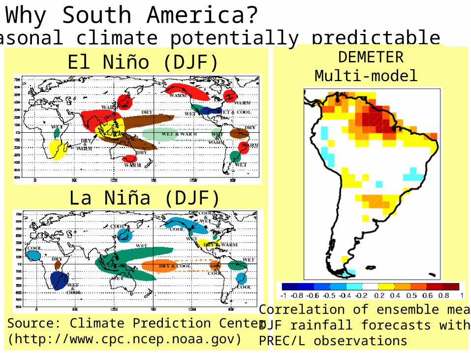
Why South America?

El Niño (DJF)

La Niña (DJF)

Source: Climate Prediction Center (http://www.cpc.ncep.noaa.gov)

Seasonal climate potentially predictableDEMETER

Multi-model

Correlation of ensemble meanDJF rainfall forecasts withPREC/L observations

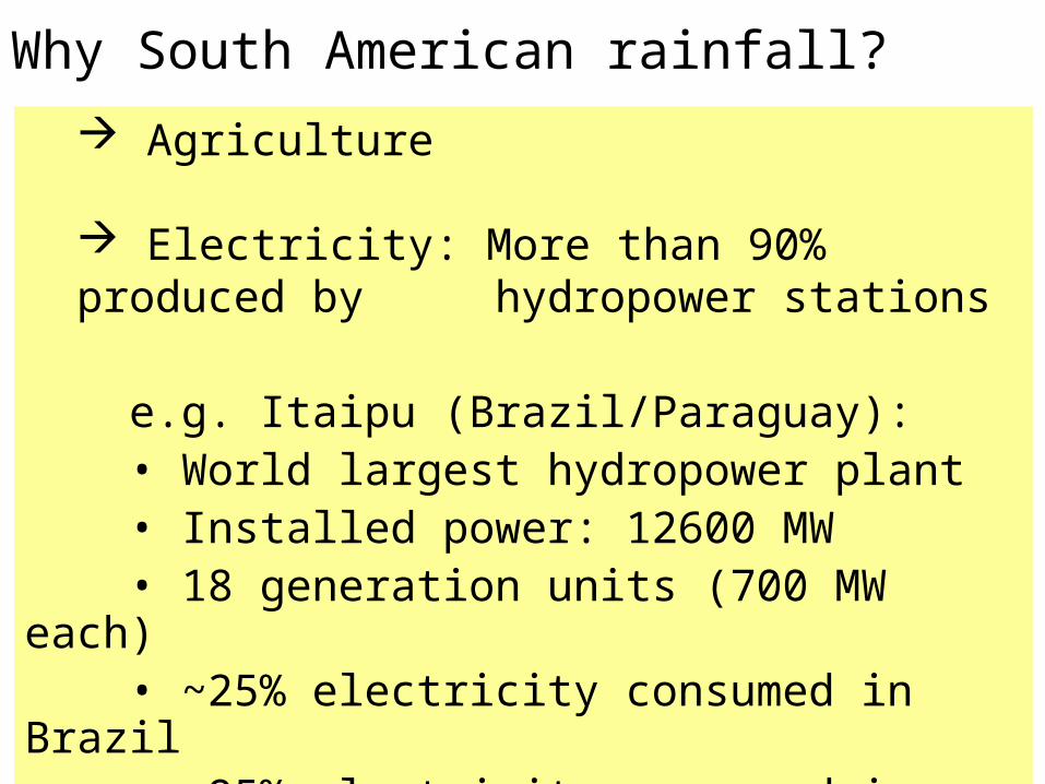
Why South American rainfall?

Agriculture

Electricity: More than 90% produced by hydropower stations

e.g. Itaipu (Brazil/Paraguay):• World largest hydropower plant• Installed power: 12600 MW • 18 generation units (700 MW each)• ~25% electricity consumed in Brazil• ~95% electricity consumed in Paraguay

Itaipu

Example 3: S. American rainfall anomaly composites

Obs Multi-modelForecastAssimilation

(mm/day)

DEMETER: 3 coupled models

(ECMWF, CNRM, UKMO)

1-month lead

Start: Nov DJF

ENSO composites: 1959-2001

• 16 El Nino years

• 13 La Nina years

ACC=0.51

ACC=0.28

ACC=0.97

ACC=0.82

ACC=1.00

ACC=1.00

ACC=Anomaly Correlation CoefficientSpatial correlation of map with obs map

DJF rainfall anomalies for 1975/76 and 1982/83Obs Multi-model Forecast

Assimilation

(mm/day)

ACC=-0.09

ACC=0.32

ACC=0.59

ACC=0.56

La Nina1975/76

El Nino1982/83

DJF rainfall anomalies for 1991/92 and 1998/99Obs Multi-model Forecast

Assimilation

(mm/day)

ACC=0.04

ACC=0.08

ACC=0.32

ACC=0.38

Brier Skill Score for S. American rainfall

Forecast assimilation improves the Brier Skill Score (BSS) in the tropics

limcBS

BS1BSS

)0YPr(p tt

Reliability component of the BSS

Forecast assimilation improves reliability over many regions

limc

reliabreliab BS

BSBSS

Resolution component of the BSS

Forecast assimilation improves resolution in the tropics

limc

resolresol BS

BSBSS

oY | Z ~ N(M[Z Z ],T)1

YZ ZZM S S

oMZ Y MZ 1 T

YY YZ ZZ YZT S S S S

Empirical model for South American rainfall

Y : n q

Z : n p

T : q q

M : q p

Matrices

Z: ASO SSTY: DJF rainfall

Empirical Multi-model Integrated

Correlation maps: DJF rainfall anomalies

Comparable level of determinist skillBetter skill in tropical and southeastern South America

Mean Anomaly Correlation Coefficient

Most skill in ENSO years and forecast assimilation can improve skill

Multi-modelIntegrated

Empirical

limcBS

BS1BSS )0YPr(p tt

ENS

Forecast assimilation improved Brier Skill Score (BSS) in the tropics

Brier Skill Score for S. American rainfall Empirical Multi-model Integrated

limc

reliabreliab BS

BSBSS

Forecast assimilation improved reliability in many regions

Reliability component of the BSS Empirical Multi-model Integrated

limc

resolresol BS

BSBSS

Forecast assimilation improved resolution in the tropics

Resolution component of the BSSEmpirical Multi-model Integrated

Example 4: regional rainfall downscaling

Multi-model ensemble

3 DEMETER coupled models

ECMWF, CNRM, UKMO

3-month lead

Start: Aug NDJ

Period: 1959-2001

Forecast Correlation Brier Score

Multi-model 0.57 0.22

FA 0.74 0.17

South box: NDJ rainfall anomaly Multi-model

Forecast assimilation

Forecast assimilation improves skill substantially

- - - Observation Forecast

Forecast

Forecast Correlation Brier Score

Multi-model 0.62 0.21

FA 0.63 0.18

- - - Observation

Forecast assimilation improved skill marginally

North box: NDJ rainfall anomaly Multi-model

Forecast assimilation

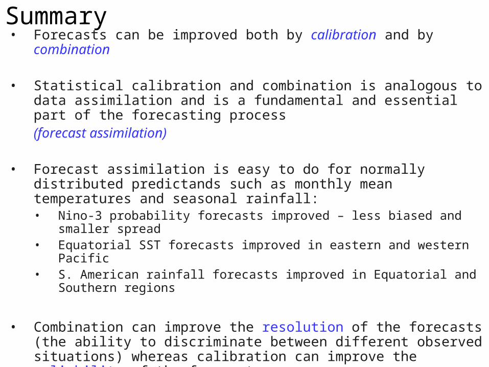
• Forecasts can be improved both by calibration and by combination

• Statistical calibration and combination is analogous to data assimilation and is a fundamental and essential part of the forecasting process (forecast assimilation)

• Forecast assimilation is easy to do for normally distributed predictands such as monthly mean temperatures and seasonal rainfall:• Nino-3 probability forecasts improved – less biased and smaller spread• Equatorial SST forecasts improved in eastern and western Pacific• S. American rainfall forecasts improved in Equatorial and Southern regions

• Combination can improve the resolution of the forecasts (the ability to discriminate between different observed situations) whereas calibration can improve the reliability of the forecasts

• First steps towards an integrated seasonal forecasting system for South America including both empirical and coupled model predictions

• EUROBRISA project will implement this system at CPTEC - Brazil

Summary

The EUROBRISA ProjectLead Investigator: Caio A.S. Coelho

Key Idea: To improve seasonal forecasts in S. America:a region where there is seasonal forecast skill and useful value.

Aims• Strengthen collaboration and promote exchange of expertise and information between European and S. American seasonal forecasters

• Produce improved well-calibrated real-time probabilistic seasonal forecasts for South America

• Develop real-time forecast products for non-profitable governmental use (e.g. reservoir management, hydropower production, and agriculture)

EUROBRISA was approved by ECMWF council in June 2005

http://www.met.rdg.ac.uk/~swr01cac/EUROBRISA

Institutions Country Partners

CPTEC Brazil Coelho, Cavalcanti, Silva Dias, Pezzi

ECMWF EU Anderson, Balmaseda, Doblas-Reyes, Stockdale

INMET Brazil Moura, Silveira

Met Office UK Graham, Davey, Colman

Météo France France Déqué

SIMEPAR Brazil Guetter

Uni. of Reading UK Stephenson

Uni. of Sao Paulo Brazil Ambrizzi, Silva Dias

CIIFEN Ecuador Camacho, Santos

Reliability diagram (Multi-model)

(pi)

(oi)

o

Direct and inverse regression

y

Regression of obs on forecasts Regression of forecasts on obs

More natural to model uncertainty in forecasts for a given observation(ensemble spread of dots) than to model uncertainty in observationsfor a given ensemble forecast. so we model the likelihood on right ratherthan the more common forecast calibration (MOS) approach on the left.

),X28.168.6(N~X|Y 2X|Y ),Y73.065.6(N~Y|X 2

Y|X

Reliability diagram (FA 58-01)

o

(pi)

(oi)

Moment measure of skewness

n

1i

3

y

i1 s

yy

n

1b

Measure of asymmetry of the distribution