Global J. Environ. Sci. Manage. 7(3): 457-472, Summer 2021

*Corresponding Author:Email: chandramani106@gmail.comPhone: + 8794885778Fax: 0385-2413031

Global Journal of Environmental Science and Management (GJESM)

Homepage: https://www.gjesm.net/

CASE STUDY

Linking the past, present and future scenarios of soil erosion modeling in a river basin

C. Loukrakpam*, B. Oinam

Department of Civil Engineering, National Institute of Technology Manipur, Langol Road, Lamphelpat, Imphal, Manipur, India

BACKGROUND AND OBJECTIVES: Soil erosion is considered one of the major indicators of soil degradation in our environment. Extensive soil erosion process leads to erosion of nutrients in the topsoil and decreases in fertility and hence productivity. Moreover, creeping erosion leads to landslides in the hilly regions of the study area that affects the socio-economics of the inhabitants. The current study focuses on the estimation of soil erosion rate for the year 2011 to 2019 and projection for the years 2021, 2023 and 2025.METHODS: In this study, the Revised Universal Soil Loss Equation is used for estimation of soil erosion in the study area for the year 2011 to 2019. Using Artificial Neural Network-based Cellular Automata simulation, the Land Use Land Cover is projected for the future years 2021, 2023 and 2025. Using the projected layer as one of the spatial variables and applying the same model, Soil Erosion based on Revised Universal soil loss equation is projected for a corresponding years. FINDINGS: For both cases of projection, simulated layers of 2019 (land use land cover and soil erosion) are correlated with the estimated layer of 2019 using actual variables and validated. The agreement and accuracy of the model used in the case land use are 0.92 and 96.21% for the year 2019. The coefficient of determination of the model for both simulations is also observed to be 0.875 and 0.838. The simulated future soil erosion rate ranges from minimum of 0 t/ha/y to maximum of 524.271 t/ha/y, 1160.212 t/ha/y and 783.135 t/ha/y in the year 2021, 2023 and 2025, respectively.CONCLUSION: The study has emphasized the use of artificial neural network-based Cellular automata model for simulation of land use and land cover and subsequently estimation of soil erosion rate. With the simulation of future soil erosion rate, the study describes the trend in the erosion rate from past to future, passing through present scenario. With the scarcity of data, the methodology is found to be accurate and reliable for the region under study.

©2021 GJESM. All rights reserved.

ARTICLE INFO

Article History:Received 28 November 2020 Revised 02 March 2021 Accepted 13 March 2021

Keywords:Artificial neural network (ANN)Cellular automata (CA)RUSLESoil erosion

ABSTRAC T

DOI: 10.22034/gjesm.2021.03.09

NUMBER OF REFERENCES

33NUMBER OF FIGURES

10NUMBER OF TABLES

6

Note: Discussion period for this manuscript open until October 1, 2021 on GJESM website at the “Show Article.

458

C. Loukrakpam, B. Oinam

INTRODUCTIONVarious naturally occurring resources are

available around us, but soil and water resources are considered to be indicative of all. An increase in population in due course of time associates with increasing anthropogenic pressures to these resources. Checking these pressures and opting for practices that focus on the optimized use of resources with minimum stress on the environment can only lead to sustainable development, which is indeed needed in the time ahead (Renard et al., 1997). Land degradation is the state due to which the trait of soil is decreased both in physical composition and chemical combination, as an aftermath of a certain phenomenon due to certain factor. Soil erosion is the most significant environmental problem which leads to land degradation. It is defined as the damage of topsoil by natural agents (Gallaher and Hawf, 1997). The loose soil carried away by the agents during the soil erosion process transports anthropogenic toxic substance into drainage systems, which in turns causes other environmental pollutions (Sandra et al., 2015). Exposure of the topsoil during rainfall; then detachment of loose particles and deposition of the particles is the stages involved in the soil erosion phenomena. These processes are associated directly with the changing land use and land cover pattern of the region (McCool et al., 1978). Thus, soil erosion can be related to changing LULC patterns, changes in topography, soil composition attributed to the area. Manipur lies in the eastern part of the Himalayan range and comprises hilly terrain which covers the majority of the total geographic area, except for the valley in the central portion of the state. Due to its topography and changing LULC pattern and various anthropogenic factors, the state is prone to land degradation. According to the study regarding land degradation, in 2011-2013, 26.96% of the total geographic extent is under degradation. 25.78% of the above-mentioned percentage is due to vegetation degradation and 0.36% is due to soil erosion (SAC, ISRO, 2016). The geospatial technique is a widely used technique for studying the environmental phenomenon because of its ability to integrate the various variable parameters and gives the synoptic view of the study area. These tools and techniques can be applied in the computation of the rate of soil erosion, evaluating processes and understanding its underlying parameters about the region (Jahun et

al., 2015). The revised universal soil loss equation (RUSLE), Geographic information system (GIS)-based model is one of the most widely used soil erosion model and is improved model of original soil erosion model developed by Wischmeier and Smith, 1978 (Renard et al., 1997). Models such as USLE had also been used for assessing the soil erosion rate in the river basin of the hilly terrain of North East India (Ghosh, et al., 2013). Physical models such as water erosion prediction project (WEPP), unit stream power- based erosion deposition (USPED) and European soil erosion model (EUROSEM) which requires complex input variables is not applied in this study due to the scarcity of data (Mitas and Mitasova, 2001; Smets, et al., 2011; Ahmadi, et al., 2020). The use of slope length factor in RUSLE enables to estimate the overland flow of the agricultural area. The model has advantages of limited data requirement, which is important for research in data-scarce regions like the study area and simplicity in computation. Hence, RUSLE is used for the assessment of soil rate in this study. NBSS & LUP, CSWCR&TI and Department of Horticulture and Soil Conservation, Government of Manipur jointly undertook the task for preparation of soil resource map and conducted soil erosion assessment for the state of Manipur, India, using USLE. The assessment detail the soil loss in the state, which also encompassed the study area for the year 1996 and 2006 (Sen et al., 1996; Sen et al., 2006 ). In this study, estimation of soil erosion rate in Manipur river basin for the past 9 years (2011- 2019) and predicting the soil erosion rate of 2021, 2023 and 2025 has been the main emphasis. ANN-based CA model has been successfully implemented for predicting the future changes in land use land cover pattern (El-Tantawi, et al., 2019; Gharaibeh, et al., 2020; Yang, et al., 2016). For predicting the future soil erosion rate, a Projected LULC is required, which is done using MOLUSCE simulation. MOLUSCE, a Quantum GIS platform-based tool enables the convenient assessment for land-use change modelling. The model employed artificial neural network (ANN) based cellular automata model for simulation (Rahman et al., 2017; Saputra and Lee, 2019). The neural network, which is an adaptive system, is used in the study to estimate the vegetative index of future years. Time series vegetative index data are train and test in the neural network environment (Abujayyab and Karas, 2019). Projected vegetative index named Normalized

459

Global J. Environ. Sci. Manage., 7(3): 457-472, Summer 2021

Difference Vegetative Index is also employed as one of the inputs in the assessment. The application of the machine learning techniques for the projection of future scenarios; the use of simulated data and integration for projecting another future scenario is the main focus in this study. The primary aim of this study is a) Estimation of soil erosion rate for years (2011-2019), Spatio-temporally; b) prediction of projection of the rate of soil erosion for the year 2021, 2023 and 2025.

MATERIALS AND METHODSStudy area

The Loktak catchment and Chakpi river watershed and Manipur River watershed constitute the Manipur River Basin. Areal extent of basin is about 6872 sq.km, which is almost 31% of the expanse of Manipur state (Fig. 1). It comprises nine watersheds namely Imphal River Watershed, Upper Iril River Watershed, Lower Iril River Watershed, Thoubal River Watershed, Heirok River Watershed, Khuga River Watershed, Loktak Watershed, Chakpi River watershed and Manipur River Watershed. Soil composition of the basin differs along with the topography. Hill soil comprises of red soil due to oxidisation and a usually weathered at

the foothills, and valley soil ranges from silt loam to clayey texture. The average precipitation of the basin ranges between 1200 to 1350 mm and temperature between 19°C to 21°C. The elevation of the basin is 720 to 800 m above mean sea level in the valley and rises up to 2684m in the hilly region and average slope of 15 degree. As the basin encompassed almost of all the valley region of the state, the population of the inhabitant is about 90% of the total population of the state of Manipur. Most of the agricultural practices are found in the valley region of the study area and also in some regions of hilly region. Tropical deciduous types of forest are found in the study area. (Trisal and Manihar, 2004).

Extensive percent of total built-ups and agricultural lands are situated in the valley region of the basin. Dynamic nature of built-ups and agricultural land affects the land cover, which is due to increase in inhabitant population which in turn makes land cover susceptible to soil erosion.

Data acquisition and methodologyFor input as spatial variables, drainage distance

raster and elevation raster is derived from DEM; and road distance raster is developed using the

Fig. 1: Geographical location of the study area, Manipur River Basin, Manipur, India

Fig. 1: Geographical location of the study area, Manipur River Basin, Manipur, India

460

Soil erosion scenarios in a river basin

road network layer procured from north east space application centre, India. In both cases i.e. past and future soil erosion assessment, soil layers and topographic features are considered to be constant.

RUSLE soil erosion estimationRUSLE is based on physical variables such slope

length factor; soil erodibility factor; supporting conservation practices factor; crop management factor and rainfall erosivity (Sehgal and Abrol, 1994). RUSLE was originally designed for use in plot size or field size study area but due to its applicability, it is now often used for various scales using Eq. 1 (Panos et al., 2014).

A R C P K LS= × × × × (1)

Where, A is the rate of soil erosion in ton/ha.year; R is Rainfall Erosivity factor in MJ.mm/ha/ h/y; K is Soil Erodibility factor in ton.ha.h/ha.MJ.mm; LS is Slope Length factor; P is Practice Management Factor and C is Crop management Factor.

Variables used as input for estimation, in the model have varying spatial resolution. The entire inputs variables layer has been resampled to 30m spatial resolution to have spatial homogeneity, and thus the model is processed.

R – Factor Intensity of the contact of rainfall drops with

the ground is signified by the Rainfall Erosivity. Raindrop has compelling effect on soil erosion rate and the surface run-off and is signifies by R-Factor (Wischmeier and Smith, 1978). The gridded precipitation data are acquired from Climate hazards group infrareds precipitation with station data portal for past years and from NASA NCCS downscaled

precipitation for future years. Both the acquired datasets have different spatial resolutions (Table 1) which are resample to 30m resolution for estimation of the rainfall erosivity factor. Daily precipitations data is acquire in both the case and are total monthly and eventually yearly manner for implementation in the equation. Eq. 2 describes the Rainfall erosivity equation used in this study using (Arnoldus H.M.J., 1980).

12

11.735*1010

Pi(1.5log ( ) 0.08188)P10R

−=∑ (2)

Where, R is Rainfall Erosivity factor in MJ.mm/ha/ h/y; Pi is Monthly Precipitation (mm); P is Annual Precipitation.

K – FactorImpediment of loose soil against transportation

and detachment based on the physical texture and carbon content is estimated as K-Factor. The factor is express in (ton/ha/h)/ (ha/MJ/mm) (Wischmeier et al., 1971). The soil of the study area is characterized as deep, rich in organic carbon content, slightly acidic and rich in nitrogen, potassium and low in phosphorous (Sarkar et al., 2002). In this study, the soil physical properties are considered to be constant and remain unchanged, i.e. for past years and for prediction same soil layers are used for the generation of soil erodibility layer. The gridded soil layer dataset namely Sand fraction percent, Silt fraction percent, Clay fraction percent and Organic carbon content is acquired from World Soil Information data portal. The acquired data is process and resample and used for estimation of soil erodibility of past years soil erosion and predicting future soil erosion rate. K- Factor is estimated using the equation, Eq. 3 (Sharpley and

Table 1: Input data and sources

Satellite/sensor/source Description Resolution Landsat-7 ETM+ C1 level1 Year: 2011 - 2013 30m Landsat 8 OLI/TIRS C1 level 1 Year: 2014 - 2019 30m CHIRPS* Precipitation data: year 2011-2019 5.55km NEX- GDDP dataset* Precipitation data: Year 2021, 2023 and 2025 ~ 25km MODIS (MOD13Q1)* NDVI data: year 2011-2019 250 m World soil information data portal* Soil physical raster data 250 m SRTM DEM dataset, drainage distance layer 30 m Road network, NESAC, India Road distance raster layer 30 m

* Dataset spatial resolution resample to 30m

Table 1: Input data and sources

461

Global J. Environ. Sci. Manage., 7(3): 457-472, Summer 2021

Williams, 1990)

(3)

([0.2 0.3 exp{ 0.02561( )}] ( )

1000.25 .{1 }

. exp(3.75 2.95 . )

0.7 (1 )100{1 } 0.1317)

(1 ) exp( 5.51 22.9 (1 )100 100

K SandSilt Silt

Clay Siltorg C

org C org CSand

Sand Sand

= + × − × ×−

×+×

× −+ − ×

× −× − ×

− + − + × −

Where, K is soil erodibility factor; sand is sand fraction percent; silt is silt fraction percent; clay is clay fraction percent and org. c is organic carbon content.

LS – Factor Topographical factor indicating the distance of the

origin point of erosion to the deposition point, as a result of the slope is determined by the slope-length factor. Higher overland flows velocities are attributed to and correspondingly higher erosion (Renard et al., 1997; Wischmeier and Smith, 1978). In this study, the physical-based slope length factor is calculated using the satellite-based elevation model data, which is used in RUSLE (Both past years and future years), using Eq. 4 (Moore and Burch, 1986).

sin( ) ( )22.13 0.0896

A m nLS θ= ×

(4)

Where LS is the slope length factor; A is Catchment Area; θ is slope angle in percent (%)

m = 0.4 and n = 1.3

C - FactorInfluences of vegetation coverage in the soil

erosion rate estimation are significant. C - Factor is the variable which is defined as the correlation between the soil erosions from cropped land with the defined condition and corresponding erosion till cleaned, fallow continuously (Wischmeier and Smith, 1978). Vegetation index such as NDVI has been employed for the estimation of C- factor, but the equation used for calculation differs according to the geographic region under study. The equation used for assessment in the mid latitudinal region (Van der Knijff, et al., 2000) is found to be unsuitable for tropical region and hence different equation is used for this region, using Eq. 5

and 6 (Durigon et al., 2014).

REDNIRREDNIR

NDVI

)2

1NDVI(C

+−

=

+−=

(5)

REDNIRREDNIR

NDVI

)2

1NDVI(C

+−

=

+−=

(6)

Where, C is Crop Management Factor Management; NDVI is Normalized Difference Vegetation Index; NIR is Near Infra-Red band; RED is the Red Band of imagery used.

MODIS NDVI dataset, which is of 250 m spatial resolution, is used in this study. The composite NDVI layer for each year is generated and extracted for the study area region and is resampled to 30m for estimation of C – Factor using Eq. 5.

P – FactorVariable used in RUSLE, which is a correlation

between the soil erosion with a specific support practice and the corresponding erosion with upslope and downslope cultivation. Relation between land use variable and slope factor is developed so that the impact on runoff, drainage and velocity resulting from control practice are considered. The assigned value of P-factor to specific land use class slope is given Table 2. (Wischmeier and Smith, 1978). P – Factor layer is generated by combining the LULC layer for each year and slope layer generated from DEM. LULC layer for each years are classified into ‘Agriculture’ class and ‘Other Land Use’ class and slope layer is reclassified into six classes as shown in Table 2.

MOLUSCEThe model performs the transition potential

modelling based on Markovian approach and uses four different models namely Logistic Regression (LR); Artificial Neural Network; Weight of Evidence

Table 2: Assigned P-factor value for different land use and slopes

P- factor Land use Slope (%) 0.100 Agriculture 0 – 5 0.120 5 – 10 0.140 10 – 20 0.190 20 – 30 0.250 30 – 50 0.330 50 – 100 1.000 Other land use All

Table 2: Assigned P-factor value for different land use and slopes

462

C. Loukrakpam, B. Oinam

(WoE) and Multi-Criteria Evaluation (MCE) for training simulation model (NEXTGIS, 2017). Logistic regression analysis is a statistical approach of training the sample data to develop Relationship between dependent variable and sets of independent variable. Finally, the independent variable which has the best correlation will be selected for prediction. Artificial neural network is an adaptive system which develops the relation between variables so that it could be trained to recognize pattern, classify data and predict the data. Sigmoidal function is used to train the sample data. Weight of evidence training model was initially develop to train only binary model, but was later modified so that it could train continuous data. In this module, the continuous data are categorized into classes (maximum of 100 classes) and weights are estimated to predict the data. Multi criteria evaluation training model is based on Saaty’s hierarchal analysis. It is a systematic approach to make decision for complex problems (GIS Lab, 2018). In this study, Cellular Automata - ANN approach is used for predicting future LULC and soil erosion rate for the area under study. LULC layers (Years 2011-2019) are generated using Maximum Likelihood Classification technique employing Landsat multispectral imageries as inputs. LULC of the year 2019, 2017, 2015 and 2013 is used as inputs in the MOLUSCE model to generate the Projected LULC of 2021, 2023 and 2025. Road distance raster layer, Drainage distance layer and elevation are employed as the spatial variable (Driving Factor) for the ANN Transition potential modelling. Pearson’s Correlation method is used in the model tool for calculating the correlation among the spatial variables or driving factors, which are in turn used in ANN potential modelling. Projected future LULC is generated using CA Simulation. Road distance raster layer is generated using the road network file and drainage distance and Elevation are obtained from SRTM-DEM. To validate the model and to assess the degree of agreement and accuracy, LULC of the year 2019 is simulated using LULC of the 2017 and 2018. The simulated LULC of 2019 is validated using the actual LULC of 2019, which is generated using Landsat Imageries as mentioned above. MOLUSCE model tool is widely used for projection of the future LULC. However, for this study, the tool is used for simulation and projection of soil erosion class also. As the input layers should be qualitative raster, the quantitative soil erosion rate raster obtained from

RUSLE is classified to qualitative form and is used as inputs. Soil erosion datasets of 2019, 2017, 2015 and 2013 are used for projecting the future soil erosion of years 2021, 2023 and 2025. In the case of Soil Erosion simulation, Drainage distance, Elevation, LULC and precipitation for the year to be simulated are used spatial variable or driving factor. Simulated LULCs of the future years are input as spatial variables for each case and future projected precipitation is acquired from NASA Earth Exchange Global Daily Downscaled Projection (NEX – GDDP) precipitation dataset (Thraser et al., 2012). Similar to previous case, Pearson’s Correlation method is used in the model tool for calculating the correlation among the spatial variables or driving factors, which are in turn used in ANN potential modelling and simulation is done by CA approach. As in the case of LULC future dataset simulation, validation for the agreement and accuracy of the model is done by simulating the soil erosion dataset of the year 2019 using the soil erosion dataset of 2017 and 2018 and follows by validation using the actual soil erosion dataset of the year 2019.

RESULTS AND DISCUSSIONSoil erosion rate estimation

The estimated soil erosion rate is classified into five soil erosion classes. Classification by NBSS and LUP is adapted for classifying the soil erosion class for this study. According to this adaptation, the classified soil erosion qualitative classifications are ‘No Erosion’ (<5 t/ha/y); ‘Slight Erosion’ (5 to 10 t/ha/y); ‘Moderate Erosion’ (10 to 20 t/ha/y); ‘High Erosion’ (20 to 40 t/ha/y) and ‘Intense Erosion’ (> 40 t/ha/y) (Table 3). According to the study adapted above, soil erosion less than 5 t/ha/y shows no effect on the effectiveness of the conservative structure. Thus the tolerable soil erosion limit of the study area is taken to be soil erosion rate less than 5 t/ha/y (Sen et al., 2006). The corresponding area in square km.

Table 3: Soil erosion rate classification limit (based on national bureau of soil survey and land use planning)

Class Range (t/ha/y) No Erosion < 5 Slight Erosion 5 - 10 Moderate Erosion 10 - 20 High Erosion 20 - 40 Intense Erosion > 40

Table 3: Soil erosion rate classification limit (based on national bureau of soil survey and land use planning)

463

Global J. Environ. Sci. Manage., 7(3): 457-472, Summer 2021

for the Soil Erosion class for the years 2011 to 2019 is shown in Fig. 2. Even though there is variation in the area under ‘No Erosion’ class, an increasing trend is observed overall in this class from the year 2011 to 2019. 2013 has lowest percentage with 39.36% and 2018 and 2019 have the highest with 48.69% and 48.57% respectively. ‘Slight Erosion’ in the study area is observed to follow the increasing trend during the period of study. With percentage 5.10% in the 2011 increases up to 14.53% in 2018 and 13.27% in 2019. Gradual increment with variation is observed in the ‘Moderate Erosion’ class. Except for 2013, where the percentage declines to 12.40%, remaining years shows the gradual rise in percentage from 22.81% in 2011 to 29.92% in 2017. In case of ‘High Erosion’ class, a positive response is observed throughout the period under study. The percentage of total area under this class has been gradually reducing since 18.16% in 2011 to 6.30% and 7.13% in 2018 and 2019, except for slight increment up to 18.64% in 2013. ‘Intense Erosion’ class also indicates positivity, as there is decline in the total percentage of area coverage in this class over the year. From 12.96% in 2011 to 3.32% and 3.80% in 2018 and 2019 respectively, except for an abrupt rise to 25.18% in 2013.

The range of soil erosion rate for the year 2011 to 2019 is depicted in maps in Fig. 3. Quite a variation is observed in the maximum soil erosion rate from the year 2011 to 2019. An increasing trend is followed from the year 2011 to 2015 with maximum soil

erosion rate 776.63 t/ha/y to 1253.7 t/ha/y and then decreasing trend follows to 2019 estimating the maximum soil erosion rate of 266.45 t/ha/y (Table. 4).

Future LULC projection using MOLUSCEUsing MOLUSCE model tool, LULC of the future

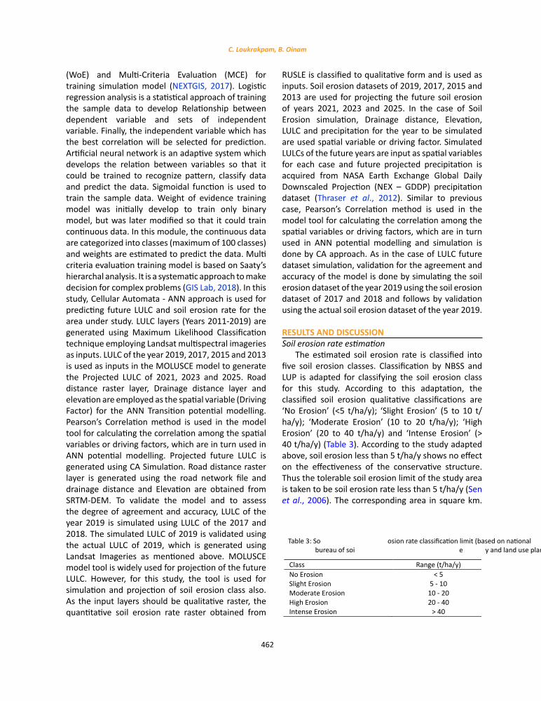
year 2021, 2023 and 2025 of the study area has been projected in this study (Fig. 4). In the projected future LULC, variations in the spatial extent of the land use class is observed as result. Area under ‘Vegetation’ class shows decrease in area from the year 2021 to 2023 and then grows in the year 2025. Spatial extent of classes ‘Agriculture’;’ Water Bodies’ and ‘Barren’ shows similar trends of change in area. Area coverage increases from 2021 to 2023 and decreases in the year 2025. ‘Built Up’ class shows growth in the most unique pattern. Extent of area coverage expanse over the time from 2021 to 2025 and is shown in Fig. 5.

In this study, ANN based transition potential modelling is performed and sample data are train. Then, the trained data are used for CA simulation and simulated layer is generated. For validation of the output simulated layer, accuracy assessment, kappa statistics is done and overall accuracy of the model is found to be 96.21% for 2019 simulation. Also, agreement of the model expressed in terms of Kappa Coefficient is observe as 0.92 which is almost perfect model (Landis and Koch, 1977). Regression analysis is perform between area of each classes from actual LULC 2019 and projected LULC 2019 so as

Fig. 2: Area under different soil erosion class in km2 (2011-2019)

0

500

1000

1500

2000

2500

3000

3500

No Erosion Slight Erosion ModerateErosion

High Erosion Intense Erosion

Area

in sq

.km

Soil Erosion Class

Soil Erosion Class 2011-2019

2011 20122013 20142015 20162017 20182019

Fig. 2: Area under different soil erosion class in km2 (2011-2019)

464

Soil erosion scenarios in a river basin

Fig. 3: Soil erosion maps (2011-2019)

Fig. 3: Soil erosion maps (2011-2019)

465

Global J. Environ. Sci. Manage., 7(3): 457-472, Summer 2021

to determine the proportion of variance dependent variable i.e. projected LULC 2019. The co-efficient of determination, R2 of the regression is found to be 0.875 which shows the high accuracy of the model.

Future soil erosion projection using MOLUSCEThe projected future soil erosion depicts

the future trend in quite a positive nature when comparison is done with the soil erosion layer of

Fig. 4: Projected LULC map of 2021, 2023 and 2025

Fig. 4: Projected LULC map of 2021, 2023 and 2025

Fig. 5: Area under different LULC classes of 2021, 2023 and 2025

0.00

1000.00

2000.00

3000.00

4000.00

Vegetation Agriculture Built Up Water Bodies Barren

Area

in sq

.km

Land Use Class

Projected LULC (2021, 2023, 2025)

2021

2023

2025

Fig. 5: Area under different LULC classes of 2021, 2023 and 2025

Table 4: Area of the land use classes (areas in km2)

Class/Value LULC 2019 Projected LULC 2019 Residual Vegetation 3271.954 3394.049 96.403 Agriculture 904.691 930.366 97.240 Built Up 531.307 471.686 112.640 Water Bodies 236.993 249.148 95.122 Barren 1787.161 1686.856 105.946

Table 4: Area of the land use classes (areas in km2)

466

C. Loukrakpam, B. Oinam

Fig. 6: (a) LULC 2019 vs projected LULC 2019 map; (b) LULC 2019 vs projected LULC 2019 (Areas in km2)

Fig. 6: (a) LULC 2019 vs projected LULC 2019 map; (b) LULC 2019 vs projected LULC 2019 (Areas in km2)

Fig. 7: Soil erosion classes map for the year 2021, 2023 and 2025

Fig. 7: Soil erosion classes map for the year 2021, 2023 and 2025

467

Global J. Environ. Sci. Manage., 7(3): 457-472, Summer 2021

2019 (Fig. 7). Variation in the soil erosion rate is observed from the estimated layers. Maximum soil erosion rate increases abruptly from 52.4.271 t/ha/y in year 2021 to 1160.212 t/ha/y in 2023. Again, the maximum ranges down to 783.135 t/ha/y in 2025 (Fig. 7). Resultant soil erosion rate is classified in five qualitative class based on the classification shown in

Table 3. As depicted in graphical format in Fig. 8, the soil erosion classes namely ‘Moderate Erosion’; ‘High Erosion’ and ‘Intense Erosion’ shows the decreased in area coverage over the time and ‘No Erosion’ and ‘Slight Erosion’ class shows the increase in area as the time lapses. In case of ‘No Erosion’ class, there increase in area coverage is observed with 6.14%,

Fig. 8: Area under different soil erosion classes for the year 2021, 2023 and 2025 (Areas in km2)

0500

1000150020002500300035004000

No Erosion Slight Erosion ModerateErosion

High Erosion Intense Erosion

Area

in sq

.km

.

Soil Erosion Class

RUSLE Soil Erosion(2021, 2023 & 2025)

2021

2023

2025

Fig. 8: Area under different soil erosion classes for the year 2021, 2023 and 2025 (Areas in km2)

Fig. 9: Soil erosion test site within the basin

Fig. 9: Soil erosion test site within the basin

468

C. Loukrakpam, B. Oinam

6.70% and 8.26% of total area in 2021, 2023 and 2025 respectively. Areas under ‘Slight Erosion’ class decreases 1.49% to 0.22% in 2021, 2023 and then, increases to 1.07% in 2025. Highest rate of decreases in the area is observed in the ‘Moderate Erosion’ class. The area declines by 2.49% in 2021, 4.37% in 2023 and 4.80% in 2025. The area under ‘High Erosion’ class reduces with 1.30% in 2021, 1.07% and 1.35% in 2023 and 2025 respectively. ‘Intense Erosion’ class also shows declining in the area, which is a positive indication. 0.86% is decrease in 2021, 1.05% in 2023 and 1.04% in 2025 is the percentage of area decrease under the above mention class.

Validation of future soil erosion rate modelFor the validation of the model, a plot scale

catchment is considered within the study area as test site. The total area of the test site is 135809.30 sq.m., which is a plantation site. For estimating the

soil erosion rate of the test site, observed data such as topographic survey is conducted using total station every month for the year 2019, NDVI is measured using the NDVI meter and soil samples are taken. Elevation profile of the test site is obtained and thus slope length factor is estimated. C- Factor is estimated using the NDVI data and P-factor is estimated using the land use and slope layer which is generated using the elevation layer. K- Factor is estimated by testing the soil samples and finally R- factor is estimated using the precipitation data obtained from the automatic weather station installed nearby the test site. Thus, soil erosion rate of the test site is estimated for the year 2019.

Validation of the model is performed by using the observed soil erosion rate layer of the year 2019 (observed 2019). For model validation, using the same model-simulated soil erosion rate layer of 2019 (simulated 2019) is also generated. Random 155

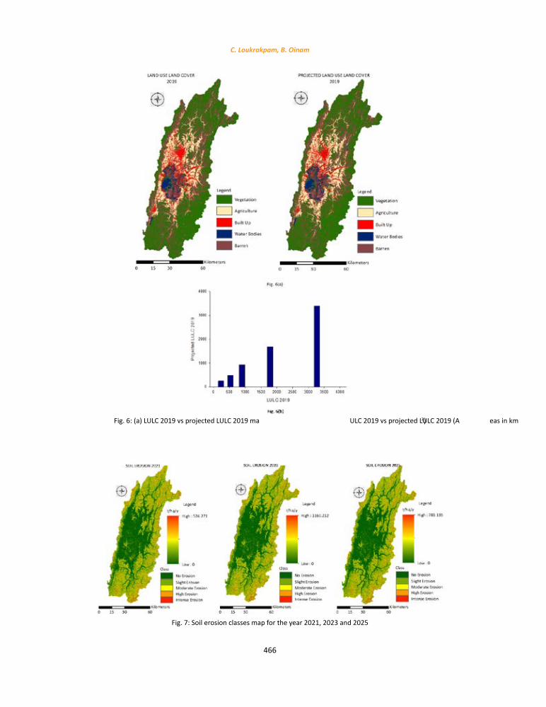
Fig. 10: Observed soil erosion rate Vs simulated soil erosion rate

0

5

10

15

20

25

0 5 10 15 20 25

Soil ErosionObserved Vs Simulated

Sim

ulat

edSo

il Er

osio

n Ra

tet/

ha/y

Observed Soil Erosion Ratet/ha/y

Fig. 10: Observed soil erosion rate Vs simulated soil erosion rate

Table 5: Area under each class for soil erosion 2019 and projected soil erosion 2019 (areas in km2)

Class Observed Simulated Residual No Erosion 0.088 0.100 0.012

Slight Erosion 0.044 0.036 -0.008

Moderate Erosion 0.007 0.004 -0.004

Table 5: Area under each class for soil erosion 2019 and projected soil erosion 2019 (areas in km2)

469

Global J. Environ. Sci. Manage., 7(3): 457-472, Summer 2021

sample points are selected within the test site with ground coordinates. Using geospatial techniques, the soil erosion rate value corresponding to each sample point are extracted from the observed soil erosion layer and also from the simulated soil erosion layer of 2019. As the attributes of the point have soil erosion rate value of both observed and simulated layer, the attribute is exported as the table. The soil erosion rate of the two layers ranges from 0 to 14.10 t/ha/y for the observed data and 0 to 12.49 t/ha/y for simulated data. Using the data from the table, regression analysis is performed between observed and simulated soil erosion rate, to determine the variance of simulated data (Fig. 10). The coefficient of determination value, R2 is found to be 0.838, which shows more than 80% of the simulated data can be explained by the observed data. Apart from few outliers observed at some sampling points, the observed data and simulated data are highly correlated. With this percentage of the coefficient of determination quantitatively, the model shows a high percentage of agreement.

For qualitatively validating the model, the observed and simulated soil erosion layers are classified and 3 class is obtained as per maximum soil erosion rate (Table 5). As in case of LULC, which represents qualitative values, regression analysis is performed considering simulated data as dependent variable and observed data as independent variable. The co-efficient of determination, R2 is found to be 0.96, which also shows high percent of agreement. The model is validated quantitatively and qualitatively with high percent of agreement.

Over estimation is observed in the ‘No Erosion’ class and under estimation are observed in the ‘Slight Erosion’ and ‘Moderate Erosion’ class. The soil erosion studies conducted earlier in the region were found to be of courser temporal resolution, i.e. time gap between the two studies was 10 years. Even though

the output results from the earlier studies were for the whole state of Manipur, the time gap between the outputs were big and is difficult for trend analysis (Sen et al., 1996; Sen et al., 2006). In this study, the resultant outputs are provided for consecutive years and for the future also, hence trend analysis of the soil erosion in the basin can be analyse with ease. Also there is observation, such as increase in area under ‘No Erosion’ class and decrease rate of soil erosion as the analysis is done from past towards future (Table 6).

CONCLUSION The present study focus on the estimation of

the soil erosion rate over the period of 9 years, and also the prediction of future soil erosion rate. As the estimation of the future soil erosion rate is dependent on the projected LULC, the focus has also been over the prediction of future LULC. With the good agreement of the model is observed for prediction of LULC, the estimation of the future soil erosion rate is performed using the same model. The results of the model shows strong correlation with the observed data used for validation, hence the model can be used for estimation of further future soil erosion rate. The result of the model can be improved by using other model if the region has not face the hindrance of data scarcity.

The ranges of the soil erosion rate has been analyse in this study for 2011 to 2019 and 2021, 2023 and 2025. The trending of the maximum range decreases as the study moves forward the time and in future. Higher rate of erosion is observed the past years due to the activity like jhum cultivation, deforestation, slash and burning practice in the hilly region of the basin. As the year moves towards the recent past, there is decrease in the erosion rate due to the new land use policy, afforestation schemes and conservative measure taken up with initiation

Table 6: Range of soil erosion rate from 2011 to 2025 (t/ha/y)

Year 2011 2012 2013 2014 2015 2016 Range t/ha/y

Minimum 0 0 0 0 0 0 Maximum 776.63 604.00 1203.07 886.32 1253.70 1071.79

Year 2017 2018 2019 2021 2023 2025

Range t/ha/y

Minimum 0 0 0 0 0 0 Maximum 631.10 293.72 266.45 524.27 1160.21 783.14

Table 6: Range of soil erosion rate from 2011 to 2025 (t/ha/y)

470

C. Loukrakpam, B. Oinam

from the policy maker. Conservative structures are also encouraged in the hilly region in the recent past hence positive signs towards the environment are observed. The rate of soil erosion increases from 776.63 t/ha/y in 2011 to 1253.7 t/ha/y in 2015 and then decreases to 233.45 t/ha/y in 2019 due to conservative practices followed by the inhabitants. The projected scenario from the study is possible in the future only if we intervene in the degradation activity in the environment at present time. Intense land degradation problems may be solved and sustainable development can be achieved even in this developing region, by considering the results from this study. The result of this study is focusing on the future simulated data which can be made into better results if the policymakers and stakeholders, and none the less, the inhabitants take up conservative measure against the destruction of environments.

AUTHOR CONTRIBUTIONSC. Loukrakpam performed the literature review,

data processing, analysed and interpretation of the data, prepared the manuscript text and manuscript edition. B. Oinam helped in the conceptualization, review of manuscript and presentation of the manuscript.

ACKNOWLEDGMENTSThe authors gratefully acknowledge United States

Geological Survey (USGS), ISRIC, CHIRPS for providing the dataset through the respective archives and North East Space Application Centre (NESAC), India for the datasets used in this study. The authors also express the gratitude for the research conducted, toward Science and Engineering Research Board (SERB) project [YSS/2014/000917], University Grant Commission, Government of India and National Institute of Technology Manipur.

CONFLICT OF INTERESTThe authors declare no potential conflict of

interest regarding the publication of this work. In addition, ethical issues including plagiarism, informed consent, misconduct, data fabrication and, or falsification, double publication and, or submission, and redundancy have been completely witnessed by the authors.

ABBREVIATIONS% PercentageA Rate of soil erosionANN Artificial neural networkC Crop ManagementCA Cellular automata

CHIRPS Climate Hazards Group InfraRed Precipitation with Station

DEM Digital Elevation ModelEq EquationEUROSEM European soil erosion modelexp Exponenth hourha hectare

ISRIC International Soil Reference and Information Centre

K Soil Erodibiltylog LogarithmLR Logistic regressionLS Slope lengthLULC Land Use Land CoverMCE Multi-criteria evaluationMJ Mega Joulemm millimeter

MODIS Moderate resolution imaging spectroradiometer

MOLUSCE Modules for land use change simulations

NASA-NCCSNational Auronautics and Space Administration – NASA Centre for Climate Change Simulation

NBBS & LUP National Bureau of Soil Survey and Land Use Planning

NDVI Normalized difference vegetation index

NESAC North Eastern Space Application Centre

NEX-GDDP NASA Earth Exchange Global Daily Downscaled Projection

NIR Near Infra redP Annual precipitationP Practice management factorPi Monthly precipitationR Rainfall erosivityR2 Coefficient of determinationRUSLE Revised universal soil loss equationSRTM Shuttle radar topographic mission

471

Global J. Environ. Sci. Manage., 7(3): 457-472, Summer 2021

USGS United state geological surveyUSLE Universal Soil Loss Equation

USPED Unit stream power-based erosion deposition

WEPP Water erosion prediction projectWoE Weight of evidence

REFERENCESAbujayyab, S.K.M.; Karaş, I.R., (2019). Automated prediction

system for vegetation cover based on modis-ndvi satellite data and neural networks. Int. Arch. Photogrammetry. Remote Sens. Spatial Inf. Sci., XLII-4/W19: 9–15 (7 Pages).

Ahmadi, M.; Minaei, M.; Ebrahimi, O.; Nikseresht, M., (2020). Evaluation of WEPP and EPM for improved predictions of soil erosion in mountainous watersheds: a case study of Kangir river basin, Iran. Model. Earth Syst. Environ., 6: 2303-2315 (13 Pages).

Arnoldus, H.M.J., (1980). An approximation of the rainfall factor in the universal soil loss equation. In: De Boodt, and Gabriel, D., Eds., Assessment of erosion, John Wiley and Sons, New York, 127-132 (6 Pages).

Durigon, V.L.; Carvalho, D.F.; Antunes, M.A.H.; Oliveira P.T.S.; Fernandes, M.M., (2014). NDVI time series for monitoring RUSLE cover management factor in a tropical watershed, Int. J. Remote Sens., 35(2): 441-453 (13 Pages).

El-Tantawi, A.M.; Bao, A.; Chang, C., (2019). Monitoring and predicting land use/cover changes in the Aksu-Tarim river basin, Xinjiang-China (1990–2030). Environ. Monit. Assess., 191: 480 (18 Pages).

Gallaher, R.N.; Hawf, L., (1997). Role of conservation tillage in production of a wholesome food supply. PARTNERS FOR A., 23 (5 Pages).

Gharaibeh, A.; Shaamala, A.; Obeidat, R.; Al-Kofahi, S., (2020). Improving land-use change modeling by integrating ANN with cellular automata-Markov chain model. Heliyon., 6(9): 1-18 (18 Pages).

Ghosh, K.; Kumar De, S.; Bandyopadhyay, S.; Saha, S., (2013). Assessment of soil loss of the Dhalai river basin, Tripura, India, using USLE. Int. J. Geosci., 4(1): 11-23 (13 Pages).

GIS Lab, (2018). MOLUSCE- analysis of change in landscape cover (6 Pages).

Jahun, B.G.; Ibrahim, R.; Dlamini, N.S.; Musa, S.M., (2015). Review of soil erosion assessment using RUSLE model and GIS. J. Biol. Agric. Healthcare. 5(9): 36-47 (12 Pages).

Landis, J.; Koch, G., (1977). The measurement of observer agreement for categorical data. Biometrics. 33(1): 159-74 (16 Pages).

McCool, D.K.; Foster, G.R.; Mutchler, C.K.; Meyer, L.D., (1987). Revised slope steepness factor for the universal soill equation. Trans Am. Soc. Agric. Biol. Eng., 30(5): 1387–1396 (10 Pages).

Mitas, L.; Mitasova, H., (2001). Multiscale soil erosion simulation for land use management. In: Harmon, R.S.; and Doe III, W.W., Eds., Landscape erosion and evolution modelling, Kluwer, New York: 321-347 (27 Pages).

Moore, I.D.; Burch, G.J., (1986). Physical basis of the length-slope factor in the universal soil loss equation. Soil Sci. Soc. Am. J., 50(5): 1294-1298 (5 Pages).

NEXTGIS, (2017). MOLUSCE—quick and convenient analysis of land covers changes (2 Pages).

Panos, P; Katrin, M; Cristiano, M; Pasqualle, B; Christine, A., (2014). Soil erodibility in Europe: a high-resolution dataset based on LUCAS. Sci. Total Environ., 479–480: 189–200 (12 Pages).

Rahman, M.T.U.; Tabassum, F.; Rasheduzzaman, M.; Saba, H.; Sarkar, L.; Ferdous, J.; Uddin, S.; Islam, A.Z.M.Z., (2017). Temporal dynamics of land use/land cover change and its prediction using CA-ANN model for south-western coastal Bangladesh. Environ. Monit. Assess., 189(11): 565 (18 Pages).

Renard, K.G.; Foster, G.R.; Weessies, G.A.; McCool, D.K., (1997). Predicting soil erosion by water: a guide to conservation planning with the revised universal soil loss equation (RUSLE). In: Yoder DC, editor. U.S. Department of Agriculture, Agriculture Handbook 703 (407 Pages).

SAC, ISRO, (2016). Desertification and land degradation atlas of India (Based on IRS AWiFS data of 2011-13 and 2003-05). Ahmedabad: Space Applications Centre, ISRO, Ahmedabad, India (219 Pages).

Sandra, E; Fabia, H; Hanspeter, L; Elias, H., (2015). Trend analysis of MODIS NDVI time series for detecting land degradation and regeneration in Mongolia. J. Arid. Environ., 113: 16-28 (13 Pages).

Saputra, M.H.; Lee, H.S., (2019). Prediction of land use and land cover changes for North Sumatra, Indonesia, using artificial-neural-network based cellular automaton. Sustainability., 11: 1-16 (16 Pages).

Sarkar, D.; Baruah, U.; Gangopadhyay, S.K.; Sahoo, A.K.; Velayutham, M., (2002). Characteristics and classification of soils of Loktak catchment area of Manipur for sustainable land use planning. J. Indian Soc. Soil Sci., 50(2): 196-204 (9 Pages).

Sen, T.K.; Chamuah, G.S.; Maji, A.K.; Sehgal, J., (1996). Soils of Manipur for optimising land use. National Bureua of Soil Survey and Land Use Planning, Nagpur, India. NBSS Publ 56b (Soils of India Series) (52 Pages).

Sen, T.K.; Dhyani, B.L.; Maji, A.K.; Nayak, D.C.; Singh, R.S.; Baruah, U.; Sarkar, D., (2006). Soil erosion of Manipur. National Bureua of Soil Survey and Land Use Planning, Nagpur, India. NBSS Publ. 138 (32 Pages).

Sehgal, J.; Abrol, I.P., (1994). Soil degradation in India: status and impact. Oxford and IBH Publishing Co., New Delhi, 80 (3 Pages).

Sharpley, A.N.; William, J.R., (1990). EPIC-erosion/productivity impact calculator I, model documentation. USDA Techical Bulletin, No. 1768 (377 Pages).

Smets, T.; Borselli, L.; Poesen, J., Torri, D., (2011). Evaluation of the EUROSEM model for predicating the effects of erosion – control blankets on runoff and interrill soil erosion by water. Geotext. Geomembr., 29(3): 285-297 (13 Pages).

Thrasher, B.; Maurer, E.P.; McKellar, C.; Duffy, P.B., (2012). Technical note: bias correcting climate model simulated daily temperature extremes with quantile mapping. Hydrol. Earth Syst. Sci., 16(9): 3309-3314 (6 Pages).

Trisal, C.L.; Manihar, T., (2004). Loktak: the atlas of Loktak. Wetlands International-South Asia Programme, New Delhi (93 Pages).

Van Der Knijff, J.M.; Jones, R.J.A.; Montanarella, L., (2000). Soil Erosion risk assessment in Europe. European Soil Bureau (34 Pages).

Wischmeier, W.H.; Johnson, C.B.; Cross, B.V., (1971). A soil

472

C. Loukrakpam, B. Oinam

AUTHOR (S) BIOSKETCHES

Loukrakpam, C., Ph.D. Candidate, Department of Civil Engineering, National Institute of Technology Manipur, Langol Road, Lamphelpat, Imphal, Manipur, India. Email: chandramani106@gmail.com

Oinam, B., Ph.D., Associate Professor, Department of Civil Engineering, National Institute of Technology Manipur, Langol Road, Lamphelpat, Imphal, Manipur, India. Email: bakim143@gmail.com

HOW TO CITE THIS ARTICLE

Loukrakpam, C.; Oinam, B., (2021). Linking the past, present and future scenarios of soil erosion modeling in a river basin. Global J. Environ. Sci. Manage., 7(3): 457-472.

DOI: 10.22034/gjesm.2021.03.09

url: https://www.gjesm.net/article_242986.html

COPYRIGHTS

©2021 The author(s). This is an open access article distributed under the terms of the Creative Commons Attribution (CC BY 4.0), which permits unrestricted use, distribution, and reproduction in any medium, as long as the original authors and source are cited. No permission is required from the authors or the publishers.

erodibility nomograph for farmland and construction sites. J. Soil Water Conserv., 26: 189-193 (5 Pages).

Wischmeier, W.H.; Smith D.D., (1978). Predicting rainfall erosion losses: a guide to conservation planning. In: Agriculture

Handbook 282. USDA-ARS, USA (60 Pages).Yang, X.; Chen, R.; Zheng, X.Q., (2016). Simulating land use change

by integration ANN-CA model and landscape pattern indices. Geomatics Nat. Hazards Risk. 7(3): 918-932 (15 Pages).