by ssama ssah and eter ambert - Review of Income and Wealth · policies to induce higher growth...

roiw_335 752..778

MEASURING PRO-POORNESS: A UNIFYING APPROACH

WITH NEW RESULTS

by B. Essama-Nssah and Peter J. Lambert*

World Bank Poverty Reduction Group and University of Oregon

Recent economic literature on pro-poor growth measurement is drawn together, using a commonanalytical framework which lends itself to some significant extensions. First, a new class of pro-poorness measures is defined, to complement existing classes, with similarities and differences whichare fully discussed. Second, all of these measures of pro-poorness can be decomposed across incomesources or components of consumption expenditure (depending on the application). This permits theanalyst to “unbundle” a pattern of growth, revealing the contributions to overall pro-poorness ofconstituent parts. Third, all of these pro-poorness measures can be modified to measure pro-poornessat percentiles. An application to consumption expenditures in Indonesia in the 1990s reveals that thepoverty reduction achieved remains far below what would have been achieved under distributionalneutrality. This can be tracked back to changes in expenditure components.

1. Introduction

In the context of the Millennium Development Goals (MDGs), the interna-tional community has declared poverty reduction to be a fundamental objective ofdevelopment, and therefore poverty reduction has become a metric for assessingthe effectiveness of policy. Economic growth that accompanies the process ofdevelopment is considered a powerful instrument of poverty reduction. Richercountries tend to have lower poverty incidence with respect to both income andnon-income dimensions (World Bank, 2001). Yet, countries with the same ratesof economic growth do not necessarily have similar achievements in povertyreduction.

The “pro-poorness” of a pattern of income growth measures, in some sense,how “favorably” it impacts upon the poor. Similarly, the “pro-poorness” of anobserved pattern of growth of consumption expenditure measures how “tilted”that change has been towards the poor. The interpretation of “favorable” or“tilted” here is essentially a value judgment. Over the past few years, severalauthors have written academic papers on this issue, including Kakwani and Pernia(2000), Ravallion and Chen (2003), Son (2004), Kraay (2006) and most recentlyKakwani and Son (2008b) in this journal. The issue has also been taken up at a

Note: The authors are grateful to Jean-Yves Duclos, Bill Griffiths, Stephen Jenkins, NanakKakwani, Jim Mirrlees, Martin Ravallion and Panos Tsakloglou for encouragement and useful com-ments on earlier versions of this paper, and to seminar participants at the Universities of Otago andTasmania in Australasia and the Universidad Iberoamericana in Mexico City for their interest. Thecomments of two anonymous referees of this journal were especially valuable in helping us to improvethe paper. The views expressed herein are entirely those of the authors or the literature cited, and shouldnot be attributed to the World Bank or to its affiliated organizations.

*Correspondence to: Peter J. Lambert, Department of Economics, University of Oregon, Eugene,OR 97403-1285, USA ([email protected]).

Review of Income and WealthSeries 55, Number 3, September 2009

© 2009 The AuthorsJournal compilation © 2009 International Association for Research in Income and Wealth Publishedby Blackwell Publishing, 9600 Garsington Road, Oxford OX4 2DQ, UK and 350 Main St, Malden,MA, 02148, USA.

752

more populist level in a series of “One Pagers” published by the InternationalPoverty Centre of the United Nations Development Programme: see Zepeda(2004), Kakwani (2004), Ravallion (2004) and Osmani (2005).

The analysis of the impact of income change on income poverty, and ofconsumption expenditure change on consumption poverty, are two different exer-cises and they lead to different types of message for the policymaker. Althoughincome and consumption expenditure have each been used as the welfare indicatorin poverty analysis, often the choice having been governed by the availability andreliability of survey data,1 using expenditure is clearly not in principle a substitutefor using income. Having said this, and in light of Ravallion’s (1996, p. 1331)remark that “In theory, one can define a very broad income concept which pro-vides an exact money metric of almost any concept of ‘welfare’ one is likely tocome up with,” in the theory part of this paper we will speak of an individual’sincome x as the variable whose distribution is changing, but x could perfectly wellstand for that person’s consumption expenditure, as in one of our two applicationsto follow.

According to Kakwani and Pernia (2000), economic growth is pro-poor onlywhen the incomes of the poor grow faster than those of the rich. This view alsounderlies the indicator proposed by Son (2004). The second prevailing interpreta-tion is that growth is pro-poor if it involves poverty reduction for some choice ofpoverty index. Consistent with this second interpretation, Ravallion and Chen(2003) offer a measure of pro-poor growth based on the Watts (1968) index ofpoverty. Kraay (2006) has generalized this approach to other poverty measures.Because of its focus on relative gains, the first (Kakwani and Pernia, Son) inter-pretation is referred to as a relative approach to assessing the pro-poorness ofeconomic growth, while the second (Ravallion and Chen, Kraay) is considered anabsolute approach because it is based on changes in both the rate of growth and thedistribution of gains.2 Klasen (2008) contains many interesting reflections on therelative/absolute distinction, in particular making an interesting case that a relativeapproach has “much merit in defining the state of pro-poor growth, as it thus givesa sense of how much the opportunities afforded by a given rate of growth dispro-portionately helped the poor,” whilst an absolute approach would be “of particu-lar relevance to policy makers concerned about the pace of income growth amongthe poor and thus the pace of poverty reduction” (Klasen, 2008, p. 424).

Osmani (2005) argues that pinning the definition of pro-poor growth exclu-sively on distributional impact adds nothing to the traditional concern with equi-table growth that can be traced back at least to Chenery et al. (1974). Consensusis now emerging around the absolute approach, due to the fact that pro-poornessis a characteristic of the whole growth process including both the growth rate andthe distributional impact. This view underlies Ravallion’s (2004) policy recommen-dation, that to make growth more poverty-reducing involves a combination of

1Ravallion and Chen (1997) have developed a dataset based upon household survey data fromsome 67 countries, in more than half of which expenditure was used as the welfare indicator. Interest-ingly, the authors state that “in developing countries particularly, measurement errors are thought tobe greater for income” (p. 359).

2Kakwani and Son (2008b, p. 644) characterize the latter form of growth (that which reduces apoverty index) as “poverty reducing pro-poor growth.”

Review of Income and Wealth, Series 55, Number 3, September 2009

© 2009 The AuthorsJournal compilation © International Association for Research in Income and Wealth 2009

753

policies to induce higher growth rates and to improve the distribution of gains.Furthermore, Osmani insists that poverty-reducing growth should not be declaredas inevitably pro-poor (in light of a general dissatisfaction with the scale of povertyreduction achieved by past growth experience in the developing world). He comesout in favor of a recalibrated absolute approach, whereby economic growth isconsidered pro-poor if it achieves an absolute reduction in poverty greater thanwould occur in a benchmark case. (In a sense, then, this is also a relative approach,which can be traced back to Kakwani and Pernia, 2000.) Such a benchmark couldbe either a desirable growth pattern or a counterfactual.

Ravallion and Chen (2003) and Kakwani et al. (2004) propose definitions andmeasures of pro-poor growth that address the two issues raised by Osmani. Theseauthors capture pro-poorness using the elasticity of a poverty index with respect tochanges in per capita income. Ravallion and Chen’s “rate of pro-poor growth” isbased on the Watts index. Kakwani et al.’s measure, known as the poverty equiva-lent growth rate (PEGR), applies to members of the additive and separable class ofpoverty indices (including Watts). The respective measures involve correcting theactual growth rate to account for distributional changes induced by the growthprocess; essentially, they identify growth rates that would induce the same povertyreduction as the observed rate, but under distribution neutrality. Ravallion andChen (2003) and Kakwani et al. (2004) both use distributional neutrality as theirbenchmark case.3

In each of these papers the initial focus is upon the elasticity of a poverty indexwith respect to mean income, and considerable dexterity in handling these elas-ticities is displayed, but the notations differ between papers and they are notlinked. Our own starting point will be a different and, we think, a more funda-mental one. We shall begin with the description of a pattern of income growth, asencapsulated by a function q(x) which measures the elasticity of individual incomex with respect to the total (or mean) income. The function q(x) becomes the vehicleby means of which the Ravallion and Chen and Kakwani et al. pro-poornessmeasures can be introduced, in a common measurement system. But not only that:a new family of measures emerges, which is also consistent with Osmani’s (2005)conceptual framework. There are further benefits too, stemming from propertiesof the elemental function q(x) and applicable to all of the leading measures ofpro-poorness. These pro-poorness measures can in fact be decomposed acrossincome sources, permitting the analyst to “unbundle” a pattern of income growthand reveal the contributions to overall pro-poorness of income components; andthey can be readily adapted to the measurement of pro-poorness at percentiles inthe income distribution. In founding all of our analysis upon the function q(x)

3The benchmark could alternatively attribute the same absolute benefits of growth to everybody.See Kakwani and Son (2008b, especially p. 646) for further discussion and comparison with relativeapproaches. Essama-Nssah (2005) offers a similar framework, but applying a broader social evaluationcriterion to the growth rates of all incomes (not just for the poor). His specification of the social weightsdefining the evaluation criterion respects the Dalton–Pigou principle of transfers, and leads to apro-poor growth indicator interpreted as the equally distributed equivalent growth rate. This is thegrowth rate that would be socially equivalent to the observed one, for some choice of the degree ofaversion to inequality. The idea of a benchmark is embedded in the choice of the degree of aversion toinequality. McKinley (2008) argues that distribution-neutrality should be regarded as an “inclusive”benchmark generally for assessing growth effects without regard to a poverty line.



754

which describes an underlying growth pattern, we hope to have brought someclarity and unity to the as yet quite disparate pro-poorness literature.

The outline of the paper is as follows. In Section 2, we characterize a patternof income growth in terms of the way individual incomes change within thegrowing total, by introducing the function q(x) and considering its main proper-ties. In Section 3, we consider the impact of a growth pattern q(x) on an aggregatepoverty index P, using distribution neutrality as benchmark. It is here that theRavallion and Chen, and Kakwani et al., pro-poorness measures emerge, as wellas, quite naturally, a new class of pro-poorness measures with easily understoodbut distinct properties. In Section 4, two innovations are introduced, for all of thepro-poorness measures considered in the paper. First, they can be decomposedacross income components xi, because of the simple relationship which existsbetween an overall growth pattern q(x) and its component growth patterns q(xi).And second, pro-poorness can be measured at percentiles, by simply redoing theanalysis of Section 3 at a percentile point on a cumulative poverty curve (ratherthan for aggregate poverty). An empirical illustration is presented in Section 5,based on data from Indonesia for 1993–2002. In particular, it is found that theoverall poverty reduction observed in Indonesia for the period under considerationwas not pro-poor because a distributionally neutral growth pattern would havedone more. Concluding remarks are made in Section 6.

2. Feasible Growth Patterns

Given our choice of distribution-neutrality as the benchmark growth sce-nario, we need a calculus within which the effects of distributional shifts inducedby the growth process can be quantified and analyzed. We rely on a little-noticedapproach developed in Lambert (1984) to define and characterize a “growthpattern” in terms of its feasibility and pro-poorness.

Let an individual’s income be x and let m stand for mean income. If f(x)represents the frequency density function for income, then

μ = ( )∫ xf x dxmx

0(2.1)

where mx is the maximum income. Denote by q(x) the point elasticity of x withrespect to m. The function q(x) is a measure of the instantaneous pattern of changein individual incomes as the total (or mean) grows (we abstract here from popu-lation changes). If m grows by a small finite amount, say 1 percent, x grows by(approximately) q(x) percent. Formally:

q xx

dxd

d xd

( ) = ⋅ =( )( )

μμ μ

lnln

.(2.2)

The function q(x) defines a growth pattern and is the fundamental startingpoint for our analysis of pro-poorness. There is a strong connection with Ravallionand Chen’s (2003) growth incidence curve, call it gRC(p), which is defined as thegrowth rate of income at the p-th percentile point of the income distribution:



755

g pdxxRC( ) = when p f t dt

x= ( )∫0 , i.e. gRC(p) = g q(x) where γ μ

μ= d

is the growth

rate of mean income. Hence our growth pattern is essentially a normalized growthincidence curve.

The function q(x) must obey a feasibility constraint in order to be considereda legitimate representation of a growth pattern. Suppose the per capita incomeincreases by 1 percent, then q(x) is feasible if all of the implied individual incomegrowths add up correctly to this 1 percent. Formally, as shown in Lambert (1984),q(x) must satisfy the following restriction in order to be a potentially observablegrowth pattern:

x q x f x dxmx ( ) −[ ] ( ) =∫ 1 0

0.(2.3)

The demonstration of this feasibility condition, along with the proofs of all sub-sequent theorems and assertions, can be found in the Appendix.

We spoke of the relative approach to pro-poorness, according to which agrowth pattern is pro-poor only when the incomes of the poor grow faster thanthose of the rich. A sufficient condition for a growth pattern to unambiguouslyreduce inequality (cause a Lorenz improvement) is that:

∃ ( )x q x x x0 01: .� �for all(2.4)

The counterpart for Ravallion and Chen’s growth incidence curve is that if gRC(p)crosses g, the growth rate in mean income, once, from above, then inequality isunambiguously reduced.4

Under the absolute approach to pro-poorness measurement, calibrated à laOsmani (2005), economic growth is considered pro-poor for a poverty index P if itachieves an absolute reduction in poverty greater than would occur in a bench-mark case. The benchmark pattern of growth, call it q0(x), is defined for this paperas the one which is associated with distributional neutrality:

q x x0 1( ) ≡ ∀ ,(2.5)

but some other agreed benchmark pattern could be used, for example to reflect theanalyst or decision-maker’s inequality aversion.5 We can consider an observedgrowth pattern q(x) to be equal to the pattern q0(x) associated with distributionalneutrality plus an adjustment factor [q(x) - q0(x)] which accounts for the extent ofchange, if any, in inequality. One can compute the growth pattern implied by anobserved change in income distribution function as follows. If the distributionfunction is F1(x) before growth takes place, and becomes F2(w) afterwards, and ifthe means are m1 and m2 respectively, then:

4This is exactly as Ravallion and Chen (2003) find for China in the period 1990–99 (see theirfigure 2, where g = 0.082).

5Our analytical framework could be adapted to allow for a different choice of benchmark. Osmani(2005) points out that the choice of a benchmark will not be critical in determining whether a particularset of policies is more pro-poor than another, as this involves only a comparison of the poverty-reducing effect of the alternative policies relative to the fixed benchmark. People could agree with theconclusions from such a comparison without necessarily agreeing on the choice of the benchmark.



756

q xF F x

x( ) =

−( )[ ] −⎛

⎝⎜⎞⎠⎟

−μμ μ

1

2 1

21

1 1 .(2.6)

It is readily checked that (2.3) holds for this realization of q(x), and that

q(x) ≡ 1 "x after a scale change in incomes w x=⎛⎝⎜

⎞⎠⎟

μμ

2

1

.

In most of the paper, a scenario of positive income growth is assumed (g > 0).However, the q(x) concept can equally be applied in situations of negative incomegrowth (g < 0), to which we shall occasionally refer. In such a case, q(x0) < 0 ifincome x0 increases despite the general decrease in income values that is takingplace; 0 < q(x0) < 1 if income x0 falls, but not by as big a percentage as the mean;and q(x0) > 1 if income x0 falls faster than the mean.6

3. The Pro-Poorness of a Growth Pattern

Assessing the pro-poorness of growth is an exercise in social evaluation thatrequires a criterion for comparing alternative social states, each characterized by agrowth pattern. Pro-poorness thus hinges on the choice of a social evaluationcriterion. Here, we focus on a class of additively separable poverty measures. Agrowth pattern will be declared to be pro-poor for an index P in this class if thisgrowth (here assumed positive) reduces P by more than equiproportionate growthwould.7 In principle, then, a growth pattern may be judged pro-poor for onepoverty index but not for another.

The class of poverty indices we shall use for the analysis are those which takethe form:

P x z f x dxz

= ( ) ( )∫ ψ0

(3.1)

where z is the poverty line and y(x|z) is a convex and decreasing function whichmeasures individual deprivation and is zero when x � z. This class may be tracedback to Atkinson (1987). Its membership includes the Watts (1968) index W, thenormalized poverty deficit D and the Foster, Greer and Thorbecke (1984) familyof poverty indices FGTa with a � 1.8 The headcount index is not in this class.

For the poverty measure defined by (3.1), the growth elasticity of P for thegrowth pattern q(x) may be written as follows:

φ μμ μ γP q

PdPd

d Pd

d P( ) = ⋅ =( )( )

= ( )lnln

ln1

(3.2)

6Ravallion and Chen’s growth incidence curve gRC(p) = gq(x) also needs careful interpretationwhen g < 0.

7As we shall see, negative growth (recession) will count as pro-poor à la Osmani if it raises povertyby less than equiproportionate change would. Kakwani and Son (2008b, p. 644) observe that negativegrowth must lower poverty to count as pro-poor in the Ravallion and Chen sense.

8The deprivation functions for these measures are ψw x z n z x( ) = ( )� , ψD x z x z( ) = −1 andψ α

a x z x z( ) = −( )1 for x < z, and zero otherwise. The case a = 2 in the latter yields the “squared povertygap.”



757

where, as before, γ μμ

= d. The following result expresses this elasticity as a func-

tion of the growth pattern.

Theorem 1

For the poverty index P defined in (3.1), the growth elasticity for the pattern

q(x) is given by φ ψPz

qP

x x z q x f x dx( ) = ∫ ′( ) ( ) ( )10 .

In particular, the growth elasticity of P for distributionally-neutral income

growth is φ ψP

zq

Px x z f x dx0 0

1( ) = ∫ ′ ( ) ( ) . This result can be found in Kakwani

(1993a, p. 125), where the “pure growth effect” on poverty is analyzed for a widerange of poverty measures (and the effects of distributional change are analyzedseparately using Lorenz curve methodology).9

Although not covered by Theorem 1, the growth elasticity of theheadcount ratio H f t dt

z= ∫ ( )0 can also be expressed in terms of q(x):φH q zq z f z H( ) = − ( ) ( ) (the pure growth version of this, φH q zf z H0( ) = − ( ) , is alsoto be found in Kakwani, 1993a, p. 123). Only the income density and growthexperience at the poverty line matter for this (instantaneous, point) elasticity, whichhas been used by a number of authors to capture the “poverty bias of growth.”10

If q(x) > 0 "x < z then from Theorem 1, fP(q) < 0: income growth among thepoor reduces poverty. The essence of pro-poorness measurement, though, is todetect whether or not that income growth favors the poor—does it reduce povertymore than would be achieved by a reference, benchmark or “neutral” growthpattern? The reduction in poverty associated with a 1 percent increase in meanincome according to the growth pattern q(x) is equal to -PfP(q). Had this growthbeen distributionally neutral—our benchmark case—the reduction in povertywould be -PfP(q0). The pro-poorness of q(x) can be captured in the extent towhich the former exceeds the latter. There are two obvious ways to do this. Oneis to measure directly the excess reduction in poverty that q(x) brings, relative toq0(x):

π φ φ ψP P P

zq P q q x x z q x f x dx( ) = ( ) − ( )[ ] = − ′ ( ){ } ( ) −[ ] ( )∫0 0

1(3.3)

(applying Theorem 1), and this is the new measure we wish to introduce. If andonly if pp(q) is positive, is q(x) a pro-poor growth pattern for the poverty index P.The other natural way is to measure the excess poverty reduction occasioned byq(x), relative to that of q0(x), in ratio form, as:

9See also Kakwani and Son (2008a) on the pro-poorness of government income-generatingpolicies. Klasen and Misselhorn (2006) examine the relationship between income growth and distribu-tional change in the case of the FGT poverty index using a semi-elasticity approach, which they preferto the elasticity approach: see Klasen and Misselhorn (2006) for the case which they make, verycogently, for the semi-elasticity approach.

10See Ravallion and Chen (1997), McCulloch and Baulch (2000), Bourguignon (2003), Kalwij andVerschoor (2007) and Besley et al. (2006).



758

κ φφ

φφ

ψ

ψP

P

P

P

P

z

qP qP q

qq

x x z q x f x dx

x x( ) = − ( )

− ( )=

( )( )

=′( ) ( ) ( )

′

∫0 0

0

zz f x dxz

( ) ( )∫0

(3.4)

(again applying Theorem 1). If and only if kp(q) exceeds unity, is q(x) a pro-poorgrowth pattern for the poverty index P. If pp(q) < 0, equivalently kp(q) < 1, thegrowth pattern q(x) must be deemed “anti-poor.” Notwithstanding that poorincomes may all have increased (which is the case if q(x) > 0 "x < z), poverty doesnot fall by as much in this case as if the growth process had been distributionallyneutral. The characteristics of the growth pattern q(x), and the shape of thedeprivation function y(x|z), together determine pro-poorness. It is clear that ifq(x) > 1 "x < z, then pp(q) > 0 and kp(q) > 1 for all poverty indices P in the class weare considering. However, it is not necessary that q(x) > 1 "x < z for a growthpattern to be judged pro-poor for a specific poverty index.

We pause to consider the concept of pro-poorness in case there is negativeincome growth. Now, the increase in poverty associated with a 1 percent reductionin mean income according to the growth pattern q(x) is equal to -PfP(q); and inthe benchmark case, the increase in poverty would be -PfP(q0). Clearly, thegrowth pattern will be pro-poor in such a case if the benchmark poverty increaseexceeds the actual poverty increase. Hence we should use converse measures

-pp(q) = P[fp(q) - fp(q0)] and1 0

κφφP

P

PqP qP q( )

=− ( )− ( )

to measure pro-poorness with

negative income growth. This observation will become relevant in our mainapplication, to come.

Returning to the case of positive growth, what are the relative attractions ofthe pro-poorness measures pp(q) and kp(q), the one measuring the poverty benefitfrom growth in level terms and the other in ratio form? In fact the second, kp(q), isprecisely the measure introduced by Kakwani and Pernia (2000). From (3.4), thismeasure can be expressed as a weighted average of the individual growth elastici-ties q(x) along the growth path, up to the poverty line, the weights being deter-mined by the (marginal) deprivation function. Kakwani and Pernia give a moredetailed anatomy of pro/anti-poorness than the simple dichotomy we suggestedabove in terms of whether κP q( )�1. As they point out, if 0 < kp(q) < 1 then“growth results in a redistribution against the poor, even though it still reducespoverty incidence. This situation may be generally characterized as trickle-downgrowth” but they also recognize the other possibility, that kp(q) < 0, when growthleads to increased poverty. They also suggest, as we did above, that the reciprocalof their index would be a more convenient indicator in times of recession.

The first pro-poorness index, pp(q), is new. From (3.3) this measure is aweighted sum of the deviations of a growth pattern from the benchmark values, upto the poverty line, the weights being determined by the (marginal) deprivationfunction. In terms of Ravallion and Chen’s (2003) growth incidence curve, if

px

f t dt= ∫ ( )0 then πγ

ψ γP RCq x x z x z g p f x dxz( ) = ∫ − ′( )( ){ } ( ) −[ ] ( )10 . Pro-poorness

obtains for all P if income at every percentile up to the poverty line grows fasterthan mean income. If gRC(p) crosses g, the growth rate in mean income, once, fromabove, then as we have said, inequality is unambiguously reduced, but this does



759

not guarantee pro-poorness of the growth pattern: that depends on the weightingscheme, which is determined by the deprivation function inherent in the choice ofpoverty index.

Pro-poorness measures may be calculated for the Watts, normalizedpoverty deficit and FGT indices using (3.3)–(3.4) and the deprivation functionsgiven in note 8. For the Watts index, for example, the two measures areπW

zq q x f x dx( ) = ∫ ( ) −[ ] ( )0 1 and κW

zq q x f x dx H( ) = ∫ ( ) ( )0 . Pro-poorness for the

headcount ratio is not covered by (3.3)–(3.4), but the relevant measures arepH(q) = z[q(z) - 1] f(z) and kH(q) = q(z).

When a growth pattern is pro-poor according to the Watts index, so that

pW(q) > 0, we must have ∫ ( ) ( ) >0z q x f x dx H or

10H

g P dpHRC∫ ( ) > γ . Hence, if the

area beneath Ravallion and Chen’s growth incidence curve up to the headcountratio, normalized by the headcount ratio itself, exceeds [is less than] the actualgrowth rate, then the growth pattern is [is not] pro-poor for the Watts index.

Ravallion and Chen (2003) note this result and characterize1

0Hg P dpH

RC∫ ( ) as

“the mean growth rate for the poor” (Ravallion and Chen, 2003, p. 96).Kakwani et al. (2004) develop a measure known as the poverty equivalent

growth rate (PEGR), defined as the uniform growth rate, ge, that will induce thesame level of poverty reduction as the actual growth, with pattern q(x) and meanincome growth rate g, but under distribution neutrality. Within our framework,the PEGR is the solution to the following equation,

φ γ φ γP P eq q( )⋅ = ( )⋅0(3.5)

from which it is immediate that the PEGR can be written as:

γ κ γe P q= ( )⋅ .(3.6)

In this form, ge expresses the PEGR as the product of a distribution–correctionfactor, which is none other than the pro-poorness measure kP(q), and the actualgrowth rate g. The correction factor adjusts the actual growth rate up or downaccording to whether the distributional changes induced by the growth processfavor the poor or not.11 In Kakwani and Son (2003), a “monotonicity axiom” isdeveloped, whereby the proportional reduction in poverty should be a monotoni-cally increasing function of the pro-poor growth measure. The PEGR evidentlyhas this property, taking into account both the magnitude of growth and how thebenefits of growth are distributed to the poor and the non-poor. As (3.6) shows, toachieve rapid poverty reduction, it is the PEGR ge—rather than the actual growthrate g —which should be maximized.

The PEGR can also be expressed in terms of Ravallion and Chen’s (2003)

growth incidence curve, as γψ

ψe

zRC

z

x x z g p f x dx

x x z f x dx=

∫ ′( ) ( ) ( )∫ ′( ) ( )

0

0

, where, as before,

11There is an analogy here with the measurement of the distributional effect of an income tax à laKakwani (1977), whereby the inequality reduction caused by the tax is a function of its level and itsprogressivity. Here, poverty reduction is a function of the growth level g and the distributional effectof growth kp(q). We thank Nanak Kakwani for this insight.



760

p f t dtx

= ( )∫0 is the percentile point at which income x occurs. That is, the PEGR isa weighted average of the growth rates of incomes, gRC(p), along the growth pathup to the poverty line—just as Ravallion and Chen’s mean growth rate for thepoor is, but in this case the weights are specified in terms of marginal deprivations.

The respective pro-poorness indices kP(q) and pP(q) use different calibrations,but both are in line with Osmani’s proposal to compare the actual growth expe-rience with what would occur in the benchmark case.12 For comparisons of alter-native growth patterns with respect to a fixed income distribution f(x), pP(q) andkP(q) move together. But for comparisons between regimes in which the incomedistributions differ—for example, in international comparisons—we can expectthat in general the additive and ratio measures will lead to different conclusions.We illustrate this with a somewhat back-of-the-envelope comparison of growthpatterns, based loosely on Denmark and Portugal, using lognormal approxima-tions and simulation. The lognormal distribution LN(q, s) is such that x � LN(q,s) if and only if ln(x) = q + ns where n � N(0, 1) is a standard normal variate.The mean is μ θ σ= +{ }exp 1

22 and the Gini coefficient in percentage terms

(0 < G < 100) is G = ( ) −⎡⎣⎢

⎤⎦⎥

100 22

1Φ σwhere F is the distribution function for

N(0, 1). The values qDen = 10 and sDen = 0.5, qPor = 8 and sPor = 0.7 are reasonablyclose to those respectively observed for the Danish and Portuguese distributions ofhousehold disposable income per capita in the year 2000.13 Suppose the pattern ofincome growth in each is such that mean income rises by 4.5 percent and the Ginicoefficient falls by half a percentage point. This is achieved by setting s to yield thedesired change in the Gini, and making a compensating change in q.14 By drawing5,000 random values n � N(0, 1) and generating the relevant income distributions,we computed the relevant q(x) functions (see Figure 1).

Plainly the growth is pro-poor whatever (reasonable) poverty lines we mightset in the two distributions. We chose poverty lines equal to one half of medianincome in each country’s base distribution,15 and calculated the pro-poornessmeasures pP(q) and kP(q) for the headcount ratio, Watts index and normalizedpoverty deficit (see Table 1).

Each of the additive measures in Table 1 judges the Portuguese incomegrowth pattern as more pro-poor than the Danish growth pattern, and each ratiomeasure does the opposite.

It might aid the reader’s understanding of our results for the Indonesiangrowth experience which are to come, if we expand upon some of thesefindings. For Denmark and the Watts index, the poverty elasticities are in fact

12The measures pp(q) do not satisfy Kakwani and Son’s monotonicity axiom; neither does Raval-lion and Chen’s mean growth rate for the poor, nor the headcount-based “poverty bias of growth”measure mentioned earlier.

13We thank Panos Tsakloglou for supplying the accurate estimates in which these ball-park figuresare based. See also Lambert (2009). The ball-park values of the mean and Gini coefficient are €16131and 37.9 for Denmark, and €4805 and 27.6 for Portugal.

14The relevant s’s are 0.49 for Denmark and 0.69 for Portugal. The Gini coefficient falls from 27.6to 27.1 for Denmark, and from 37.9 to 37.4 in the case of Portugal.

15Our choice of poverty lines for these simulated data leads to headcount ratios of 8.72 and 16.44percent respectively for Denmark and Portugal. Figure 1 shows that 70 and 76 percent of the popula-tion for Denmark and Portugal respectively have q(x) greater or equal to 1.



761

fW(q) = -6.719 and fW(q0) = -4.342. This means that the Watts index W is reducedby an absolute amount of 0 00051 1

100 0. = ( ) − ( )[ ]W q qW Wφ φ more by the growthpattern q(x) than it would be by distributionally-neutral growth, for each 1 percentgrowth in mean income (here, W = 0.0215). The measure pP(q) records thispremium. The ratio measure kp(q) records that the Watts index falls 1.547 times

faster under q(x) than under equiproportionate growth: κP q( ) = ≈6 7194 342

1 547..

. .

For Portugal, fW(q) = -4.030 and fW(q0) = -2.649. Poverty is reduced by anabsolute amount of 0 00092 1

100 0. = ( ) − ( )[ ]W q qW Wφ φ more by q(x) than bydistributionally-neutral growth, per 1 percent growth in the mean. The measurepP(q) records this as superior, whilst the ratio measure kp(q) records it as inferior,since poverty falls only 1.521 times faster than under equiproportionate growth

in this scenario: κP q( ) = ≈4 0292 649

1 521..

. (poverty having started at a high level in

Portugal: W = 0.0666).

0.4

0.6

0.8

1.0

1.2

1.4

1.6

1.8

2.0

10 20 30 40 50 60 70 80 90 100

PortugalDenmark

Cumulative percentage of population

Gro

wth

rate

s

Figure 1. Simulated Growth Patterns for Denmark and Portugal

TABLE 1

Simulated Measures of Pro-Poorness for Denmark andPortugal

pP(q) kP(q)

DenmarkHeadcount ratio 0.135 1.441Watts 0.051 1.547Poverty gap 0.040 1.535

PortugalHeadcount ratio 0.138 1.395Watts 0.092 1.521Poverty gap 0.062 1.495

Source: Authors’ calculations.



762

A referee suggested at this point that the reason the additive and ratio com-parisons differ in this example is that the additive one depends on the poverty level,and that if this measure were normalized, to become

π π φ φ� P P P PqP

q q q( ) = ( ) = ( ) − ( )10(3.7)

(thus measuring the poverty improvement, or reduction in per capita deprivation,in percentage rather than level terms), then the ratio and (modified) additiveindices would both rate Danish income growth as more pro-poor than Portugueseincome growth. This is indeed the case for the data at hand,16 but it is not generally

true that the use of π φ φ� P P Pq q q( ) = ( ) − ( )0 and κ φφP

P

P

qqq

( ) =( )( )0

will always result in

the same conclusions about relative pro-poorness between regimes. Each of π� P q( ),pp(q) and kp(q) measures pro-poorness à la Osmani, but all three in fact rankgrowth patterns across regimes differently, as simple numerical examples show.17

The additive measures π� P q( ) and pp(q) can of course only provide differentrankings when used to make pro-poorness comparisons across regimes which havedifferent poverty levels. The analyst’s choice, between using π� P q( ) and pp(q) forsuch comparisons, provides yet another context in which “absolute” and “relative”considerations come into play in measuring pro-poorness. For pp(q) measures theeffect of differential growth on the poverty level (an absolute effect, equal to theabsolute reduction in per capita deprivation), whilst π� P q( ) measures the effect onpoverty in percentage terms (a relative effect). Note, though, that neither measureaccords with the ratio measure kp(q) in general. More research, in a more abstractsetting (such as that of Duclos, 2009), will surely be needed to determine the classof pro-poorness rankings which will be most suitable for international and inter-temporal pro-poorness comparisons.

4. Some Further New Developments

Our anatomy of pro-poorness has thus far expressed a number of existingmeasures in terms of the elemental growth pattern function q(x), and generated anew family of measures—pp(q) in level terms and π� P q( ) when normalized—onefor each member P of the additively separable class of poverty indices. Here wepush forward with two further issues, not currently addressed in any literature weknow of: (a) decomposing pro-poorness across income components, and (b)measuring pro-poorness at percentiles points in the income distribution. Inwhat follows, results for the additive measure are derived for pp(q) only, for

16As the reader may verify using statistics already quoted, π�W q( ) = 2 337. for Denmark, 1.381 forPortugal; and π� H q( ) = 0 015. for Denmark, 0.008 for Portugal.

17Consider regimes A, B and C, in which the poverty levels and elasticities are A: {P = 0.8,fP(q) = -2.5, fP(q0) = -0.625}, B: {P = 0.4, fP(q) = -3.75, fP(q0) = -1.25}, C: {P = 0.2, fP(q) = -2.5,fP(q0) = -0.5}. The pro-poorness values are A: {π� P q( ) =1 875. , pP(q) = 1.5, kP(q) = 4}, B: {π� P q( ) = 2 5. ,pP(q) = 1.0, kP(q) = 3}, C: {π� P q( ) = 2 0. , pP(q) = 0.4, kP(q) = 5}. Hence the rankings are B � C � A forπ P q( )˜ , A � B � C for pp(q) and C � A � B for kP(q). Notice that π� P q( ) and kP(q) disagree on A and B.



763

compactness, but they can all be replicated for π� P q( ) simply by rescaling all termsby the poverty level P.

4.1. Decomposability of Pro-Poorness Measures Across Income Components

Suppose that each person’s income x has two components,x = x1 + x2. The overall growth pattern is then an income-share-weighted

average of the component growth patterns: q xx

dxd x x

dx dxd

( ) = ⋅ =+

⋅ + =μμ

μμ1 2

1 2

α μμ

α μμ

xx

dxd

xx

dxd

( )⋅ ⋅ + − ( )( )⋅ ⋅1

1

2

21 where α xxx

( ) = 1 is the share of total income

coming from the first source. That is, we can write:

q x x q x x q x( ) = ( )⋅ ( ) + − ( )( )⋅ ( )α α1 21(4.1)

where q(x1) and q(x2) are the growth patterns of the income components. Multi-plying through by x, we get

xq x x q x x q x( ) = ⋅ ( ) + ⋅ ( )1 1 2 2(4.2)

and, just as easily,

x q x x q x x q x( ) −[ ] = ⋅ ( ) −[ ]+ ⋅ ( ) −[ ]1 1 11 1 2 2 .(4.3)

By substituting from these expressions into the integrals defining fP(q) and theindices pP(q) and kP(q) defined in (3.3)–(3.4), we arrive at the following result.

Theorem 2

If income x has two components, x = x1 + x2, the growth elasticity fP(q) andthe pro-poorness measures pP(q) and kP(q) for the poverty index P defined in (3.1)can be decomposed, as

φ φ φP P Pq q q( ) = ( ) + ( )1 2 ,

π π π κ β κ β κP P P P P Pq q q q q q( ) = ( ) + ( ) ( ) = ( ) + ( )1 2 1 1 2 2and

respectively, where βψψii

z

z

x x z f x dx

x x z f x dx=

′( ) ( )∫′( ) ( )∫

0

0

, i = 1,2 (and the component measures

are the natural analogues of the overall ones).18 Similarly, the PEGR decomposes,as ge = b1g1e + b2g2e.

Note that the weights determining the composition of overall pro-poorness interms of components for the multiplicative measure kP(q), and for the PEGR, aregiven by the shares of the components in overall pro-poorness in the benchmark

18That is, φ ψiP

i izqx x z q x f x dx

P( ) = ′( ) ( ) ( )

∫0 , π ψiPz

i iq x x z q x f x dx( ) = ∫ − ′( ){ } ( ) −[ ] ( )0 1 and

κ ψ ψiP

z

i i

z

iq x x z q x f x dx x x z f x dx( ) = ∫ ′( ) ( ) ( ) ∫ ′( ) ( )0 0 , i = 1,2.



764

case, which provides the standard of comparison. If there are n > 2 income sources,x xi

ni= =Σ 1 , then because xq x x q xi

ni i( ) = ( )=Σ 1 and x q x x q xi

ni i( ) −[ ] = ( ) −[ ]=1 11Σ as

in (4.2)–(4.3), essentially the same decompositions apply: φ φP in

iPq q( ) = ( )=Σ 1 ,φ πP i

niPq q( ) = ( )=Σ 1 , κ βκP i

ni Pq q( ) = ( )=Σ 1 and γ β γe i

ni ie= =Σ 1 . Using these decomposi-

tions, we may “unbundle” a pattern of income growth and thereby identify thecontributions of income components to overall pro-poorness.19

4.2. Pro-Poorness at Percentiles

The focus in existing literature has been entirely on the formulation of anoverall judgment about the pro-poorness of a growth pattern. We now consider away of assessing pro-poorness at certain segments in the distribution of incomeamong the poor. We base this assessment on a poverty curve akin to the so-calledthree I’s of poverty (TIP) curve of Jenkins and Lambert (1997) or the absolutepoverty gap profile (APGP) curve of Shorrocks (1998). The curve is obtained bypartially cumulating individual contributions to overall poverty from the biggestone downwards (i.e. from the poorest individual to the richest). Individual contri-butions are computed on the basis of the deprivation function y(x|z) which definesthe poverty index P.

Formally, let F(x) be the distribution function for income and let p = F(t)�[0, 1]. We may define a generalized TIP curve JP(.) for the poverty index P by

J p x z f x dx pP

t( ) = ( ) ( ) ≤ ≤∫ ψ

00 1, .(4.4)

Clearly, this poverty curve is upward sloping and concave, and JP(p) = P"p � H = F(z). For the normalized poverty gap D, the curve JD(p) is precisely thenormalized TIP or APGP curve of Jenkins and Lambert (1997) and Shorrocks(1998). The reader may use (4.4), along with the specifications of the deprivationfunctions for the Watts, normalized poverty gap and squared poverty gap indicesgiven in note 8, to obtain analytical expressions for the curves JW(p), JD(p) andJ pFGT2

( ) .The following theorem identifies the form of a measure of pro-poorness at

percentile p, when this is expressed as the effect of a growth pattern q(x) on JP(p)over and above the effect that would obtain under distribution neutrality. Thismeasure also decomposes across components.

Theorem 3

If p = F(t) � [0, 1], then the pro-poorness measures defined in (3.3)–(3.4), evaluated for JP(p) in (4.4) rather than for P, take the forms

19Examples of (gross) income components include employment and self-employment income,investment income, pensions, family support and unemployment benefits. Income taxes would be anegative component. In Kakwani et al. (2006) the PEGRs ge and actual growth rates g for labor andnon-labor income components between 1995 and 2004 in Brazil are computed and compared, and adecomposition methodology is laid out for examining labor income pro-poorness in terms of labormarket characteristics, but pro-poorness is not itself decomposed across income sources. The decom-positions can also be used for expenditure-based poverty analysis. In Son (2006), pro-poorness ofincome and expenditure components in Thailand are investigated, albeit without allowing for growthpatterns which are non-equiproportionate.



765

π ψJtq p x x z q x f x dx( ) = ∫ − ′( ){ } ( ) −[ ] ( )0 1 and κ ψ

ψJ

t

tq px x z q x f x dx

x x z f x dx( ) =

∫ ′( ) ( ) ( )∫ ′( ) ( )

0

0

. In

the case of n � 2 income components, x xin

i= =Σ 1 , we have π πJ in

iJq p q p( ) = ( )=Σ 1

and κ βκJ in

i iJq p q p( ) = ( )=Σ 1 , and similarly for the PEGR.20

When p � H, equivalently t � z, Theorem 3 leads to formulae for the percen-tile indicators of pro-poorness that are identical to the aggregate ones in (3.3)–(3.4). The condition for a growth pattern q(x) to be pro-poor at every percentilep � H for the poverty index P is the following.

− ′( ){ } ( ) −[ ] ( ) > ∀ ≤∫ x x z q x f x dx t zt

ψ 1 00

.(4.5)

Clearly, this condition is stronger than merely requiring that q(x) be pro-poorfor the overall poverty measure P (for which (4.5) need hold at t = z only).

The condition q(x) > 1 "x < z is of course sufficient for growth to be judgedpro-poor at every percentile p for all the poverty indices P in the class we areconsidering. Suppose that growth is judged pro-poor for a certain index P at thelowest percentiles. The following theorem shows that this growth must be experi-enced more than proportionately by the poorest individuals.

Theorem 4

If there is a cut-off percentile p0 > 0 such that growth is pro-poor (pJ(q|p) > 0)for all percentiles below and up to p0, then there must be an income level n, belowthe poverty line, such that the elasticity of all individual incomes x < n with respectto the overall mean is greater than one. Formally,

∃ > ( ) > ∀ ≤ ⇔ ∃ < ( ) > ∀ ∈[ ]p q p p p v z q x x vJ0 00 0 1 0: : , .π

Notice that this result goes both ways. Pro-poorness for the very poorest for oneindex P is only securable if income growth at the very bottom is more than pro-portionate to overall growth—and then pro-poorness at the very bottom follows forevery index P in our class. This Rawlsian-type condition is intuitively reasonable.

What does the local pro-poorness measure tell us, for p < H, that the globalone (obtained when p = H ) cannot? We examine this question for a particularpoverty index, the normalized poverty deficit D which generates the regularTIP curve. Let us denote the percentile pro-poorness measures by pTIP(q|p) andkTIP(q|p) in this case.

From note 8 and Theorem 3, κTIPt tq p xq x f x dx xf x dx( ) = ∫ ( ) ( ) ∫ ( )0 0 (where

p = F(t) � [0, 1]). For p � H this construct is a scaled version of Son’s (2004)poverty growth curve, call it gS(p), which plots the growth rate of mean incomeamong the 100p percent poorest against position p in the income distribution. Infact, gS(p) = g ·kTIP(q|p) for p � H. As Son remarks, growth is unambiguously

20If the underlying growth elasticity of JP(p) for the growth pattern q(x) is zP(q|p), then pJ(q|p) andkJ(q|p) are defined by pJ(q|p) = JP(p).[zP(qo|p) - zP(q|p)] and kJ(q|p) = zP(q|p) / zP(q0|p) in the same waythat (3.3) and (3.4) define the overall pro-poorness measures pP(q) and kP(q). The normalized additivemeasure π� J q p( ) would be defined as zP(qo|p) - zP(q|p) (see 3.7).



766

pro-poor if gS(p) > g "p; unambiguously anti-poor if gS(p) < g "p; and will displaynegative values in times of recession (g < 0).

The additive measure of aggregate pro-poorness for the normalized povertydeficit is pD(q) = pTIP(q|p = H) and the corresponding “local” measure is

πTIPt

q pz

x q x f x dx( ) = ∫ ( ) −[ ] ( )110 . Although pD(q) depends only on the growth

pattern q(x) for x < z, and compresses all of that information into a single number,in fact, pD(q) reveals quite a lot about income growth among the non-poor, asTheorem 5 shows.

Theorem 5

Suppose that pD(q) is explained by a growth pattern q(x). Then pD(q) is alsoexplained by a modified growth pattern q*(x) such that for x < z, q*(x) = q(x) and

for x > z, q*(x) is constant, with value qz qD* = − ⋅

( )1

μπ

θ, where m is mean income

and q is the fraction of all income held by the non-poor.

Thus q* enjoys a similar relationship with pD(q) as Ravallion and Chen’s(2003) mean growth rate for the poor does with pW(q), the pro-poorness measurefor the Watts index. The number q* could be defined as the “pro-poorness equiva-lent uniform growth rate among the non-poor.” Clearly, q qD*� �1 0⇔ ( )π . Ifgrowth is overall pro-poor/anti-poor for D, then the equivalent smooth growth forthe non-poor must be less than proportionate/more than proportionate—and viceversa. Corollaries are that (a) pro-poorness for the normalized poverty deficit Drules out growth patterns with q(x) > 1 "x > z; and (b) growth patterns for whichq(x) < 1 "x > z are necessarily pro-poor for D.

For a growth pattern q(x) which is continuous in x, constant for x > z andsuch that [q(x) - 1] changes sign once or twice on [0, z], being first positive (so thatthat the growth pattern is pro-poor at the poorest percentiles whatever the povertymeasure used in the evaluation, by Theorem 4), it is easy to see that overallpro-poorness for the normalized poverty deficit occurs if there is a single signchange and overall anti-poorness if there are two sign changes.21 In general, we canexpect to see overall pro-poorness associated with anti-poorness at some percentilesamong the poor (and conversely). The percentile pro-poorness measures pTIP(q|p)can reveal facets of a growth pattern that the overall measure pD(q) cannot.

5. Empirical Considerations

The theoretical framework we have developed will help the analyst to assessthe pro-poorness of economic growth, both in a particular country across time,and (as already shown) between countries. Here, we use consumption expenditure

21This is because the constant value of q(x) for x > z is qz qD* = − ⋅

( )1

μπ

θfrom Theorem 6, and

q(z) = q* can be inferred from continuity. Hence, for such a growth pattern, pro-poorness can be read

simply from the value q(z): π μθD q q z

z( ) = − ( )[ ]⋅1 . Shortly, we shall encounter a growth pattern for

Indonesia for which [q(x) - 1] changes sign twice on [0,z], being first negative, and with three signchanges overall. Note that in all scenarios, [q(x) - 1] must change sign at least once, because of (2.3).



767

data for Indonesia to illustrate the insights our constructs bring in regard toexpenditure pro-poorness in that country in the period 1993–2002. We choose 1993as our base year as it is the year when Indonesia became a middle-income countryaccording to the World Bank’s classification.

Indonesia has a long reputation of high achievements in growth and povertyreduction, even in the face of adverse conditions. In the 1980s, for instance, thecountry suffered a serious deterioration in its terms of trade with the rest ofthe world. The government responded with an aggressive adjustment program.The rate of economic growth slowed down during the adjustment period, butremained positive and above the rate of growth of the population. Poverty con-tinued to decline over the period.

It is commonly believed that the poverty reduction experienced by the countrybetween 1993 and 1996 (see Table 2) is part of the trend that started in themid-1980s. Based on an absolute poverty line of about 2 dollars a day, povertyincidence fell from 61.5 percent in 1993 to 50.5 percent in 1996. Over that periodof time, the country also successfully adjusted to the oil price shock, the overheat-ing of the economy early in the 1990s, and the increased domestic interest rates toprotect the rupiah against the contagion effect of the 1995 Mexican crisis (seeWorld Bank, 1995, 1996).

This track record was briefly reversed by the 1997 Asian financial crisis thattook the form of rapid currency depreciation. As a result, real GDP declined by 13percent in 1998, and real per capita expenditure declined almost 9 percent per yearbetween 1996 and 1999, while the incidence of poverty increased from 50.49percent in 1996 to about 55 percent in 1999. Since 1999, the country has madesome progress in restoring macroeconomic stability and in reducing the economy’svulnerability to external shocks. Real per capita expenditure grew on average 7percent per year between 1999 and 2002, and poverty incidence started headingback to the pre-crisis level, reaching about 52 percent in 2002.

Focusing on the 1993–2002 period, we address the following question: “Is theobserved poverty reduction more or less than what the country would have experi-enced, had economic growth been distributionally neutral?” To answer this ques-tion, we consider the following sub-periods: 1993–96, 1996–99, and 1999–2002. Weuse aggregate data, in the form of the distributions of per capita expenditure bydecile, to recover the underlying size distributions of expenditure from the meansand parameterized Lorenz curves. Our parameterization is based on the GeneralQuadratic model described in Datt (1998). For all sub-periods, except 1999–2002,

TABLE 2

A Profile of Growth, Poverty and Inequality in the 1990s

1993 1996 1999 2002

Average annual growth rate (real per capita expenditure) 8.12 -8.59 7.34Headcount 61.53 50.49 55.29 52.41Poverty gap 21.03 15.33 16.56 15.68Squared poverty gap 9.16 6.02 6.49 6.09Watts 28.12 19.73 21.33 20.12Gini 32 36 31 34




768

the poverty elasticity underlying the reported measures of pro-poorness is computedas the ratio of the annualized percentage change in poverty to the average percent-age change in real per capita expenditure. The measures reported for 1999–2002 arecomputed on the basis of more detailed information from two household surveys,known as SUSENAS (1999, 2002) produced by Statistics Indonesia (BPS).22 Thisinformation helps us demonstrate the decomposability of our measure of pro-poorness. To ensure consistency with available aggregate data, we convert thehousehold survey data from rupiahs into 1993 PPP dollars.

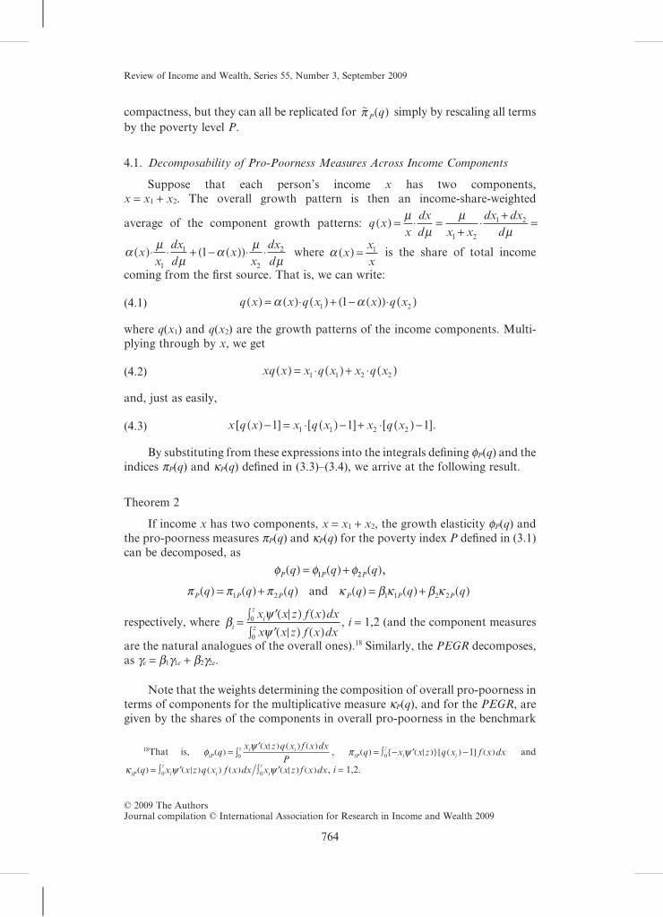
Figure 2 shows the observed and benchmark growth patterns for Indonesiafor the 1996–99 period. The curve representing the actual growth pattern liesentirely below the benchmark for all percentiles way past the headcount ratio(50.49 percent). In fact, the growth patterns for all other sub-periods (not shownhere) also lie below the benchmark, meaning that growth was unambiguouslyanti-poor in those other cases, but the 1996–99 period requires a different inter-pretation, since aggregate expenditure fell over that period. Namely, the expendi-tures of the poor fell by less than the average during the recession, which countsas a pro-poor growth experience. In all other sub-periods, economic growth inIndonesia in the 1990s was not pro-poor in the sense defined in this paper: positiveeconomic growth did not deliver a significant reduction in poverty, where the levelof significance is set at the amount of poverty reduction that would have beenachieved under distributional neutrality.

To further illustrate this point empirically, we computed our additive measureof pro-poorness pP(q) for the headcount index, Watts index, normalized povertydeficit and squared poverty gap. The estimates, presented in Table 3, are calculatedusing the growth patterns already described. It is clear from these results that in the1990s economic growth has not been significantly pro-poor in Indonesia. This

22SUSENAS stands for Survei Sosial Ekonomi Nasional (National Socio-Economic HouseholdSurvey), and BPS stands for Badan Pusat Statistik (Central Bureau of Statistics).

0.4

0.8

1.2

1.6

2.0

2.4

2.8

3.2

3.6

4.0

0 10 20 30 40 50 60 70 80 90 100

Cumulative percentage of the population

Gro

wth

rat

es

Benchmark

Actual

Figure 2. Growth Patterns (normalized growth incidence curves), 1996–99



769

conclusion holds for all sub-periods with positive growth and all poverty measures.This could be expected from Theorem 4, since the observed growth pattern curvesfor these periods lie below the benchmark.

Another empirical illustration of our theoretical results involves the compu-tation of the ratio measures kP(q) which are the correction factors associated withthe PEGR (see equation (3.6)). The results are presented in Table 4. The adjust-ment factor is less than one for all periods associated with positive growth, con-firming that growth was generally not pro-poor in Indonesia in the 1990s.

The interpretation of the results presented in Tables 3 and 4 follows the samelogic as for the numerical example involving Denmark and Portugal discussedearlier. The period 1996–99 deserves special attention because this is a period ofnegative growth. Per capita expenditure fell by about 8.6 percent on average in realterms. All additive measures of pro-poorness presented in Table 3 are positivewhile all the ratio measures in Table 4 are greater than one. According to ouranalytics, this means that the negative growth experienced in 1996–99 was actuallypro-poor—in the sense that the expenditure reductions experienced by the poorwere less than the mean reduction, and accordingly the benchmark increase inpoverty was greater than the actual increase in poverty. For instance, the additivepro-poorness value associated with the Watts index is equal to 0.44. The underly-ing elasticities are fw(q0) = -2.5587 and fw(q) = -0.3060. In other words, for every1 percent decrease in per capita expenditure, a distributionally-neutral processwould have increased poverty by 0.44 percent more than the observed pattern. Interms of the ratio pro-poorness measure (Kakwani et al.’s adjustment factor), wemay say that distributionally neutral growth would have increased poverty 8.36times faster than the observed outcome.23

23These conclusions can be confirmed by considering the results of a Shapley decomposition ofpoverty outcomes into their growth and distributional components over the period. See Essama-Nssahand Lambert (2006) for further details, and Kakwani (2000) for an axiomatic treatment establishing thesufficiency of pure growth and inequality effects to determine the overall effect on poverty as a sum.

TABLE 3

Additive Measures of Pro-Poorness for the 1990s

Headcount Poverty Gap Squared Poverty Gap Watts

1993–96 -0.28 -0.16 -0.09 -0.231996–99 0.41 0.27 0.16 0.441999–2002 -0.12 -0.06 -0.04 -0.021993–2002 -0.23 -0.16 -0.09 -0.22


TABLE 4

Ratio Measures of Pro-Poorness (correction factors for the PEGR) for the 1990s

Headcount Poverty Gap Squared Poverty Gap Watts

1993–96 0.64 0.62 0.62 0.631996–99 3.26 6.89 9.80 8.361999–2002 0.28 0.14 0.12 0.101993–2002 0.71 0.68 0.69 0.70




770

The available household survey data for 1999 and 2002 allow us to lookbeyond aggregate results for this period and consider the contribution of expen-diture components to the observed outcome. We also use the same data to look atpro-poorness at percentiles. Figure 3a shows the aggregate pattern of growth forthe period under consideration while Figure 3b represents a disaggregation of thisoverall pattern and is interpreted as the incidence of economic growth on five

0.7

0.8

0.9

1.0

1.1

1.2

1.3

1.4

10 20 30 40 50 60 70 80 90 100


Gro

wth

rat

es

Figure 3a. Aggregate Pattern of Growth (1999–2002)

-1.0

-0.5

0.0

0.5

1.0

1.5

2.0

2.5

10 20 30 40 50 60 70 80 90 100

Health

EducationOther non-food

Other food

Rice


Gro

wth

rat

es

Figure 3b. Incidence of Growth on Expenditure Components (1999–2002)



771

expenditure components: (1) rice, (2) other food, (3) education, (4) health, and (5)other non-food.24

Finally, we point to an interesting feature, apparent in the aggregate growthcurve (Figure 3a), which is further illuminated by resorting to our percentilemeasures. This growth curve crosses the benchmark case twice before the headcount ratio (55 percent). This means that we cannot use Theorem 4 to infer overallpro-poorness. However, the curve lies completely below the benchmark up to the20th percentile and between the 43rd and 55th percentiles. This represents about 60percent of the poor for whom expenditure per capita grew less than average. Theunderlying data show that for this segment of the poor population, on average, percapita expenditure grew 14 percent less than it would have, had growth beendistributionally neutral. The other 40 percent of the poor enjoyed an averageincrease in expenditure 17 percent above the hypothetical case. Figure 4 showsplots of pro-poorness at percentiles [pJ(q|p)] computed according to Theorem 3 forthree poverty measures. The fact that all these curves lie below zero indicates thateconomic growth has not been pro-poor at any percentile up to the headcount.Thus, according to our metric, the benefits enjoyed by the poor located betweenthe 20th and the 43rd percentiles are not high enough to compensate for the lossexperienced by those who came before.

Information on the contributions of expenditure components to pro-poornessis contained in Table 5. This tells us that the outcome in Figure 4 is driven mainlyby what happened to expenditure on rice, with some help from expenditure on

24The growth pattern curves presented in Figure 3a and 3b are more refined than those presentedin Figure 2: they are computed directly from household survey data (and smoothed using the Epanech-nikov kernel function) whilst the curves in Figure 2 come from a parameterization of the Lorenz curvebased on aggregate data.

-5

-4

-3

-2

-1

0

0 10 20 30 40 50 60 70 80 90 100

Watts

Poverty gap

Squared poverty gap


Figure 4. Pro-Poorness at Percentiles (1999–2002)



772

other food items. The underlying data reveal that rice represents 26 percent of totalexpenditure for the poor (total food expenditure including rice is about 73 percentof household expenditures for the poor). The growth pattern for rice in fact liesentirely below the benchmark, while that for the other food items lies below onlyfor the 20 percent poorest.

This important finding can be understood on the basis of the followingconsiderations. The 1997 currency crisis combined with rice crop reductioninduced by the drought and the Sumatra fires that occurred the same year led toskyrocketing prices for rice and other food. Between February 1996 and February1999 the price of rice increased by 184 percent. During the same period, foodinflation was estimated at 160 percent compared with 81 percent for non-fooditems (Suryahadi et al., 2003). Indonesia is the world’s largest net rice importer (18percent of the world’s total imports between 1998 and 2001). Since the financialcrisis, the government has increasingly sought to limit rice imports using both tariffand non-tariff barriers (such as licensing and temporary bans). From about 2000until late 2004, it is estimated that the domestic price of rice has settled around40–50 percent above the import price. This level is above any reached in theprevious three decades (Warr, 2005).

6. Concluding Remarks

Poverty reduction is considered a fundamental objective of development, andhas become a metric for assessing the effectiveness of development interventions.Measuring the pro-poorness of a growth process is an exercise in social evaluation,the outcome of which hinges on the underlying value judgments. In this paper wehave examined the elasticity-based measurement of pro-poorness, using an ana-lytical framework with three key elements: (1) the definition of a growth pattern interms of the point elasticity of individual incomes or consumption expenditureswith respect to the mean; (2) the use of individual poverty contributions andmembers of the class of additively separable poverty measures in the constructionof a social evaluation criterion; and (3) the selection of the poverty reductionobtainable under distributional neutrality as the threshold that must be crossed inorder to declare a growth pattern pro-poor.

What emerges from the analysis in these terms is a full taxonomy of existingelasticity-based pro-poorness measures, and a new measure, expressible in bothlevel and percentage terms, along with a method to decompose overall pro-

TABLE 5

A Decomposition of Aggregate Measure pP(q) (1999–2002)

Headcount Watts Poverty Gap Squared Poverty Gap

Rice -0.185 -0.172 -0.124 -0.061Other food -0.020 0.033 0.029 0.011Education -0.006 0.004 0.003 0.002Health 0.017 0.008 0.006 0.003Other non-food 0.073 0.070 0.051 0.025Aggregate -0.122 -0.056 -0.035 -0.021




773

poorness across income sources, or components of consumption expenditure, andan adaptation of the entire methodology to permit the “local” measurement ofpro-poorness at percentile points in the distribution among the poor.

An application of this methodology to expenditure data for Indonesia for theperiod 1993–2002 shows that the reduction in expenditure poverty achieved overthat period remains generally far below what distributionally-neutral growthwould have produced. However the 1997 economic crisis must be consideredpro-poor, since the losses for the non-poor outweigh those sustained by the poor.These conclusions are robust to the choice of both a poverty measure amongmembers of the additively separable class, and a poverty line up to about 2 dollarsa day. The behavior of five categories of expenditure over the 1999–2002 periodsuggests that the weak performance is due mainly to changes in food expenditure.

Pro-poorness decompositions across income components can identify incomesources (for example, labor income) whose growth pattern may be anti-poor orweakly pro-poor, enabling government to put forward appropriate income-enhancing policies. The ultimate objective of pro-poor income-generating policiesmay well be to increase people’s expenditures, and pro-poorness decompositionsacross expenditure components clearly have a complementary role in aiding pro-poor policy design. For example, Besley and Kanbur (1988) discuss the targetingof food subsidies to alleviate poverty. Poverty alleviating policy and pro-poorpolicy are not quite the same thing. It is worth reminding ourselves at this pointthat pro-poorness has a “relative” dimension: a pro-poor policy need not favor thepoor “more than” the rich, but it does favor them relative to a benchmark situationin which the gains go in equal proportions to both the poor and the rich.

Klasen (2008) shows how to extend some of the tools of pro-poor growthmeasurement to non-income dimensions of poverty, and suggests that an absoluteapproach may be particularly suitable for this. He sees the lack of consideration byeconomists of non-income pro-poorness as “highly lamentable . . . and . . . quitecontrary to the spirit of the MDGs which consider non-income dimensions ofwell-being (particularly education, health, and gender equity) as being of equalimportance to income poverty” (p. 424). Klasen shows how Ravallion and Chen’sgrowth incidence curve can be adapted to non-income dimensions, and he alsoexplains the nature of the insights that can then be derived for measuring andmonitoring, as well for targeting and other policy priorities (see also Grosse et al.,2008).

We hope that our approach may open up other new lines of investigation, inwhich the analysis will be conducted in terms of the elemental function q(x) whichspecifies the growth pattern. Standard errors for the poverty measures used in thispaper are easy to calculate in simple random samples (Kakwani, 1993b); similarwork could hopefully also establish standard errors for q(x) and the pro-poornessmeasures pP(q) and kP(q). Foster and Szekely’s (2000) conception of pro-poornessuses a growth elasticity for the Atkinson (1970) inequality index, and this could becast in terms of the underlying q(x). Bourguignon (2003) suggests in respect ofpro-poorness that “instead of considering poverty measures, it would be interest-ing to consider aggregate measures of social welfare” (p. 25); that could also bedone. Bourguignon gives encouragement for using the micro-level ingredient q(x)in the determination of pro-poorness: “the sooner poverty specialists will get used



774

to dealing systematically with distribution data, rather than with inequality orpoverty summary measures, at the national level, the better it will be” (p. 19).

We conclude with a remark that is prompted by a recent and very elegantanalysis of pro-poorness by Grimm (2007). All of the measures discussed in thispaper have in common that they are based on the anonymity axiom, because theelemental function q(x) (equivalently, the growth incidence curve of Ravallion andChen, 2003) describing the pattern of income growth takes no account of who is atwhat income level x before and after the growth experience (recall our equation(2.6)). As Grimm points out, the same growth pattern could reflect ongoing(chronic) poverty or transient poverty, depending on mobility among the poor. Headvocates “looking at . . . group-specific trajectories” (Grimm, 2007, p. 180), anddefines a modified growth incidence curve, à la Ravallion and Chen but defined forthe individuals who started at a specific percentile. He shows how, by using thiscurve, one can decompose changes in the Watts index into components accountedfor by income changes among the initially poor who crossed the poverty line, theinitially poor who did not cross the poverty line, and the initially non-poor whocrossed the poverty line (see also Jenkins and Van Kerm, 2006). Here is a domainin which the careful refinement of the q(x) modeling of this paper could have asignificant pay-off.

Appendix: Mathematical Results

Let U u x f x dxmx= ∫ ( ) ( )0 be the average of an attribute u(x) across the popula-

tion. Now let mean income m grow by a small amount Dm, so that individual income

x grows to x q x x x1+ ( )⋅⎡⎣⎢

⎤⎦⎥= +Δ Δμ

μ, say. The income value x + Dx now occurs

with frequency density f(x), and U changes to U U u x x f x dxmx+ = ∫ +( ) ( )Δ Δ0 .

Writing u x x u x u x x u x xu x q x+( ) = ( ) + ′( ) = ( ) + ′( ) ( )⋅Δ ΔΔμμ

, we have

Δ ΔU xq x u x f x dxmx= ⋅∫ ( ) ′( ) ( )μ

μ 0 , or:

μμUU xq x u x f x dx

u x f x dx

m

m

x

x⋅ =

( ) ′( ) ( )

( ) ( )

∫∫

ΔΔ

0

0

.(A.1)

Putting u(x) = x and U = m in (A.1), 1 0

0

=∫ ( ) ( )

∫ ( )

m

m

x

x

xq x f x dxxf x dx

which reduces to equa-

tion (2.3). For Theorem 1, just put u(x) = y(x|z) in (A.1). Equations (3.3) and (3.4)follow directly.

For the effect on the headcount H of a growth pattern q(x), let H → H* whenall incomes grow according to the growth pattern q(x), so that H = F(z). Let

x xq xy

yv x+ ( ) = ( )Δ

, assumed increasing in x, so that growth does not cause

reranking of income units, and let w be the inverse function of v, also increasing.



775

Then H* = F(w(z)) and φμ μ

μμ

μ μH qH H H

F w z F z

F z( ) = −( )

=( )( ) − ( )[ ]

( )→ →lim limΔ ΔΔ

Δ0 0

*. Set

w(z) = w0, so that z w w q w= + ( )0 0 0

Δμμ

. Then φ

μμ

μμ

μH qw q w f w

F z( ) =

− ( ) ( )⎡⎣⎢

⎤⎦⎥

( )→limΔ

ΔΔ

0

0 0 0

= −( ) ( )zq z f zH

since w0 → z as Dm → 0.

For Theorem 3, let p = F(t) � [0, 1] and define U t u x f x dxt( ) = ∫ ( ) ( )0 . Arguing

as before, the change in U(t) is Δ ΔU t xq x u x f x dxt( ) = ⋅∫ ( ) ′( ) ( )μ

μ 0 , so that:

μμU t

U t xq x u x f x dx

u x f x dx

t

t( )⋅

( )=

( ) ′( ) ( )

( ) ( )

∫∫

ΔΔ

0

0

.(A.2)

Putting u(x) = x in (A.2), so that U(t) = mL(p) where L(p) is the Lorenz curve, wehave

μμ

μL p

dL pd

x q x f x dxt

( )⋅

( )= ( ) −[ ] ( )∫ 1

0

.(A.3)

By the same token, with u xxp

( ) = , so that U tL p

pp( ) =

( )= ( )μ μ , (A.2) yields

μμ

μμp

d pd

xq x f x dx

xf x dx

t

t( )⋅

( )=

( ) ( )∫( )∫

0

0

.(A.4)

Property (2.4) tells us that the function of p (or x) defined in (A.3) has aninverted U-shape, and is zero at each end of its range, implying inequality reduc-tion, as claimed of property (2.4).

Now put u(x) = y(x|z) and U(t) = JP(p) in (A.2). The growth elasticity of JP(p)

is ζψ

P

t

P

q pxq x x z f x dx

J p( ) =

∫ ( ) ′( ) ( )( )

0 , from which Theorem 3 follows using note 18.

Son’s gS(p) is defined asd p

pμμ

( )( )

which is just γ μμ

= dtimes kTIP(q | p) from (A.4).

For Theorem 4, if pJ(q|p) > 0 "p � p0 then, as a function of t�[0, 1],∫ − ′( ){ } ( ) −[ ] ( )0 1

tx x z q x f x dxψ is initially upward-sloping. Taking the derivative,

$v < z : q(x) > 1 "x�[0, v]. Conversely, if $v < z : q(x) > 1 "x � [0, v], then∫ − ′( ){ } ( ) −[ ] ( )0 1

tx x z q x f x dxψ is initially upward-sloping, whence $p0 < 1 :

pJ(q|p) > 0 "p � p0. The result follows.Finally, using the deprivation function for D given in note 8 and the feasibility

property (2.3), (3.3)–(3.4) imply that πD z

mq

zx q x f x dxx( ) = − ∫ ( ) −[ ] ( )1

1 . Setting



776

q(x) = q* "x > z in this, and noting that ∫ ( ) =z

mx xf x dx μθ , we have1− ⋅ = ( )q

zqD

* μθ π , from which Theorem 5 follows.

References

Atkinson, Anthony B., “On the Measurement of Inequality,” Journal of Economic Theory, 2, 244–63,1970.

———, “On the Measurement of Poverty,” Econometrica, 55, 749–64, 1987.Besley, Timothy and Ravi Kanbur, “Food Subsidies and Poverty Alleviation,” The Economic Journal,

98, 701–19, 1988.Besley, Timothy, Robin Burgess, and Berta Esteve-Volart, “The Policy Origins of Poverty and Growth

in India,” in Timothy Besley and Louise Cord (eds), Delivering on the Promise of Pro-Poor Growth,Palgrave, New York, 2006.

Bourguignon, Francois, “The Growth Elasticity of Poverty Reduction: Explaining HeterogeneityAcross Countries and Time Periods,” in Theo S. Eicher and Stephen J. Turnovsky (eds), Inequalityand Growth: Theory and Policy Implications, MIT Press, Cambridge, MA, 3–26, 2003.

Chenery, Hollis, Móntele S. Ahluwalia, Clive L. G. Bell, John H. Duloy, and Richard Jolly, Redistri-bution with Growth: Policies to Improve Income Distribution in Developing Countries in the Contextof Economic Growth, Oxford University Press, New York and Oxford, 1974.

Datt, Gaurav, “Computational Tools for Poverty Measurement and Analysis,” International FoodPolicy Research Institute (IFPRI) Discussion Paper No. 50 (Food Consumption and NutritionDivision), Washington, DC, 1998.

Duclos, Jean-Yves, “What is Pro-Poor?” Social Choice and Welfare, 32, 37–58, 2009.Essama-Nssah, Boniface, “A Unified Framework for Pro-Poor Growth Analysis,” Economics Letters,

89, 216–21, 2005.Essama-Nssah, Boniface and Peter J. Lambert, “Measuring the Pro-Poorness of Income Growth

Within an Elasticity Framework,” Economics Discussion Paper No. 2006-12, University ofOregon, and Policy Research Working Paper No. WPS 4035, World Bank, 2006.

Foster, James E. and Miguel Szekely, “How Good is Growth?” Asian Development Review, 18, 59–73,2000.

Foster, James, Joel Greer, and Erik Thorbecke, “A Class of Decomposable Poverty Measures,”Econometrica, 52, 761–6, 1984.

Grimm, Michael, “Removing the Anonymity Axiom in Assessing Pro-Poor Growth,” Journal ofEconomic Inequality, 5, 179–97, 2007.

Grosse, Melanie, Kenneth Harttgen, and Stephan Klasen, “Measuring Pro-Poor Growth in Non-Income Dimensions,” World Development, 36, 1027–47, 2008.

Jenkins, Stephen P. and Peter J. Lambert, “Three ‘I’s of Poverty Curves, with an Analysis of U.K.Poverty Trends,” Oxford Economic Papers, 49, 317–27, 1997.

Jenkins, Stephen P. and Philippe Van Kerm, “Trends in Income Inequality, Pro-Poor Income Growth,and Income Mobility,” Oxford Economic Papers, 58, 531–48, 2006.

Kakwani, Nanak, “Poverty and Economic Growth with Application to Côte d’Ivoire,” The Review ofIncome and Wealth, 39, 121–38, 1993a.

———, “Measuring Poverty: Definitions and Significance Tests with Application to Côte d’Ivoire,” inM. Lipton and J. Van Der Gaag (eds), Including the Poor, The World Bank, Washington, DC,1993b.

———, “Measurement of Tax Progressivity: An International Comparison,” The Economic Journal,87, 71–80, 1977.

———, “On Measuring Growth and Inequality Components of Poverty with Application toThailand,” Journal of Quantitative Economics, 16, 67–80, 2000.

———, Methods in Measuring Poverty Matter: An Indian Story, One Pager Number 2, InternationalPoverty Center, Brazil, 2004.

Kakwani, Nanak and Ernesto M. Pernia, “What is Pro-Poor Growth?” Asian Development Review, 18,1–16, 2000.

Kakwani, Nanak and Hyun H. Son, “Pro-Poor Growth: Concepts and Measurement with CountryCase Studies,” Pakistan Development Review, 42, 417–44, 2003.

———, “On Assessing Pro-Poorness of Government Programmes: International Comparisons,” inNanak Kakwani and Jacques Silber (eds), Many Dimensions of Poverty, Palgrave Macmillan,Basingstoke and New York, 251–74, 2008a.

———, “Poverty Equivalent Growth Rate,” The Review of Income and Wealth, 54, 643–55, 2008b.



777

Kakwani, Nanak, Shahid Khandker, and Hyun H. Son, “Pro-Poor Growth: Concepts and Measure-ment with Country Case Studies,” Working Paper Number 2004-1, International Poverty Center,Brazil, 2004.

Kakwani, Nanak, Marcelo Neri, and Hyun H. Son, “Linkages Between Pro-Poor Growth, SocialProgrammes and the Labour Market: The Recent Brazilian Experience,” Working Paper No. 26,International Poverty Centre, Brazil, 2006.

Kalwij, Adriaan and Arjan Verschoor, “Not by Growth Alone: The Role of the Distribution of Incomein Regional Diversity in Poverty Reduction,” European Economic Review, 51, 805–29, 2007.

Klasen, Stephan, “Economic Growth and Poverty Reduction: Measurement Issues Using Income andNon-Income Indicators,” World Development, 36, 420–45, 2008.

Klasen, Stephan and Mark Misselhorn, “Determinants of the Growth Semi-Elasticity of PovertyReduction,” No. 15 Proceedings of the 2006 German Development Economics Conference, Berlin,2006.

Kraay, Aart, “When is Growth Pro-Poor? Evidence From a Panel of Countries,” Journal of Develop-ment Economics, 80, 198–227, 2006.

Lambert, Peter J., “Non-Equiproportionate Income Growth, Inequality and the Income Tax,” PublicFinance/Finances Publiques, 39, 104–18, 1984.

———, “Positional Equity and Equal Sacrifice: Design Principles for an EU-Wide Income Tax?” inMarc Fleurbaey, Maurice Salles, and John A. Weymark (eds), Social Ethics and NormativeEconomics, Studies in Choice and Welfare series, Springer, forthcoming, 2009.

McCulloch, Neil and Bob Baulch, Tracking Pro-Poor Growth: New Ways to Spot the Biases andBenefits, ID21 Insights No. 31, Institute of Development Studies, Sussex, 2000.

McKinley, Terry, How Inclusive is “Inclusive Growth”? Development Viewpoint No. 6, School ofOriental and African Studies, London, 2008.

Osmani, Siddiq, Defining Pro-Poor Growth, One Pager Number 9, International Poverty Center, Brazil,2005.

Ravallion, Martin, “Issues in Measuring and Modelling Poverty,” The Economic Journal, 106, 1328–43,1996.

———, Defining Pro-Poor Growth: A Response to Kakwani, One Pager Number 4, InternationalPoverty Center, Brazil, 2004.

Ravallion, Martin and Shaohua Chen, “What Can New Survey Data Tell Us About Recent Changesin Distribution and Poverty?” World Bank Economic Review, 11, 357–82, 1997.

———, “Measuring Pro-Poor Growth,” Economics Letters, 78, 93–9, 2003.Shorrocks, Anthony F., “Deprivation Profiles and Deprivation Indices,” in Stephen Jenkins, Arie

Kapteyn, and Bernard Van Praag (eds), The Distribution of Welfare and Household Production:International Perspectives, Cambridge University Press, Cambridge, 250–67, 1998.

Son, Hyun H. “A Note on Pro-Poor Growth,” Economics Letters, 82, 307–14, 2004.———, “Assessing the Pro-Poorness of Government Fiscal Policy in Thailand,” Public Finance

Review, 34, 427–49, 2006.Suryahadi, Asep, Sudarno Sumarto, and Lant Pritchett, “Evolution of Poverty During the Crisis in

Indonesia,” Asian Economic Journal, 17, 221–41, 2003.Warr, Peter G., “Food Policy and Poverty in Indonesia: A General Equilibrium Analysis,” Australian

Journal of Agricultural and Resource Economics, 49, 429–51, 2005.Watts, Harold, “An Economic Definition of Poverty,” in Daniel P. Moynihan (ed.), On Understanding

Poverty: Perspectives from the Social Sciences, Basic Books, New York, 316–29, 1968.World Bank, Indonesia: Improving Efficiency and Equity—Changes in the Public Sector’s Role, Report

No. 14006-IND, Country Department III, East Asia and Pacific Region, The World Bank,Washington, DC, 1995.

———, Indonesia: Dimensions of Growth, Report No. 15383-IND, Country Department III, East Asiaand Pacific Region, The World Bank, Washington, DC, 1996.

———, World Development Report 2000/2001: Attacking Poverty, The World Bank and Oxford Uni-versity Press, Washington, DC and New York, 2001.

Zepeda, Eduardo, Pro-Poor Growth: What is it? One Pager Number 1, International Poverty Center,Brazil, 2004.



778

by ssama ssah and eter ambert - Review of Income and Wealth · policies to induce higher growth...

Documents

Transcript of by ssama ssah and eter ambert - Review of Income and Wealth · policies to induce higher growth...