By Michael Su

04/16/2009

Introduction Fluid characteristics Navier-Stokes equation Eulerian vs. Lagrangian approach Dive into the glory detail (A case study of the

2d fluid simulation) Advection Diffusion Pressure solve

Fluid object couple One-way and two-way coupling

Real-time fluids

Broad view of the fluid simulation in graphics community and its potential applications

Basic knowledge about the grid-based fluid simulation

Understanding the challenges of the existing methods

Foundation for the following two fluids- related lectures (smoke & granular material).

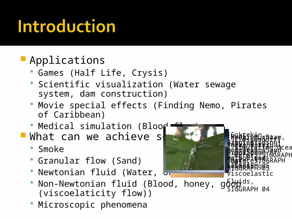
Applications Games (Half Life, Crysis) Scientific visualization (Water sewage system, dam

construction) Movie special effects (Finding Nemo, Pirates of

Caribbean) Medical simulation (Blood flow)

What can we achieve so far? Smoke Granular flow (Sand) Newtonian fluid (Water, ocean) Non-Newtonian fluid (Blood, honey, goop

(viscoelaticity flow)) Microscopic phenomena

[Zhu, Bridson]Animating Sand as a Fluid, SIGGRAPH 05

[Fedkiw, Stam, Jensen] Visual Simulation of Smoke, SIGGRAPH 01

[Tessendorf] Simulating Ocean Water, SIGGRAPH 01

[Goktekin, Bargteil, O'Brien] A Method for Animating Viscoelastic Fluids,SIGGRAPH 04

[Wang, Mucha, Turk] Water Drops on Surfaces, SIGGRAPH 05

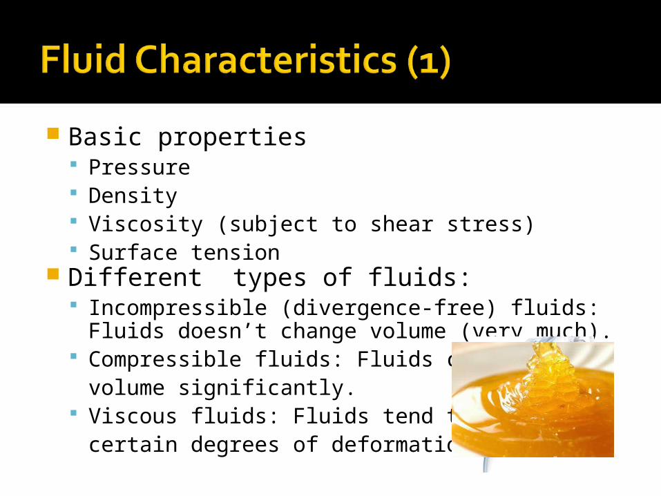
Basic properties Pressure Density Viscosity (subject to shear stress) Surface tension

Different types of fluids: Incompressible (divergence-free) fluids: Fluids

doesn’t change volume (very much). Compressible fluids: Fluids change their

volume significantly. Viscous fluids: Fluids tend to resist a

certain degrees of deformation

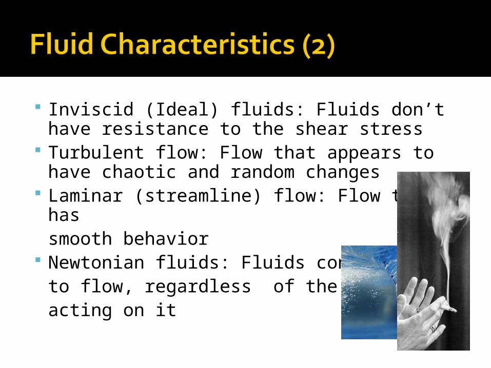
Inviscid (Ideal) fluids: Fluids don’t have resistance to the shear stress

Turbulent flow: Flow that appears to have chaotic and random changes

Laminar (streamline) flow: Flow that hassmooth behavior

Newtonian fluids: Fluids continueto flow, regardless of the force acting on it

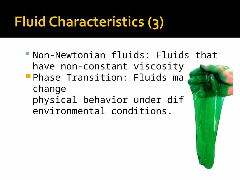
Non-Newtonian fluids: Fluids that have non-constant viscosity

Phase Transition: Fluids may change physical behavior under different environmental conditions.

Modeling continuum fluids on discrete systems – It’s all about approximations

Topological variations and different kinds of behaviors with interacting subjects

Numerical stabilities, accuracy and convergence issues

PerformanceUser control

By Michael Su

04/20/2009

Calculus Review (1)

Gradient ( ): A vector pointingin the direction of the greatest rate of increment

Divergence ( ): Measure how the vectors are converging or diverging at a given location (volume density of the outward flux)

z

u

y

u

x

uu ,,

u can be a scalar or a vector

zyx

uuu

u u can only be a vectorSource, Div(u) > 0

Sink, Div(u) < 0

z

u

y

u

x

uu ,,

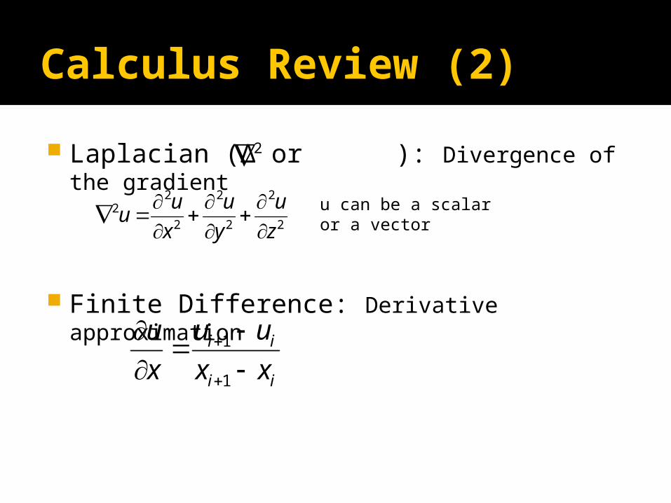
Calculus Review (2)

Laplacian (∆ or ): Divergence of the gradient

Finite Difference: Derivative approximation

2

2

2

2

2

2

22

z

u

y

u

x

uu

u can be a scalar or a vector

ii

ii

xx

uu

x

u

1

1

Momentum equation

Incompressibility Claude-Louis Navier (1785~1836)

George Gabriel Stokes (1819~1903)

ut = k2u –(u)u – p + f

u=0

Change in velocity

Diffusion/Viscosity

Advection Pressure Body Forces

u: the velocity fieldk: kinematic viscosity

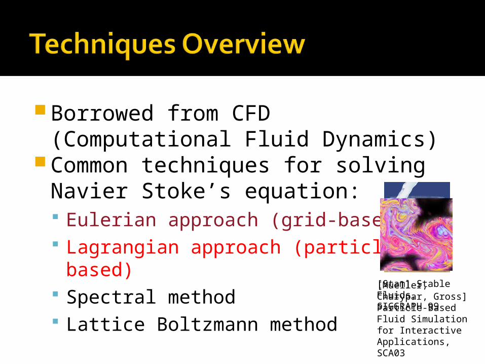
[Mueller, Charypar, Gross] Particle-Based Fluid Simulation for Interactive Applications, SCA03

Borrowed from CFD (Computational Fluid Dynamics)

Common techniques for solving Navier Stoke’s equation: Eulerian approach (grid-based) Lagrangian approach (particle-based) Spectral method Lattice Boltzmann method

[Stam] Stable Fluids, SIGGRAPH 99

Discretize the domain using finite differences

Define scalar & vector fields on the gridUse the operator splitting

technique to solve each term separately

Evaluation: Derivative approximation

Adaptive time step/solver Memory usage & speed

Grid artifact/resolution limitation

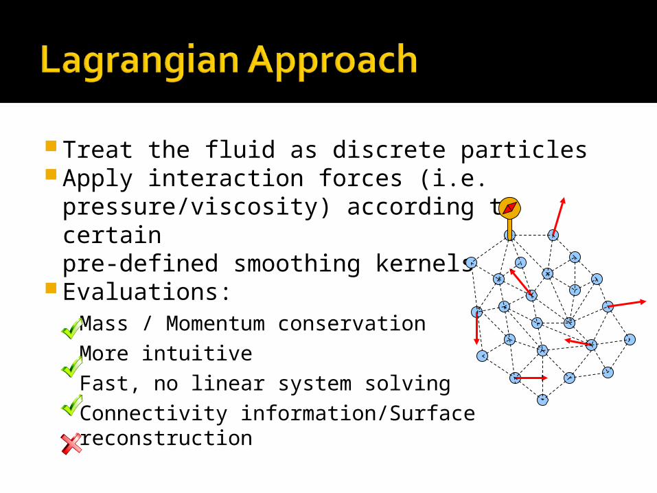
Treat the fluid as discrete particlesApply interaction forces (i.e.

pressure/viscosity) according to certain pre-defined smoothing kernels

Evaluations:Mass / Momentum conservationMore intuitiveFast, no linear system solvingConnectivity information/Surface reconstruction

Case Study: A 2D Fluid Simulator

We focus exclusively on incompressible, viscous fluid

Assuming the gravity is the only external force

No inflow or outflow Constant viscosity, constant density

everywhere in the fluid

Scalar/Vector fields defined on the grid

Advection Body Force Diffusion

Pressure Solve

ut = k2u –(u)u – p + fu=0

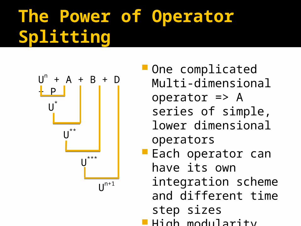
The Power of Operator Splitting

Un + A + B + D + P

U*

U**

U***

Un+1

One complicated Multi-dimensional operator => A series of simple, lower dimensional operators

Each operator can have its own integration scheme and different time step sizes

High modularity and easy to debug

Sometimes called “Convection” or “Transport” Define how a quantity moves with the

underlying velocity field This term ensures the conservation of

momentum Advection equation:

Approaches: Forward Euler (unstable) Semi-Lagragian advection (stable for large time

steps, but suffers from the dissipation issue)

)( uuut

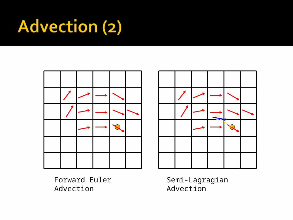
Forward Euler Advection Semi-Lagragian Advection

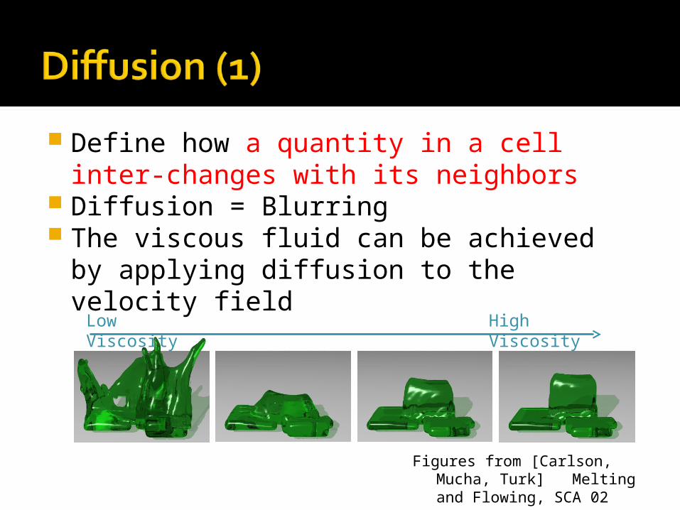
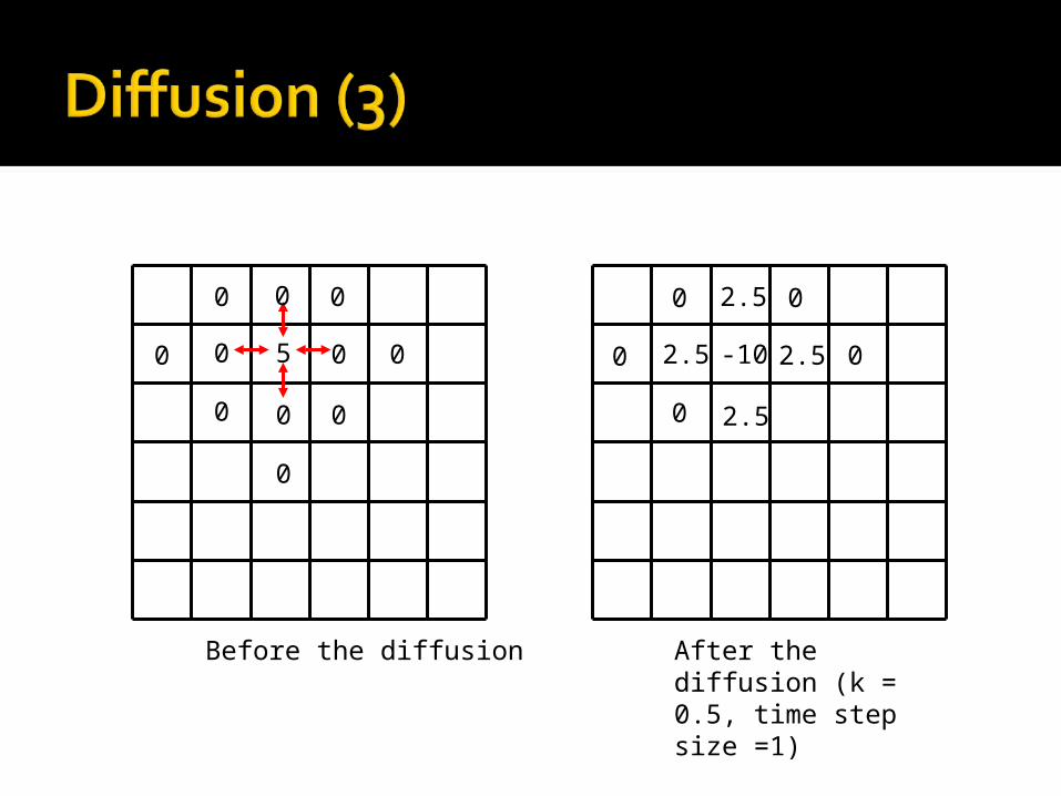
Define how a quantity in a cell inter-changes with its neighbors

Diffusion = Blurring The viscous fluid can be achieved by

applying diffusion to the velocity field

Low Viscosity High Viscosity

Figures from [Carlson, Mucha, Turk] Melting and Flowing, SCA 02

Diffusion equation:

Approaches: Explicit formulation

Implicit formulation (for high viscosity)

)4( ,1,1,,1,1 jijijijijit uuuuutku

ukut2

)4( ,1

1,1

1,1

,11

,11

,1

, jin

jin

jin

jin

jin

jin

jin uuuuutkuu

1 1

1

1

-4

Unknowns

50 0

0

0

0

0

0 0

0

0

0

-102.5 2.5

2.5

0

0

0 0

0

2.5

Before the diffusion After the diffusion (k = 0.5, time step size =1)

It’s sometimes called “Pressure Projection”

What does the pressure do? Keep the fluid at constant volume

(incompressible, conservation of mass). Make sure the velocity field stays

divergence-free

€

fluxall _ faces

∑ = 0

CompressibleIncompressible

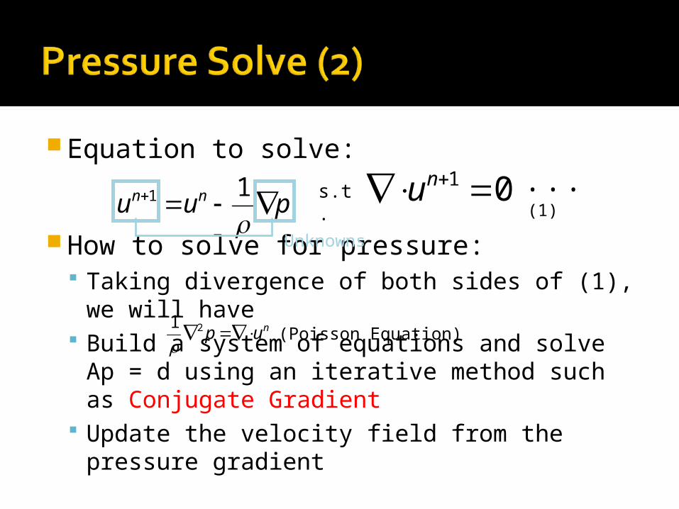
puu nn

11

Equation to solve:

How to solve for pressure: Taking divergence of both sides of (1), we

will have Build a system of equations and solve Ap =

d using an iterative method such as Conjugate Gradient

Update the velocity field from the pressure gradient

nup 21

01 nus.t. • • • (1)

Unknowns

(Poisson Equation)

What about the pressure on boundary nodes? Free surface: The fluid can evolve freely (p = 0) Solid wall: The fluid can’t penetrate the wall but can flow freely in tangential

directions (Neumann BC)

Free surface

Solid wall

€

uboundary ⋅n = usolid ⋅n

Possible reasons why your simulation doesn’t look right: CFL condition violation

=> Smaller time steps / Implicit solver Flux conservation => BCs may not be set correctly Grid resolution/ Memory => Adaptive grids Numerical dissipation => Back and Forth Error

Compensation and Correction [4] / Vorticity confinement [5]

Handle the interface and complex topological changes => Level set method [6]

Volume loss => Particle level set [7]

€

t ⋅u ≤ C ⋅Δx

One-way coupling: Solid-Fluid interaction: The fluid has no

influence on the solid Fluid-Solid interaction: The solid has no

influence on the fluid Two-way coupling:

Manipulate the boundary conditions Finite Element techniques: ALE & DLM Rigid Fluid: Treat the solid as fluids and

enforce the rigidity constraint [8]

Principles: Cheap to compute Low memory consumption Stability Plausibility Interactivity

Common techniques: Procedural water: Superimpose sine waves

of a variety of amplitudes and directions. [9]

Real-time Fluids (2)

Heightfield approximations: If the surface is the only interest, it can be represented using a 2d heightfield and animated by 2d wave equations with interaction forces.

Particle systems: This approach is

good at simulating a small amount of water such as a puddle, a bubble, or splashing fluids

H(x, y)

€

f (x i,x j ) =k1

x i − x jm −

k2

x i − x jn

⎛

⎝

⎜ ⎜

⎞

⎠

⎟ ⎟⋅x i − x jx i − x j

[1] R. Bridson and M. Müller-Fischer. Fluid Simulation. SIGGRAPH 07 Course Notes

[2] R. Bridson. Fluid Simulation for Computer Graphics. A K Peters, 2008

[3] J. Stam. Real-Time Fluid Dynamics for Games. GDC 2003 [4] B. Kim, Y. Liu, I. Llamas, and J. Rossignac. FlowFixer:

Using BFECC for Fluid Simulation. EGWNP 05 [5] R. Fedkiw, J. Stam, and H.W. Jenson. Visual Simulation of

Smoke. SIGGRAPH 01 [6] N. Foster, R. Fedkiw, Practical Animation of Liquids.

SIGGRAPH 01 [7] D. Enright, S. Marschner, R. Fedkiw. Animation and

Rendering of Complex Water Surfaces. SIGGRAPH 02 [8] M. Carlson, P. J. Mucha, G. Turk. Rigid Fluid: Animating

the Interplay Between Rigid Bodies and Fluid. SIGGRAPH 04

References (2)

[9] D. Hinsinger, F. Neyret, M. Cani. Interactive Animation of Ocean Waves. SCA 02