A Comparison of Lagrangian/Eulerian Approaches for ...
60
SANDIA REPORT SAND2009-5154 Unlimited Release Printed September 2009 A Comparison of Lagrangian/Eulerian Approaches for Tracking the Kinematics of High Deformation Solid Motion Allen C. Robinson, David I. Ketcheson, Thomas L. Ames, Grant V. Farnsworth Prepared by Sandia National Laboratories Albuquerque, New Mexico 87185 and Livermore, California 94550 Sandia is a multiprogram laboratory operated by Sandia Corporation, a Lockheed Martin Company, for the United States Department of Energy’s National Nuclear Security Administration under Contract DE-AC04-94-AL85000. Approved for public release; further dissemination unlimited.
Transcript of A Comparison of Lagrangian/Eulerian Approaches for ...

SANDIA REPORTSAND2009-5154Unlimited ReleasePrinted September 2009
A Comparison of Lagrangian/EulerianApproaches for Tracking theKinematics of High Deformation SolidMotion
Allen C. Robinson, David I. Ketcheson, Thomas L. Ames, Grant V. Farnsworth
Prepared bySandia National LaboratoriesAlbuquerque, New Mexico 87185 and Livermore, California 94550
Sandia is a multiprogram laboratory operated by Sandia Corporation,a Lockheed Martin Company, for the United States Department of Energy’sNational Nuclear Security Administration under Contract DE-AC04-94-AL85000.
Approved for public release; further dissemination unlimited.

Issued by Sandia National Laboratories, operated for the United States Department ofEnergy by Sandia Corporation.
NOTICE: This report was prepared as an account of work sponsored by an agency ofthe United States Government. Neither the United States Government, nor any agencythereof, nor any of their employees, nor any of their contractors, subcontractors, or theiremployees, make any warranty, express or implied, or assume any legal liability or re-sponsibility for the accuracy, completeness, or usefulness of any information, appara-tus, product, or process disclosed, or represent that its use would not infringe privatelyowned rights. Reference herein to any specific commercial product, process, or serviceby trade name, trademark, manufacturer, or otherwise, does not necessarily constituteor imply its endorsement, recommendation, or favoring by the United States Govern-ment, any agency thereof, or any of their contractors or subcontractors. The views andopinions expressed herein do not necessarily state or reflect those of the United StatesGovernment, any agency thereof, or any of their contractors.
Printed in the United States of America. This report has been reproduced directly fromthe best available copy.
Available to DOE and DOE contractors fromU.S. Department of EnergyOffice of Scientific and Technical InformationP.O. Box 62Oak Ridge, TN 37831
Telephone: (865) 576-8401Facsimile: (865) 576-5728E-Mail: [email protected] ordering: http://www.doe.gov/bridge
Available to the public fromU.S. Department of CommerceNational Technical Information Service5285 Port Royal RdSpringfield, VA 22161
Telephone: (800) 553-6847Facsimile: (703) 605-6900E-Mail: [email protected] ordering: http://www.ntis.gov/help/ordermethods.asp?loc=7-4-0#online
DEPA
RTMENT OF ENERGY
• • UN
ITED
STATES OF AM
ERIC
A

SAND2009-5154Unlimited Release
Printed September 2009
A Comparison ofLagrangian/Eulerian Approaches for
Tracking the Kinematics of HighDeformation Solid Motion
Allen C. Robinson, David I. Ketcheson,Thomas L. Ames, and Grant V. Farnsworth
Computational Shock & Multiphysics DepartmentSandia National Laboratories
MS-0378, P.O. Box 5800Albuquerque, NM 87185-0378
Abstract
The modeling of solids is most naturally placed within a Lagrangianframework because it requires constitutive models which depend onknowledge of the original material orientations and subsequent defor-mations. Detailed kinematic information is needed to ensure materialframe indifference which is captured through the deformation gradientF. Such information can be tracked easily in a Lagrangian code. Un-fortunately, not all problems can be easily modeled using Lagrangianconcepts due to severe distortions in the underlying motion. Eithera Lagrangian/Eulerian or a pure Eulerian modeling framework mustbe introduced. We discuss and contrast several Lagrangian/Eulerianapproaches for keeping track of the details of material kinematics.
3

Acknowledgments
The authors acknowledge helpful discussions, interactions and communica-tions with our colleagues including Rebecca Brannon, Kevin Brown, Christo-pher Garasi, Mark Christon, Greg Miller, Sharon Petney, Duane Labreche,William Scherzinger and Michael Wong. Ed Love pointed out the utility andform of the rotation preserving midstep interpolation formulae and kindlyreviewed a draft of this report.
The student intern program at Sandia provided opportunities for authorsAmes, Ketcheson and Farnsworth to provide contributions to this work.
Sandia is a multiprogram laboratory operated by Sandia Corporation,a Lockheed Martin Company, for the United States Department of En-ergy’s National Nuclear Security Administration under contract DE-AC04-94AL85000.
4

Contents
1 Introduction 9
2 Stretch and Rotation Update Method (VR) 12
2.1 VR Remap . . . . . . . . . . . . . . . . . . . . . . . . . . . . 15
3 Quaternion Representation VR Method (QVR) 22
3.1 QVR Remap . . . . . . . . . . . . . . . . . . . . . . . . . . . 24
4 Inverse Deformation Gradient Method (IDG) 26
4.1 DG Constrained Transport Remap . . . . . . . . . . . . . . . 26
5 Results for Given 2D Motions 33
5.1 Constant Velocity . . . . . . . . . . . . . . . . . . . . . . . . . 34
5.2 Sinusoidal Shear . . . . . . . . . . . . . . . . . . . . . . . . . . 35
5.3 Exponential Vortex . . . . . . . . . . . . . . . . . . . . . . . . 38
5.4 Diverging Flow . . . . . . . . . . . . . . . . . . . . . . . . . . 40
5.5 ABC Vortical Flow . . . . . . . . . . . . . . . . . . . . . . . . 42
6 Results for Given 3D Motions 45
6.1 3D Exponential Vortex . . . . . . . . . . . . . . . . . . . . . . 46
6.2 3D ABC Vortical Flow . . . . . . . . . . . . . . . . . . . . . . 48
7 A Three Dimensional Impact Problem 51
5

8 Conclusions 52
A Alternative Method For Calculating Exact Solutions 57
List of Figures
1 Stretch cutoff example for λs = 10−2 . . . . . . . . . . . . . . 18
2 Stretch cutoff example for λs = 10−1 . . . . . . . . . . . . . . 19
3 Stretch cutoff example for λs = 4 · 10−1 . . . . . . . . . . . . . 20
4 VR versus QVR rotation comparison . . . . . . . . . . . . . . 25
List of Tables
1 Lag. Constant Velocity CPU time comparison . . . . . . . . . 34
2 ALE Constant Velocity CPU time comparison . . . . . . . . . 35
3 Lag. Sinusoidal Shear stretch eigenvalue convergence rates . . 36
4 Lag. Sinusoidal Shear rotation matrix convergence rates . . . 36
5 ALE Sinusoidal Shear stretch eigenvalue convergence rates . . 36
6 ALE Sinusoidal Shear rotation matrix convergence rates . . . 37
7 Lag. Sinusoidal Shear CPU time comparison . . . . . . . . . . 37
8 ALE Sinusoidal Shear CPU time comparison . . . . . . . . . . 37
9 Lag. Exponential Vortex stretch eigenvalue convergence rates . 38
10 Lag. Exponential Vortex rotation matrix convergence rates . . 39
11 ALE Exponential Vortex stretch eigenvalue convergence rates 39
6

12 Lag. Exponential Vortex CPU time comparison . . . . . . . . 39
13 ALE Exponential Vortex CPU time comparison . . . . . . . . 40
14 Lag. Diverging Flow stretch eigenvalue convergence rates . . . 41
15 ALE Diverging Flow stretch eigenvalue convergence rates . . . 41
16 Lag. Diverging Flow CPU time comparison . . . . . . . . . . . 41
17 ALE Diverging Flow CPU time comparison . . . . . . . . . . 42
18 Lag. ABC Vortical Flow stretch eigenvalue convergence rates . 43
19 Lag. ABC Vortical Flow rotation matrix convergence rates . . 43
20 ALE ABC Vortical Flow stretch eigenvalue convergence rates . 44
21 ALE ABC Vortical Flow rotation matrix convergence rates . . 44
22 Lag. ABC Vortical Flow CPU time comparison . . . . . . . . 45
23 ALE ABC Vortical Flow CPU time comparison . . . . . . . . 45
24 Lag. 3D Exp. Vortex stretch eigenvalue convergence rates . . 46
25 ALE 3D Exp. Vortex stretch eigenvalue convergence rates . . 46
26 Lag. 3D Exp. Vortex rotation matrix convergence rates . . . . 47
27 ALE 3D Exp. Vortex rotation matrix convergence rates . . . . 47
28 Lag. 3D Exponential Vortex CPU time comparison . . . . . . 47
29 ALE 3D Exponential Vortex CPU time comparison . . . . . . 48
30 Lag. 3D ABC Vort. Flow stretch eigenvalue convergence rates 48
31 ALE 3D ABC Vort. Flow stretch eigenvalue convergence rates 49
32 Lag. 3D ABC Vort. Flow rotation matrix convergence rates . 49
33 ALE 3D ABC Vort. Flow rotation matrix convergence rates . 49
7

34 Lag. 3D ABC Vortical Flow CPU time comparison . . . . . . 50
35 ALE 3D ABC Vortical Flow CPU time comparison . . . . . . 50
36 3D impact test time comparison . . . . . . . . . . . . . . . . . 51
This page intentially left blank.
8

1 Introduction
A Lagrangian framework is ideal for modeling the response of solids to exter-nal loads because such modeling typically requires constitutive models whichdepend on detailed knowledge of the material motion. This relationshipis captured through the deformation gradient F. However, some motionscannot be described on a Lagrangian grid and Eulerian concepts must beintroduced. Arbitrary Lagrangian-Eulerian (ALE) codes accomplish this bytaking a Lagrangian step followed by an optional remap step.20 The La-grangian step solves the equations of motion in the frame of reference of themoving material. The Eulerian or remap step moves the mesh coordinatesback to their original configuration or to some other convenient position de-termined by the remesh step. Some approaches remap to nearby meshesusing conservative interpolation concepts from hyperbolic equations, and forthis reason, the remap step can be referred to as an advection step. Othertechnologies implement a remap step that is more general.
A pure Eulerian framework for solid dynamic modeling is also possible.The general approach is to write the equations in conservation form, analyzetheir relevant mathematical properties and then solve numerically. Equa-tions for elastic flow in Eulerian form are discussed by Plohr and Sharp.22
This work was subsequently extended to include rate-dependent and rate-independent plasticity.23 One-dimensional numerical solution techniques forthis type of model were later presented.37 The 20-component equation sys-tem for rate-dependent metals includes the inverse deformation gradient (9),momentum (3) and energy conservation (1), plastic strain (6) and a workhardening equation. (If the assumption of an initial uniform density is re-laxed then one more equation would be required for a total of 21 variables.)Application of these equations to shear band modeling has also been pre-sented.10 One of the difficulties of solid dynamics modeling is that the mosteffective and universal modeling framework and associated constitutive formshave not been completely agreed upon. Careful and thoughtful reasoningbased on physical principles and experimental data is required.21,36 Multi-dimensional modeling results from this group are relatively recent and areassociated with a front tracking numerical method.34,35 The issue of the useof stable, properly posed equations for the inverse deformation gradient isdiscussed briefly by Walter, et al.35 in relationship to an interface equation
9

and in detail by Miller and Colella.18,19
Trangenstein and Collella introduced a general framework for modelingfinite deformation in solids.30 Their paper details many of the difficulties ofmodeling finite deformation in solids in an Eulerian framework. Additionalpapers by Trangenstein and coauthors have also appeared.29,31,32 More re-cently, work by Miller and Collella discusses the stability requirements for theinverse deformation gradient equations in Eulerian form and presents bothelastic and elastic-plastic results.18,19 The model presented is very similarbut involves 24 independent variables because the plastic deformation gra-dient is solved for in place of the symmetric plastic strain and an additionalmass density equation is used.
Lin and Ballmann develop a conservative Godunov formulation based onthe solution of a Riemann problem for one-dimensional motion of a thin-walled tube with longitudinal and torsional stress wave propagation.16 Thesystem maintains longitudinal and circumferential velocities and strains asindependent degrees-of-freedom. A Godunov approach is also followed byUdaykumar, et. al.33 They solve a two-dimensional conservation law systemfor mass, momentum, energy, equivalent plastic strain and deviatoric stress.This system only keeps advective terms for the deviatoric stress in the con-servative flux leaving the elastic contributions to be discretized as sourceterms.
Fundamentally, solid dynamic modeling must include first, a descriptionof the kinematics of material motion; and second, an optional set of statevariables which may evolve with the motion and track local material stateproperties. Linear elastic or hyperelastic models provide the stress given in-formation about the current deformation. However, for large elasto-plasticdeformations, the stress in general depends on the history of the deformation.Hypoelastic models, which relate invariant stress rate measures to deforma-tion rates, have long been popular despite concerns about the thermodynamicvalidity of commonly used simple hypoelastic forms.28 This report toucheson an ALE formulation developed from a hypoelastic model point of view interms of the Green-Naghdi rate. All constitutive models are cast in the un-rotated configuration and the rotation tensor is used to transform the stressfrom the unrotated to the current configuration. The fundamental kinematicvariables related to the deformation gradient are evaluated at element cen-
10

ters. This is equivalent to the average value in the element to second orderin the element size. A conservative interpolation method is used to updateelement centered average values across a remap step. Thus, we effectivelysolve
φt + ∇ · (φvm) = 0
where φ is a scalar value and vm is the effective remesh velocity. In this doc-ument components of tensors are remapped individually. In the remap oper-ations, both the kinematic descriptors and state descriptors may be movedoff any constraint surface where they are supposed to lie. For example, thedeterminant of a deformation gradient must be positive in order to create aphysically relevant one-to-one mapping between each material point and itscurrent location. Furthermore, curls of gradients should vanish identically. Agiven remapping method may not preserve these properties, and the resultsmay not be desirable. As another example, it may be difficult to preserve astress state that is constrained to lie on a yield surface in the remap step.Issues associated with remap of material state information are difficult, andtradeoffs may be necessary.24
Any Eulerian or ALE scheme for tracking the kinematics of solid defor-mation is bound to eventually break down given enough deformation. Soliddynamics intrinsically depends on the one-to-one mapping between a ref-erence set of coordinates and the current coordinates. Because it is alwayspossible to generate a flow which is distorted enough that this mapping is dif-ficult or impossible to achieve, some sort of implicit or explicit regularizationor correction is required. Thus, it is essential to determine which techniquesare the most accurate and robust in the face of a variety of difficult materialmotions.
In this report we are concerned with understanding issues associated withthe choice of algorithms for modeling the kinematics of solid motion as well asthe consequences of these choices with respect to speed and accuracy. We willlay the state descriptor issue aside and concentrate on approaches for main-taining the kinematic information in the form of the deformation gradient orits inverse. We shall investigate a traditional approach for updating compo-nents of the polar decomposition, a more compact form based on quaternionsand an approach based on a direct computation of the inverse deformationgradient. We propose a few simple test problems with exact solutions andmake comparisons of the methods in Lagrangian and ALE frameworks.
11

2 Stretch and Rotation Update Method (VR)
We define the Lagrangian motion x(a, t), where x represents the currentcoordinates as a function of the initial Lagrangian positions a and time t, andthe corresponding velocity, v = x(a, t) = ∂x/∂t. Vector differential operators∇, ∇× and ∇· are always with respect to the specified spatial coordinates,x. Also, w is the axial vector corresponding to the skew-symmetric tensorW (i.e. Wu = w × u for every vector u). We assume a time step ∆t andmesh spacing ∆x.
The kinematics of modeling continuum solids is described via a motion,x(a, t), where x is the current position as a function of the initial Lagrangiancoordinates a and time t. Of particular interest is the deformation gradienttensor ∂x/∂a which is needed in order to properly compute material stressstates through the constitutive assumptions.
One common approach is to decompose the deformation gradient at theinitial time,
F =∂x
∂a= VR (2.1)
into a symmetric positive definite left stretch tensor V and an orthonormalrotation tensor R. The V and R matrices are then updated separately ina Lagrangian sense using a rate equation based on the mid-point velocitygradient tensor L.5,8, 14 That is,
Ln+1/2 = ∇n+1/2vn+1/2 = (∇v)n+1/2 (2.2)
and
Dn+1/2 =1
2(Ln+1/2 + LT
n+1/2) (2.3)
Wn+1/2 =1
2(Ln+1/2 − LT
n+1/2). (2.4)
An angular velocity (or spin) tensor Ω is calculated from Dn+1/2 and Vn
usingωn+1/2 = wn+1/2 + [tr(Vn)I − Vn]−1zn+1/2, (2.5)
where zn+1/2, wn+1/2 and ωn+1/2 are the axial vectors corresponding tothe skew-symmetric tensors Zn+1/2 = Dn+1/2Vn − VnDn+1/2, Wn+1/2 and
12

Ωn+1/2, respectively. A common first-order in time algorithm for Vn andRn,5,8 is
Vn+1 = Vn + ∆t(Ln+1/2Vn − VnΩn+1/2) (2.6)
Rn+1 = [I −1
2∆tΩn+1/2]
−1[I +1
2∆tΩn+1/2]Rn. (2.7)
Note that the right hand side of Equation 2.7 is an approximation to thematrix exponential solution
Rn+1 = exp[Ωn+1/2∆t]Rn.
which is exact if Ω is constant. The overall algorithm is first-order accuratebecause the derivative is computed using Vn instead of Vn+1/2 in Equation2.5.
For staggered space-time discretizations, the velocity gradient L is knownonly at the mid-point time, but the V and R tensors are known at the timestep. After obtaining Ωn, we can compute an estimate of V at the mid-pointtime using
Vn+1/2 = Vn +1
2∆t(Ln+1/2Vn − VnΩn) (2.8)
and then use this estimate of Vn+1/2 to compute Ωn+1/2 as in Equation 2.5.
ωn+1/2 = wn+1/2 + [tr(Vn+1/2)I − Vn+1/2]−1zn+1/2, (2.9)
with Zn+1/2 = Dn+1/2Vn+1/2−Vn+1/2Dn+1/2. The final update then becomes
Vn+1 = Vn + ∆t(Ln+1/2Vn+1/2 − Vn+1/2Ωn+1/2), (2.10)
Rn+1 = [I −1
2∆tΩn+1/2]
−1[I +1
2∆tΩn+1/2]Rn. (2.11)
Equations 2.8 through 2.10 amount to a mid-point Runge-Kutta integrationand thus lead to a second-order accurate time integration algorithm. Addi-tional computational cost involves little more than one extra tensor inversionper cycle. Equation 2.11 is directly derivable from a second order time dis-cretization of the rotation differential equation R = ΩR and, as can easilybe shown, provides an orthonormal rotation update.14,27 Both the first-orderaccuracy of the original algorithm and the second-order accuracy of the al-gorithm described in this section have been verified numerically. We refer to
13

these algorithms as the Hughes-Winget (HW) algorithms based on the intialmotivation by Thomas Hughes and James Winget.
The principal reason for calculating R is for use in satisfying the principleof material frame indifference in material models. The Cauchy stress , T, isrequired to integrate the equations of motion however what is stored is theunrotated or reference stress configuration, Σ. They are related by
Σn = RTnTnRn. (2.12)
For example, a hypo-elastic material model may take the form
dn+1/2 = RTn+1/2Dn+1/2Rn+1/2 (2.13)
Σn+1 = Σn + ∆tf(dn+1/2,Σn). (2.14)
where we see that the rate-of-strain tensor, Dn+1/2, is rotated into the mate-rial frame as dn+1/2 for use by the constitutive equations. Rn+1 may also beused instead of Rn+1/2 but this reduces the overall order of the stress updateequations. Whenever T is needed, it is extracted using
Tn+1 = Rn+1Σn+1RTn+1. (2.15)
We point out that Equation 2.11 is only one of several forms for updatingrotation tensors in terms of Ωn+1/2. Various forms of the Euler-Rodriguesformula or exponential map are possible. The exponential map transformsskew-symmetric matrices into orthogonal matrices according to the expres-sion
exp[Ω] =∞
∑
n=0
1
n![Ω]n. (2.16)
Rodrigues is attributed with showing that this has the closed form solution
exp[Ω] = I +sin(‖ω‖)‖ω‖
Ω +1
2
[
sin(‖ω‖2
)‖ω‖2
]2
Ω2. (2.17)
where ω is the axial vector corresponding to Ω. This can then be used toupdate Rn using the expression
Rn+1 = exp[∆tΩn+1/2]Rn (2.18)
14

This algorithmn has the advantage of being an exact solution for constantspins, and is second-order accurate.4,27
Lagrangian motion algorithms and associated material models requireone or both of Rn+1/2 (e.g. for stress integration algorithms) and Rn+1 forrotation to the current frame as in Equation 2.15. Due to the Lie algebragenerated by skew symmetric tensors, very tight and efficient closed formequations can be obtained for these quantities. Rn+1/2 = Q1/2Rn has beenproposed by Trangenstein.30 For the exponential map form, this is equivalentto
Rn+1/2 = exp[∆t
2Ωn+1/2]Rn = exp[−
∆t
2Ωn+1/2]Rn+1 = Q1/2Rn = Q−1/2Rn+1
(2.19)Thus, simple efficient expressions are possible for Rn+1/2 in terms of Ωn+1/2,
Q1/2 or Q−1/2. Alternatively, if storing the rotations at n and n + 1 is moredesirable than storing the midpoint rotations in some representation, we cancompute the midpoint rotation from Rn+1 and Rn using the following formuladerived from Equation 2.17. Define Rn+1RT
n = exp[Ω]. By taking the traceof Equation 2.17
cos(‖ω‖) =Tr(exp[Ω]) − 1
2(2.20)
which allows the computation of ‖ω‖. In addition using Equation 2.17 wefind that
exp[Ω] − exp[Ω]T =2 sin(‖ω‖)
‖ω‖Ω (2.21)
giving Ω which thus allows for the straightforward computation of Rn+1/2 as
Rn+1/2 = exp[Ω/2]Rn. (2.22)
2.1 VR Remap
One approach for accomplishing the remap step is to advect the stretchand rotation matrices componentwise using a volume-based element remapalgorithm that preserves the integral of the components.20 This means that9 components are remapped in 2D (4 from the stretch tensor and 5 fromthe rotation tensor), and 15 components are remapped in 3D (6 from stretch
15
and 9 from rotation). (Note that in 2D we have included the V33 and R33
components as these are advected even if they are equal to one.) Becausethe VR update algorithm is local in nature, only materials in the problemthat need to track the rotation tensor do so. In our implementation, therotation and stretch are associated only with those materials needing themfor material modeling purposes.
After the componentwise remap operation is completed we have newstretch and rotation matrices V and R. This algorithm does not violatethe symmetry of V, but it may not preserve the orthonormality of R. Forlarge deformations, successive remaps may cause the stretch tensor to losethe property of positive definiteness. A stretch that is sufficiently large orsmall will cause numerical round-off issues. Additionally, it is possible thatvery large stretch rates may be introduced relative to the chosen time stepand there appears to be no reason why loss of positive definiteness may notoccur directly in the Lagrangian time integration step. These issues repre-sent fundamental errors relative to the modeling assumption that det(F) > 0and must be corrected or at least managed in some way.
A negative eigenvalue in the stretch tensor indicates a breakdown in thekinematic description as a result of finite resolution and remap errors. Forsufficiently large deformations, these errors are inevitable. The errors areoften spatially localized and it may be desirable to minimize the impact ofthese errors on the rest of the grid while pushing the computation throughto completion. To do so, it is important to detect when possible fatal errorsare developing and take measures to reduce them.
We propose that the eigenvalues of the stretch tensor be required to lie ina user selectable interval (λs,λl). The eigenvalues of V will lie in this rangeif V − λsI and λlI − V are both positive definite. A useful test for positivedefiniteness is to verify that all of the principal determinants of the tensorsare positive.9 If this test fails, we propose a fast spectral decompositionsolver to examine the eigenvalues of the stretch tensor at each time step andforce them to remain positive. The eigenvalue solver used for our work wasprovided by Scherzinger.25 Let
VQ = QΛ (2.23)
represent an eigenvalue/eigenvector diagonalization of V and let λs be apreselected floor value and 1/λs be a the preselected ceiling value. If λ1 ≤
16

λ2 ≤ λ3 are the ordered eigenvalues of V, then we modify the elements of Λaccording to
λ1 = min(1/λs, max(λ1,λs)) (2.24)
λ2 = min(1/λs, max(λ2,λs)) (2.25)
λ3 = min(1/λs, max(λ3,λs)) (2.26)
and compute the “corrected” V using
V = QΛQT . (2.27)
Although this correction does not remove the underlying problem associ-ated with finite grid resolution and remapping, it can lessen the impact onthe rest of the calculation.
Figures 1, 2, and 3 compare stretch tensor eigenvalues for a discontinuousrotation profile to be described later in our detailed tests. It demonstratesthe eigenvalue reset algorithm with various limits on the eigenvalues. InFigure 1, the eigenvalues are not reset because they always lie within thebounds of λs = 10−2 and λl = 102. In Figure 2, a few eigenvalues are limitedto demonstrate the algorithm. In Figure 3, values of limiting eigenvalues areselected to exaggerate the effect of the algorithm.
After the components of the rotation tensor are remapped, the remappedrotation tensor R will deviate from the orthonormality property required bythe kinematic theory. The obvious solution to this problem is to projectR into the space of orthonormal tensors at the end of the remap step byperforming performing a polar decomposition as in Equation 2.1 and settingR to the rotation tensor portion of this decomposition. This essentiallythrows away the stretch part or the decomposition which we consider remaperror.
In two dimensions we use an explicit method provided by Brannon.4 Thisis
R11 = (R11 + R22)/a (2.28)
R21 = (R21 − R12)/a (2.29)
R12 = (R12 − R21)/a (2.30)
R22 = (R11 + R22)/a (2.31)
17

Figure 1: Stretch eigenvalues for a rotation problem with a discontinuousvorticity field. Plotted is the eigenvalue vs. radius from origin with a cut offof λs = 10−2. The exact solution is plotted as a solid line.
18

Figure 2: Stretch eigenvalues for a rotation problem with a discontinuousvorticity field. Plotted is the eigenvalue vs. radius from origin with a cut offof λs = 10−1. The exact solution is plotted as a solid line.
19
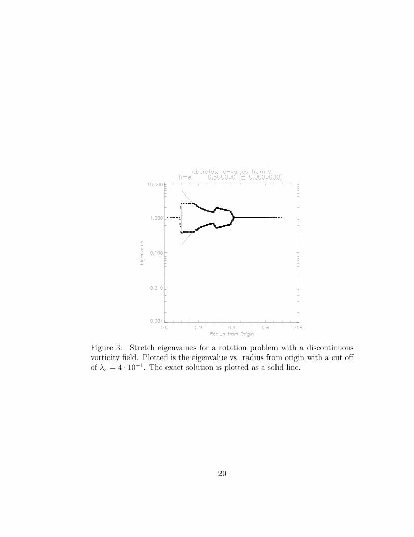
Figure 3: Stretch eigenvalues for a rotation problem with a discontinuousvorticity field. Plotted is the eigenvalue vs. radius from origin with a cut offof λs = 4 · 10−1. The exact solution is plotted as a solid line.
20
where
a =√
(R11 + R22)2 + (R21 − R12)2 (2.32)
Expanding the terms inside the radical shows that
a =√
R211 + R2
12 + R221 + R2
22 + 2 det R (2.33)
and since the remapped rotation matrices should be close to proper orthog-onal rotation matrices over one remap step it is clear that a should notapproach zero and the algorithm should be well defined and robust.
In three dimensions we have used both a direct method provided byScherzinger25 and an iterative method provided by Brannon.4 Fast meth-ods for polar decompositions of non-singular matrices have been studied indetail.12,13,15 Brannon’s algorithm extracts the rotation part of R via a fixedpoint iteration, which converges if the maximumal eigenvalue of R is less than√
3. Since the orthonormal part of a tensor is invariant to scalar multiples,first rescale R according to
R0 =
√
3
tr(RT R)R. (2.34)
If λ21 ≤ λ2
2 ≤ λ23 are the non-zero ordered eigenvalues of (R0)TR0, then by
construction λ21 + λ2
2 + λ23 = 3 and λ2
3 < 3. Thus, iterating
Rm+1 =1
2Rm[3I − (Rm)TRm]. (2.35)
is guaranteed to converge to the nearest orthonormal tensor. The iterationstops for some M where ||(RM)T (RM) − I||2 < ε2 and ε is an small numberclose to machine precision and then R is set to RM . The componentwiseremap generally produces updated rotation tensors, R that are “nearly” or-thonormal, and the iterative projection method usually converges to machineprecision in just a few iterations to produce an orthonormal R.
21

3 Quaternion Representation VR Method (QVR)
A more compact representation for a rotation is available in terms of quate-rions.1,38 Quaternions form an algebra called a division ring in which the ele-ments of the algebra are not commutative under multiplication.11 A quater-nion can be represented as q = (s,v) where s is real and v is a vector. Thequaternion product is given by
q1q2 = (s1,v1)(s2,v2) = (s1s2 − v1 · v2, s1v2 + s2v1 + v1 × v2).
The quaternion inverse is q−1 = q/(qq) with q = (s,−v) and the quaternionnorm is |q| =
√qq.
The space of quaterions with unit magnitude represents rotations throughthe correspondence
q = (cos(θ/2), sin(θ/2)u) = exp((0,ωt/2))
where θ = |ωt| is the rotation angle and u = ω/|ω| is unit spin axis. Theproducts of unit quaterions are also unit quaternions. The mapping to arotation tensor is given by
R = (2s2 − 1)I + 2v ⊗ v + 2sv (3.36)
where v represents the skew-symmetric tensor such that vh = v × h for allh, and v ⊗ v = vivj. Thus the rotation in three dimensions can be thoughtof as being given by a real 4-vector with unit scaling. In two dimensionsonly s and vz are non-zero so the rotation can be represented by a vector oflength two. In both cases we use one more degree of freedom to representthe rotation than strictly required. One way to think of this is that insteadof storing the rotation angle we are storing the sine and the cosine of theangle. Thus when it comes time to obtain a rotation matrix only algebraicoperations are required and no-transcendental functions are needed. We arestill far ahead in term of compactness since 9 and 4 storage locations arerequired in 3D and 2D respectively in the VR case discussed in the previoussection.
The quaternion rotation differential equation is
q = (0,ω/2)q
22

which can be solved exactly for constant axis spin vector ω as an exponentialin the quaternion algebra.
q(t) = exp((0,ω/2)t)q(0) = (cos(|ωt|/2), sin(|ωt|/2)ω
|ω|)q(0).
Thus any constant spin rotation update can be computed exactly with twotranscendental function evaluations and some minor algebra. The majoradvantage of the quaternion representation of a rotation update is that asubsequent rotation can be represented simply as a quaternion product asshown above.
The Lagrangian update algorithm for V is unaffected. The natural La-grangian rotation update algorithm for the quaternion representation is theexponential map,
qn+1 = exp(0,ωn+ 1
2
∆t/2)qn = exp(0,α)qn. (3.37)
We term this Lagrangian algorithm the LQVR algorithm.
It may be useful, in a similar manner to the VR algorithm, to generatethe midstep rotation from the values at the end points. Recall that
qn+1 = (cos(|α|), sin(|α|)α
|α|)qn (3.38)
In order to compute |α| it is easily seen that
qn+1q−1n + qn+1q−1
n
2= sn+1sn + vn+1 · vn = cos(|α|). (3.39)
To compute the rotation at the half step some algebra shows that
exp(0,α/2) = (cos(|α/2|), sin(|α/2|)α
|α|) =
1
2 cos(|α/2|)((1,0) + exp(0,α))
(3.40)and therefore
qn+1/2 = exp(0,α/2)qn =1
2 cos(|α/2|)(qn+1 + qn) (3.41)
23
3.1 QVR Remap
In this representation we remap the components of V exactly as in the VRcase. However, the rotation treatment is vastly different. The conservativeremap algorithm is applied to each component of q so that only 2 componentsin 2D and 4 components in 3D are remapped. Since the remap routine is amajor computational cost we expect significant savings over the VR case.
In addition, the algorithm for keeping the quaternions representation inthe proper space is much simpler when compared to the complex rotationtensor projection methodologies outlined in the previous section. The stan-dard procedure for dealing with floating point roundoff in rotation quaternionupdates is to rescale the quaternion to unit magnitude. In the remap case,truncation error will enter into the quaternion representation of the remappedfield and we will obtain a qr which does not exactly represent a rotation. Wecan however still use the same simple scaling methodology to ensure that thequaternion does indeed represent a rotation. That is, q = qr/
√qrqr.
We tested this algorithm with and without renormalization, and foundthat for particularly severe, discontinuous deformations, renormalization ledto much more accurate results. For smooth problems it made little difference.Because the renormalization is inexpensive, we have used it in all subsequenttests.
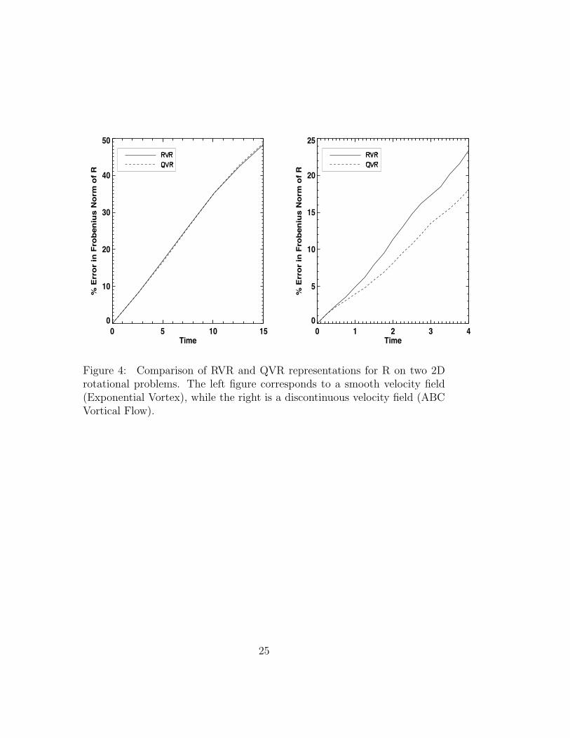
In Figure 4, we compare the results of two two-dimensional rotation prob-lems using the RVR and QVR algorithms. The comparison is based on apercent L2 error norm in R calculated with the equation
√
∑∑
|Rijcalc − Rijexact|2
∑∑
|Rijexact|2
(3.42)
Note that all differences here, up to roundoff errors, are due to the differ-ences between remapping the four-component tensor and the two-componentquaternion and to the differences in renormalization. Time integration doesnot play a factor in the differences seen because the RVR and QVR algo-rithms both use the exponential map instead of the Cayley transformation.Both test problems show that the QVR representation yields equivalent re-sults or better. This seems reasonable because in the quaternion case, theremap step has fewer degrees of freedom.
24
0 5 10 15Time
0
10
20
30
40
50
% E
rror
in F
robe
nius
Nor
m o
f R
0 1 2 3 4Time
0
5
10
15
20
25
% E
rror
in F
robe
nius
Nor
m o
f R
Figure 4: Comparison of RVR and QVR representations for R on two 2Drotational problems. The left figure corresponds to a smooth velocity field(Exponential Vortex), while the right is a discontinuous velocity field (ABCVortical Flow).
25
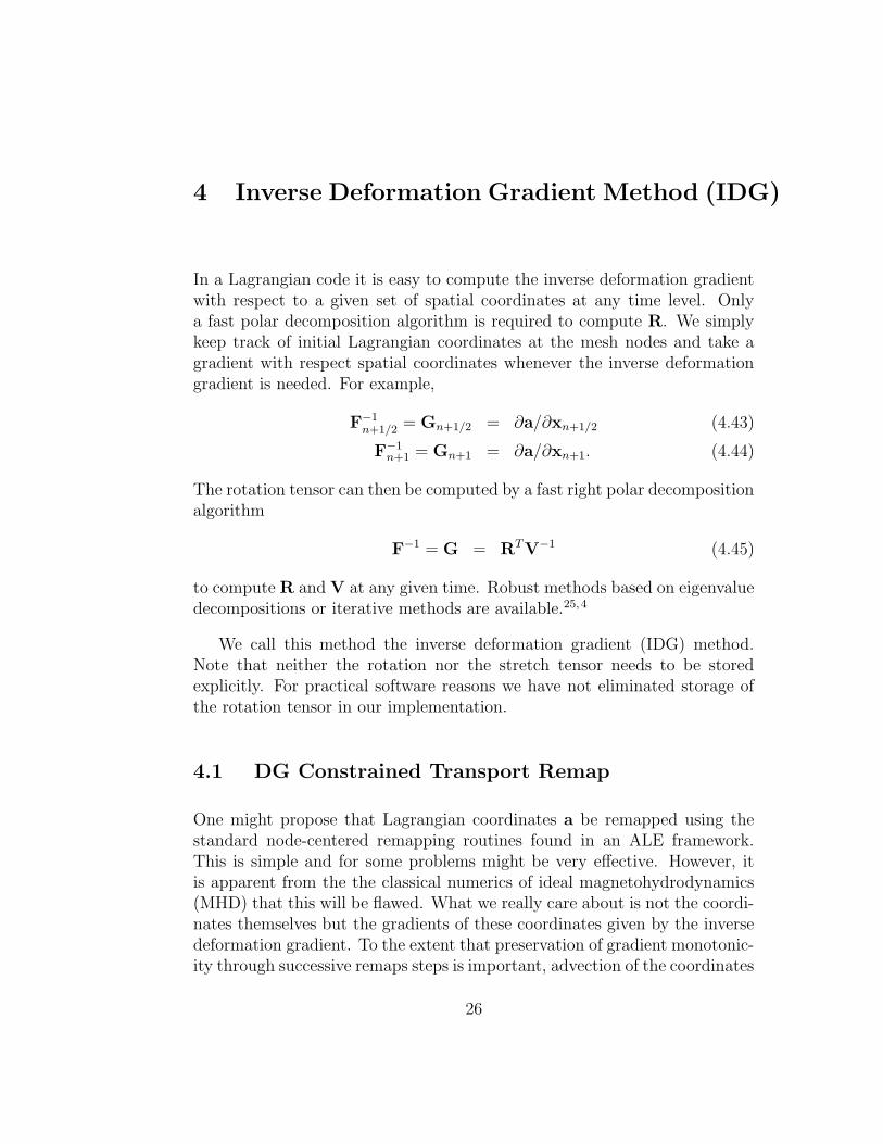
4 Inverse Deformation Gradient Method (IDG)
In a Lagrangian code it is easy to compute the inverse deformation gradientwith respect to a given set of spatial coordinates at any time level. Onlya fast polar decomposition algorithm is required to compute R. We simplykeep track of initial Lagrangian coordinates at the mesh nodes and take agradient with respect spatial coordinates whenever the inverse deformationgradient is needed. For example,
F−1n+1/2
= Gn+1/2 = ∂a/∂xn+1/2 (4.43)
F−1n+1 = Gn+1 = ∂a/∂xn+1. (4.44)
The rotation tensor can then be computed by a fast right polar decompositionalgorithm
F−1 = G = RTV−1 (4.45)
to compute R and V at any given time. Robust methods based on eigenvaluedecompositions or iterative methods are available.25,4
We call this method the inverse deformation gradient (IDG) method.Note that neither the rotation nor the stretch tensor needs to be storedexplicitly. For practical software reasons we have not eliminated storage ofthe rotation tensor in our implementation.
4.1 DG Constrained Transport Remap
One might propose that Lagrangian coordinates a be remapped using thestandard node-centered remapping routines found in an ALE framework.This is simple and for some problems might be very effective. However, itis apparent from the the classical numerics of ideal magnetohydrodynamics(MHD) that this will be flawed. What we really care about is not the coordi-nates themselves but the gradients of these coordinates given by the inversedeformation gradient. To the extent that preservation of gradient monotonic-ity through successive remaps steps is important, advection of the coordinates
26

themselves is a problem. In MHD, non-preservation of monotonicity resultsin highly undesirable and unphysical current reversals. Non-monotonicity ofthe inverse deformation gradient may not be as critical for solid dynamicapplications but may still lead to undesirable solution characteristics or nu-merical breakdown. Fortunately, aspects of this remapping problem havealready been addressed in the MHD community.
The constrained transport (CT) algorithm introduced by Evans and Haw-ley on structured meshes provides a mechanism for advection of magnetic fluxdensity, B, which also exactly preserves a discrete ∇ ·B = 0 property.6 Theconstrained transport algorithm is applicable to a staggered field representa-tion where the magnetic flux is represented on cell faces and the electric fieldson cell edges. In the finite element context the appropriate generalization ofthe CT staggered magnetic field representation is given by edge and facefinite element bases. These bases form a deRham complex for nodes, edges,faces and volumes connected by the operators ∇, ∇× and ∇·, respectivelyin the sense that the gradient of the nodes yields edges, the curl of the edgesyields faces and the divergence of the faces yields volume. It is then naturalto try to extend the CT algorithms to unstructured meshes since the finiteelement formalism of the deRham complex matches precisely the geometryrequired for computing high order upwind fluxes in the structured grid CTalgorithm. A solenoidal field B may be generated from a vector potential Athrough the relationship
B = ∇× A.
A is naturally represented by edge elements with circulations on edges asdegrees of freedom, and B is given by the solenoidal subspace of face ele-ments with fluxes on faces. The degrees of freedom of A and B are relatedby simple algebraic relations in which the fluxes are represented as sums ofcirculations. Londrillo and Del Zanna have noted that the constrained trans-port algorithm is applicable to advection of vector potentials provided thatthe vector potential is properly represented on edges.17 Vector potential for-mulations have been considered to be deficient representations for advectionof magnetic fields due to errors which accumulate during the remap process.This is strictly true only if one insists on remapping nodal vector potentialvalues using some standard reconstruction and limiting procedure for nodalquantities. If the limiting is carried out in the flux density space, good al-gorithms can be obtained. If vector potential components are representedon edges, it is natural to compute edge centered updates in terms of a high
27

order magnetic flux representation. In this case there is no essential differ-ence between a vector potential formulation and a flux centered approachbecause the updates in the first case are added to the vector potential whilethe curl of the updates is added to the face centered fluxes in the second case.Constrained transport succeeds because advection is based on reconstructionand limiting of the underlying field instead of the vector potential. This en-sures that the gradients of the vector potential have monotonic properties.Advecting the vector potential directly can be disastrous because underlyinggradients will not be monotonic and current reversals can be introduced.
Returning now to the kinematics of solids, the basic constrained trans-port ideas for magnetic flux remapping are readily applicable to constrainedtransport for Lagrangian positions or associated gradients. Lagrangian coor-dinates can be considered to be the “potentials” of the inverse deformationgradient fields. The difference now is that we are trying to stay within a“curl free” space so we expect to either update potentials on nodes or up-date circulations on edges as gradients of nodal increments. The idea is toensure that the deformation gradient representation always lives in the curlfree subspace of edge elements. We do this by representing each row g ofG as an edge element. The degrees of freedom on each edge are the circu-lations of the coordinate gradients which are initialized with the point wisesigned difference of the corresponding initial Lagrangian coordinates. Duringthe Lagrangian step these circulation values must be invariant. During theremap we define a high order representation of this field by extending theedge element description to include edge circulation gradients. Given thisnew representation, we compute an upwind nodal flux contribution at eachnode and then take the gradient to update the edge circulations. This ensuresthat the inverse deformation gradients stays within the space of gradients.
We describe now a constrained transport remapping algorithm for hexa-hedral (quadrilateral) grids for a row of the inverse deformation gradient gwhere g is represented by a low order edge element. The algorithm consistsof several parts:
1. Compute the second-order limited reconstruction of the inverse defor-mation gradient field by computing a circulation slope centered on eachedge.
28
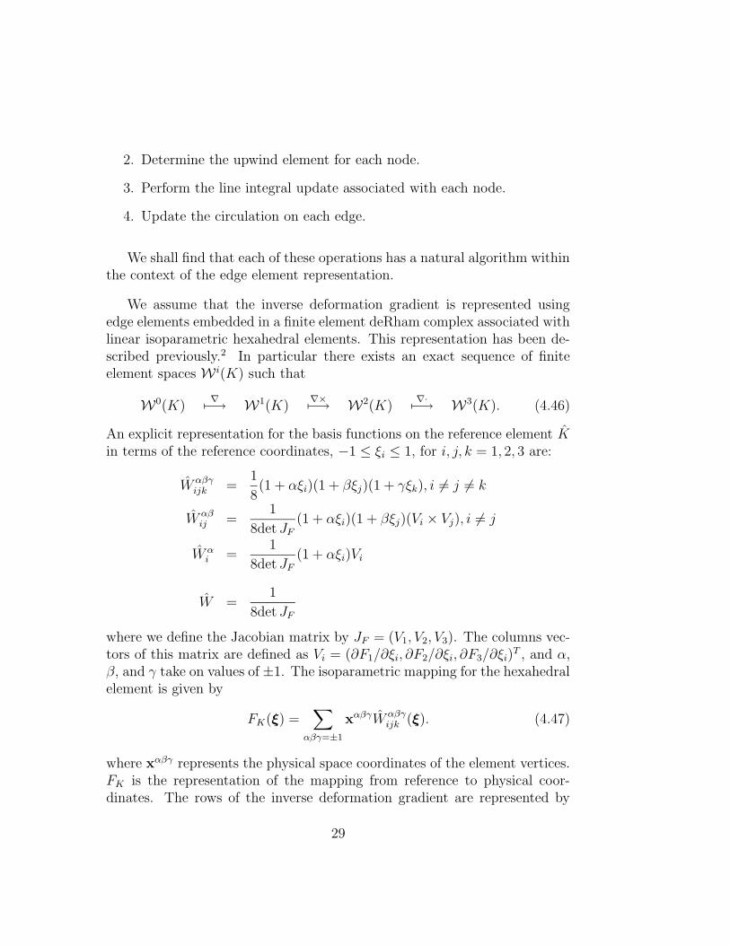
2. Determine the upwind element for each node.
3. Perform the line integral update associated with each node.
4. Update the circulation on each edge.
We shall find that each of these operations has a natural algorithm withinthe context of the edge element representation.
We assume that the inverse deformation gradient is represented usingedge elements embedded in a finite element deRham complex associated withlinear isoparametric hexahedral elements. This representation has been de-scribed previously.2 In particular there exists an exact sequence of finiteelement spaces W i(K) such that
W0(K)∇(−→ W1(K)
∇×(−→ W2(K)∇·(−→ W3(K). (4.46)
An explicit representation for the basis functions on the reference element Kin terms of the reference coordinates, −1 ≤ ξi ≤ 1, for i, j, k = 1, 2, 3 are:
W αβγijk =
1
8(1 + αξi)(1 + βξj)(1 + γξk), i *= j *= k
W αβij =
1
8det JF(1 + αξi)(1 + βξj)(Vi × Vj), i *= j
W αi =
1
8det JF(1 + αξi)Vi
W =1
8det JF
where we define the Jacobian matrix by JF = (V1, V2, V3). The columns vec-tors of this matrix are defined as Vi = (∂F1/∂ξi, ∂F2/∂ξi, ∂F3/∂ξi)T , and α,β, and γ take on values of ±1. The isoparametric mapping for the hexahedralelement is given by
FK(ξ) =∑
αβγ=±1
xαβγW αβγijk (ξ). (4.47)
where xαβγ represents the physical space coordinates of the element vertices.FK is the representation of the mapping from reference to physical coor-dinates. The rows of the inverse deformation gradient are represented by
29

g(ξ1, ξ2, ξ3) =∑
i&=j,α,β
Γαβij W αβ
ij (4.48)
where Γαβij is the total circulation along each edge. This circulation exactly
equals the discrete difference of the initial Lagrangian coordinate. Elementswhich share an edge also share the properly signed circulation value.
It is necessary to generate second-order accurate point values of g. Thesevalues will be used to compute the corresponding edge-wise circulation gra-dient. Obtaining these values at the element nodes is a non-trivial questionbecause the edge element representation is discontinuous at element nodes. Aprojection operator must be defined to obtain high order accurate estimatesof the field at the nodes. A patch recovery operator is suggested.
The first action in the reconstruction is to extend the definition of theedge element coefficient to contain a linear term proportional to each edge-wise reference coordinate. This term will integrate to zero along the edgethus contributing nothing to the total circulation. However, the term willcontribute to the update integrals associated with each node as describedlater. The edge element representation for each element is now
g(ξ1, ξ2, ξ3) =∑
i&=j &=k,α,β
Γαβij (ξk)W
αβij (4.49)
where, for example,Γαβ
ij (ξk) = Γαβij + sαβ
ij ξk (4.50)
The edge circulation slope values are obtained by limiting based on the nodalreconstructed values in the edge direction. To do so, compute a node centeredcirculation value by dotting the reconstructed g values with the correspond-ing Vk of the attached edge. For example,
g(α,β,±1) · V3(α,β,±1) = Γαβ1,2(±1)/2 (4.51)
where
V3(α,β,±1) =x(α,β, +1) − x(α,β,−1)
2(4.52)
This gives two slopes for each edge.
sαβij (±1) = ±(Γαβ
1,2(±1) − Γαβ1,2) (4.53)
30

and we chose a single slope
sαβij =
0 if sαβij (+1)sαβ
ij (−1) < 0min(sαβ
ij (+1), sαβij (−1)) if sαβ
ij (+1) and sαβij (−1) > 0
max(sαβij (+1), sαβ
ij (−1)) if sαβij (+1) and sαβ
ij (−1) < 0
(4.54)
A basic requirement for computation of the circulation associated witheach node is a knowledge of the upwind element associated with each edge.This is accomplished by computing a node centered position vector offset
−v∆t = δxnc (4.55)
and determining if the direction cosines of the associated elements are positivewith respect to the outward edges. If they are all positive, an offset is presentin that element.
We now need to compute an approximate circulation contribution at eachnode. The line integral at each node is conveniently given in terms of differ-entials in the terms of reference element coordinates ξi.
∫
Γ
g · ds =
∫
Γ
g · (∂x
∂ξ1dξ1 +
∂x
∂ξ2dξ2 +
∂x
∂ξ3dξ3) (4.56)
Since the representation for g is in terms of reference element coordinatesadditional major simplifications will be possible. An appropriate integrationmethod and a domain must be chosen. We chose a one point quadrature rulelocated at the center of the node midpoint offset vector. We define
ξi =δξi
2+ ξnc
i (4.57)
The reference element differentials for the one-point quadrature are dξ1 =δξ1, dξ2 = δξ2 and dξ3 = δξ3. Then
∫
Γ
g · ds ≈ g(ξ) · (∂x
∂ξ1(ξ)δξ1 +
∂x
∂ξ2(ξ)δξ2 +
∂x
∂ξ3(ξ)δξ3) (4.58)
But the reconstructed field is given by Equation 4.49 which leads to∫
Γ
g · ds ≈∑
i&=j &=k,α,β
Γαβij (ξk)W
αβij (ξ)
∂x
∂ξk(ξ)δξk (4.59)
31

which can be simplified to∫
Γ
g · ds ≈∑
i&=j &=k,α,β
Γαβij (ξk)(1 + αξi)(1 + βξj)δξk/8. (4.60)
The update contributions are now available on each node as circulations.These can be added directly to the coordinate (potential) representation onnode or equivalently the gradient of the updates values on each edge can betaken to update the edge circulations.
By construction G must stay within a proper discrete curl free space andwill be acceptable as long as detG > 0. This will be true at the beginningof the calculation but may fail later in the calculation. It is quite unclearwhat a rational fix might be because the degrees of freedom are differences ofLagrangian coordinates on edges. It is possible that an optimization basedremap algorithm similar to the one advocated by Shashkov and Bochev fordivergence free remapping might work.3 We also note that, unlike the VR andQVR update algorithms, the IDG algorithm may not be as easily reduced toan algorithm acting only on regions of space (materials) that require stretchand rotation information. We shall see that these issues along with the costof the current implementation prohibits recommendation of this algorithmat this time for multi-material codes.
32

5 Results for Given 2D Motions
We compare the methods we have described by observing each method’saccuracy and cost. An accurate method converges on smooth solutions atthe expected rate as ∆x is decreased at a fixed Courant number. We expectthat some loss of accuracy will occur for motions that are sufficiently stressful.Cost is represented by the time to solution.
We propose that much can be learned from specific test problems. Thegreatest difficulties are generated by flows with large strains and rotations,and we focus on how fast the stretch, rotation, and/or deformation gradienttensors lose consistency and/or accuracy in various situations. For any giventest, the motion x(a, t) can be specified directly. The deformation gradientis computed directly as a function of the Lagrangian coordinates. To findthe value of the deformation gradient at a spatial point, the motion mustbe inverted before evaluating the deformation gradient. If desired, an alter-native computational method for calculating exact solutions is including inAppendix A.
In each of the following 2D test problems, stretch tensor eigenvalues androtation tensor matrices for both the Lagrangian and ALE cases are com-puted using the following algorithms:
• VR method using the Hughes-Winget algorithm (HWVR)
• VR method using the Rodrigues algorithm (RVR)
• Quaternion representation of the VR method (QVR)
• Inverse Deformation Gradient Method (IDG)
Lagrangian solutions and results are denoted by prepending the letter Lto these acronymns. Computations are repeated on five different squaremeshes, and the convergence rates are calculated. Additionally, the cost ofeach method is compared using the finest grid.
33

5.1 Constant Velocity
We expect all methods to be able to model a constant velocity profile anddeal sensibly with inflow boundary conditions from finite grids. The motionis
x = a + vt (5.61)
with velocityv = v (5.62)
Thus, the exact solution of the deformation gradient is
F = I (5.63)
As expected, all methods yield exact results given these conditions. How-ever, this problem is interesting because it allows us to see a cost comparisonof the simplest of all cases. In Table 1, only slight cost differences are visi-ble between the Lagrangian algorithms. On the other hand, in Table 2, thedirect decomposition algorithm has a visible disadvantage.
Method CPU Time Rel. CPU Time
LHWVR 21.24 1.000
LRVR 22.17 1.044
LQVR 21.50 1.012
LIDG 20.86 0.982
Table 1: Relative and actual CPU time for Lagrangian Constant Velocityproblem
34
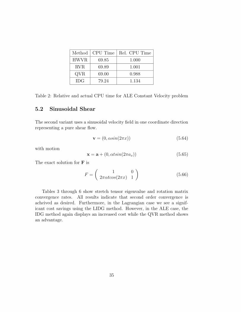
Method CPU Time Rel. CPU Time
HWVR 69.85 1.000
RVR 69.89 1.001
QVR 69.00 0.988
IDG 79.24 1.134
Table 2: Relative and actual CPU time for ALE Constant Velocity problem
5.2 Sinusoidal Shear
The second variant uses a sinusoidal velocity field in one coordinate directionrepresenting a pure shear flow.
v = (0,αsin(2πx)) (5.64)
with motionx = a + (0,αtsin(2πax)) (5.65)
The exact solution for F is
F =
(
1 02παtcos(2πx) 1
)
(5.66)
Tables 3 through 6 show stretch tensor eigenvalue and rotation matrixconvergence rates. All results indicate that second order convergence isacheived as desired. Furthermore, in the Lagrangian case we see a signif-icant cost savings using the LIDG method. However, in the ALE case, theIDG method again displays an increased cost while the QVR method showsan advantage.
35

LHWVR LRVR LQVR LIDG
1/h
16
32
64
96
128
L1 Order
1.07E-01 –
2.70E-02 1.99
6.77E-03 2.00
2.98E-03 2.02
1.67E-03 2.01
L1 Order
1.07E-01 –
2.70E-02 1.99
6.77E-03 2.00
2.98E-03 2.02
1.67E-03 2.01
L1 Order
1.07E-01 –
2.70E-02 1.99
6.77E-03 2.00
2.98E-03 2.02
1.67E-03 2.01
L1 Order
1.03E-01 –
2.57E-02 2.00
6.43E-03 2.00
2.86E-03 2.00
1.61E-03 2.00
Table 3: Stretch tensor eigenvalue convergence rates for Lagrangian Sinu-soidal Shear problem.
LHWVR LRVR LQVR LIDG
1/h
16
32
64
96
128
L1 Order
2.09E-03 –
5.99E-04 1.80
1.51E-04 1.98
6.36E-05 2.14
3.56E-05 2.02
L1 Order
2.00E-03 –
5.61E-04 1.83
1.38E-04 2.02
5.87E-05 2.11
3.28E-05 2.02
L1 Order
2.00E-03 –
5.61E-04 1.83
1.38E-04 2.02
5.87E-05 2.11
3.28E-05 2.02
L1 Order
1.81E-03 –
4.94E-04 1.87
1.16E-04 2.10
5.03E-05 2.05
2.82E-05 2.01
Table 4: Rotation tensor matrix convergence rates for Lagrangian SinusoidalShear problem.
HWVR RVR QVR IDG
1/h
16
32
64
96
128
L1 Order
1.13E-01 –
2.86E-02 1.98
7.17E-03 1.99
3.19E-03 2.00
1.75E-03 2.09
L1 Order
1.13E-01 –
2.86E-02 1.98
7.17E-03 1.99
3.19E-03 2.00
1.75E-03 2.09
L1 Order
1.13E-01 –
2.86E-02 1.98
7.17E-03 1.99
3.19E-03 2.00
1.75E-03 2.09
L1 Order
1.03E-01 –
2.57E-02 2.00
6.43E-03 2.00
2.86E-03 2.00
1.61E-03 2.00
Table 5: Stretch tensor eigenvalue convergence rates for ALE SinusoidalShear problem.
36

HWVR RVR QVR IDG
1/h
16
32
64
96
128
L1 Order
2.44E-03 –
7.07E-04 1.79
1.82E-04 1.96
8.20E-05 1.97
4.10E-05 2.41
L1 Order
2.25E-03 –
6.36E-04 1.82
1.59E-04 2.00
7.11E-05 1.99
3.66E-05 2.31
L1 Order
2.25E-03 –
6.36E-04 1.82
1.59E-04 2.00
7.11E-05 1.99
3.66E-05 2.31
L1 Order
1.81E-03 –
4.94E-04 1.87
1.16E-04 2.10
5.02E-05 2.05
2.82E-05 2.01
Table 6: Rotation tensor matrix convergence rates for ALE Sinusoidal Shearproblem.
Method CPU Time Rel. CPU Time
LHWVR 1641.68 1.000
LRVR 1648.11 1.004
LQVR 1621.37 0.988
LIDG 1448.29 0.882
Table 7: Relative and actual CPU time for Lagrangian Sinusoidal Shearproblem
Method CPU Time Rel. CPU Time
HWVR 462.90 1.000
RVR 460.32 0.994
QVR 459.66 0.993
IDG 556.25 1.202
Table 8: Relative and actual CPU time for ALE Sinusoidal Shear problem
37

5.3 Exponential Vortex
This simple smooth vortical flow asymptotes to an irrotational 1/r angularvelocity profile
vθ =Γ
2πr(1 − e−r2/2) (5.67)
where Γ is the total circulation at infinity. Since the flow is parameterizedby the radius we can compute the motion and thus the deformation gradientexactly. In particular, in polar coordinates
r = r0
θ =Γt
2πr2(1 − e−r2/2) + θ0 (5.68)
and via the chain rule one can compute the deformation gradient in Cartesiancoordinates. The vorticity profile is
ω =1
r
∂
∂r(rvθ) =
Γ
2πe−r2/2 (5.69)
showing that a small cylindrical region of vorticity generates the flow.
As with the Sinusoidal Shear problem, the stretch tensor eigenvalue androtation matrix converges at second-order. The LIDG algorithm again showssome cost benefits in the Lagrangian case, and the QVR method has a slightadvantage in the ALE case.
LHWVR LRVR LQVR LIDG
1/h
16
32
64
96
128
L1 Order
3.93E-02 –
1.03E-02 1.94
2.60E-03 1.98
1.16E-03 1.99
6.52E-04 2.00
L1 Order
3.93E-02 –
1.03E-02 1.94
2.60E-03 1.98
1.16E-03 1.99
6.52E-04 2.00
L1 Order
3.93E-02 –
1.03E-02 1.94
2.60E-03 1.98
1.16E-03 1.99
6.52E-04 2.00
L1 Order
3.95E-02 –
1.03E-02 1.94
2.61E-03 1.98
1.17E-03 1.99
6.56E-04 2.00
Table 9: Stretch tensor eigenvalue convergence rates for Lagrangian Expo-nential Vortex problem.
38

LHWVR LRVR LQVR LIDG
1/h
16
32
64
96
128
L1 Order
9.99E-02 –
2.72E-02 1.87
6.95E-03 1.97
3.10E-03 1.99
1.75E-03 2.00
L1 Order
9.96E-02 –
2.72E-02 1.87
6.93E-03 1.97
3.09E-03 1.99
1.74E-03 2.00
L1 Order
9.96E-02 –
2.72E-02 1.87
6.93E-03 1.97
3.09E-03 1.99
1.74E-03 2.00
L1 Order
9.99E-02 –
2.72E-02 1.87
6.96E-03 1.97
3.10E-03 1.99
1.75E-03 2.00
Table 10: Rotation tensor matrix convergence rates for Lagrangian Expo-nential Vortex problem.
HWVR RVR QVR IDG
1/h
16
32
64
96
128
L1 Order
5.54E-02 –
1.07E-02 2.37
2.01E-03 2.42
7.93E-04 2.30
4.10E-04 2.29
L1 Order
5.54E-02 –
1.07E-02 2.37
2.01E-03 2.42
7.93E-04 2.30
4.10E-04 2.29
L1 Order
5.54E-02 –
1.07E-02 2.37
2.01E-03 2.42
7.93E-04 2.30
4.10E-04 2.29
L1 Order
1.50E-01 –
5.73E-02 1.38
1.67E-02 1.78
7.57E-03 1.95
4.33E-03 1.94
Table 11: Stretch tensor eigenvalue convergence rates for ALE ExponentialVortex problem.
Method CPU Time Rel. CPU Time
LHWVR 116.91 1.000
LRVR 116.98 1.001
LQVR 116.98 1.001
LIDG 103.93 0.889
Table 12: Relative and actual CPU time for Lagrangian Exponential Vortexproblem
39

Method CPU Time Rel. CPU Time
HWVR 184.57 1.000
RVR 182.77 0.990
QVR 179.06 0.970
IDG 187.55 1.016
Table 13: Relative and actual CPU time for ALE Exponential Vortex prob-lem
5.4 Diverging Flow
It is equally important to consider flows with non-trivial volume change. Weconsider flows with constant non-zero divergence in both cylindrical (d = 2)and spherical (d = 3) geometry .
vr = αr/d (5.70)
where α is the divergence which will be recalled represents the logarithmderivative of density. The flow density will change exponentially in time.The general solution is
ρ(r, t) = ρ(re−αt/d, 0)e−αt (5.71)
where ρ(r, 0) is the initial density. In addition, x = aeαt/d so that F = eαt/dIand detF = eαt. This test case is able to discriminate issues related todivergent flow.
Stretch tensor convergence rates are shown in Tables 14 and 15. Rotationtensor convegence rates are not included for this test problem because exactresults were found using every method. In addition, from the tables it canbe seen that the IDG and LIDG methods yield exact results in the stretchtensor while the other methods demonstrate second-order convergence. Thisis expected due to the linear nature of the velocity profile. As for cost, thereseems to be no significant difference between the different methods in theLagrangian case, but IDG continues to exhibit a disadvantage in the ALEcase.
40

LHWVR LRVR LQVR LIDG
1/h
16
32
64
96
128
L1 Order
7.89E-04 –
2.31E-04 1.77
6.29E-05 1.87
2.86E-05 1.94
1.62E-05 1.97
L1 Order
7.89E-04 –
2.31E-04 1.77
6.29E-05 1.87
2.86E-05 1.94
1.62E-05 1.97
L1 Order
7.89E-04 –
2.31E-04 1.77
6.29E-05 1.87
2.86E-05 1.94
1.62E-05 1.97
L1 Order
4.44E-16 –
1.11E-15 NA
2.66E-15 NA
1.56E-14 NA
5.77E-15 NA
Table 14: Stretch tensor eigenvalue convergence rates for Lagrangian Diverg-ing Flow problem.
HWVR RVR QVR IDG
1/h
16
32
64
96
128
L1 Order
2.57E-04 –
7.44E-05 1.79
2.00E-05 1.89
8.58E-06 2.09
4.77E-06 2.04
L1 Order
2.57E-04 –
7.44E-05 1.79
2.00E-05 1.89
8.58E-06 2.09
4.77E-06 2.04
L1 Order
2.57E-04 –
7.44E-05 1.79
2.00E-05 1.89
8.58E-06 2.09
4.77E-06 2.04
L1 Order
2.74E-15 –
3.95E-15 NA
7.28E-15 NA
5.22E-14 NA
1.18E-14 NA
Table 15: Stretch tensor eigenvalue convergence rates for ALE DivergingFlow problem.
Method CPU Time Rel. CPU Time
LHWVR 133.04 1.000
LRVR 133.66 1.005
LQVR 131.84 0.991
LIDG 135.61 1.019
Table 16: Relative and actual CPU time for Lagrangian Diverging Flowproblem
41

Method CPU Time Rel. CPU Time
HWVR 808.47 1.000
RVR 812.77 1.005
QVR 790.02 0.977
IDG 912.10 1.128
Table 17: Relative and actual CPU time for ALE Diverging Flow problem
5.5 ABC Vortical Flow
We now consider a flow field with discontinuities in the vorticity field (i.e.discontinuous velocity gradients). Consider a simple incompressible flow inwhich tangential velocity discontinuities are allowed. A cylindrical block ro-tates at constant angular velocity, surrounded by an irrotational circular flowregion with constant circulation, surrounded finally by a flow with negativevorticity until the flow drops to a zero velocity. The equations for the floware
vθ = ω0r 0 < r < a (5.72)
vθ =ω0a2
ra < r < b (5.73)
vθ =ω0a2
r
(
c2 − r2
c2 − b2
)
b < r < c (5.74)
vθ = 0 c < r (5.75)
This problem provides a region of pure local rotation, a region of pure localstretch, and a mixed region with both stretch and rotation, as well as a qui-escent region. As with the exponential vortex, the solution can be obtainedexplicitly in polar coordinates and the motion and deformation gradient cal-culated explicitly.
Convergence rates for the Lagrangian methods are shown in Tables 18and 19. In this case we get approximately first-order accuracy as might beexpected.
42

LHWVR LRVR LQVR LIDG
1/h
16
32
64
96
128
L1 Order
2.39E-01 –
1.37E-01 0.80
6.03E-02 1.18
3.58E-02 1.29
2.38E-02 1.42
L1 Order
2.39E-01 –
1.37E-01 0.80
6.03E-02 1.18
3.58E-02 1.29
2.38E-02 1.42
L1 Order
2.39E-01 –
1.37E-01 0.80
6.03E-02 1.18
3.58E-02 1.29
2.38E-02 1.42
L1 Order
2.39E-01 –
1.37E-01 0.80
6.03E-02 1.18
3.58E-02 1.29
2.38E-02 1.42
Table 18: Stretch tensor eigenvalue convergence rates for Lagrangian ABCVortical Flow problem.
LHWVR LRVR LQVR LIDG
1/h
16
32
64
96
128
L1 Order
3.93E-01 –
2.80E-01 0.49
1.62E-01 0.79
1.02E-01 1.13
8.17E-02 0.78
L1 Order
3.93E-01 –
2.80E-01 0.49
1.62E-01 0.79
1.02E-01 1.13
8.17E-02 0.78
L1 Order
3.93E-01 –
2.80E-01 0.49
1.62E-01 0.79
1.02E-01 1.13
8.17E-02 0.78
L1 Order
3.93E-01 –
2.80E-01 0.49
1.62E-01 0.79
1.02E-01 1.13
8.17E-02 0.78
Table 19: Rotation tensor matrix convergence rates for Lagrangian ABCVortical Flow problem.
43

Convergence rates for the ALE methods are shown in Tables 20 and 21.It appears that in this ALE case that none of the algorithms are converging.It seems that the gradient jumps in the solution are not well-approximatedand pollute the solution.
HWVR RVR QVR IDG
1/h
16
32
64
96
128
L1 Order
1.77E-01 –
1.24E-01 0.52
7.05E-02 0.81
5.01E-02 0.84
3.83E-02 0.94
L1 Order
1.77E-01 –
1.24E-01 0.52
7.05E-02 0.81
5.01E-02 0.84
3.83E-02 0.94
L1 Order
1.77E-01 –
1.24E-01 0.52
7.05E-02 0.81
5.01E-02 0.84
3.83E-02 0.94
L1 Order
2.58E-01 –
1.81E-01 0.51
1.16E-01 0.64
8.73E-02 0.70
7.14E-02 0.70
Table 20: Stretch tensor eigenvalue convergence rates for ALE ABC VorticalFlow problem.
HWVR RVR QVR IDG
1/h
16
32
64
96
128
L1 Order
3.76E-01 –
1.49E-01 1.34
9.97E-02 0.58
8.66E-02 0.35
8.43E-02 0.09
L1 Order
3.76E-01 –
1.49E-01 1.34
9.96E-02 0.58
8.66E-02 0.35
8.43E-02 0.09
L1 Order
3.70E-01 –
1.42E-01 1.39
9.32E-02 0.60
8.19E-02 0.32
8.05E-02 0.06
L1 Order
4.46E-01 –
2.29E-01 0.96
1.58E-01 0.53
1.36E-01 0.37
1.32E-01 0.10
Table 21: Rotation tensor matrix convergence rates for ALE ABC VorticalFlow problem.
44
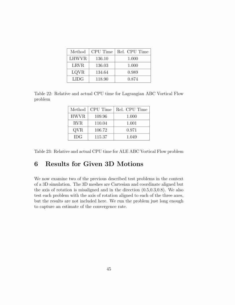
Method CPU Time Rel. CPU Time
LHWVR 136.10 1.000
LRVR 136.03 1.000
LQVR 134.64 0.989
LIDG 118.90 0.874
Table 22: Relative and actual CPU time for Lagrangian ABC Vortical Flowproblem
Method CPU Time Rel. CPU Time
HWVR 109.96 1.000
RVR 110.04 1.001
QVR 106.72 0.971
IDG 115.37 1.049
Table 23: Relative and actual CPU time for ALE ABC Vortical Flow problem
6 Results for Given 3D Motions
We now examine two of the previous described test problems in the contextof a 3D simulation. The 3D meshes are Cartesian and coordinate aligned butthe axis of rotation is misaligned and in the direction (0.5,0.3,0.8). We alsotest each problem with the axis of rotation aligned to each of the three axes,but the results are not included here. We run the problem just long enoughto capture an estimate of the convergence rate.
45

6.1 3D Exponential Vortex
From Tables 24 to 27 it is apparent that second-order convergence is alsoachieved in the 3D version of the Exponential Vortex problem. Additionally,it can be seen that the LIDG algorithm has a large cost advantantage in theLagrangian case, and the QVR algorithm is the fastest in the ALE case.
LHWVR LRVR LQVR LIDG
1/h
4
8
16
32
64
L1 Order
1.58E-01 –
8.12E-02 0.96
2.55E-02 1.67
6.88E-03 1.89
1.75E-03 1.98
L1 Order
1.58E-01 –
8.12E-02 0.96
2.55E-02 1.67
6.88E-03 1.89
1.75E-03 1.98
L1 Order
1.58E-01 –
8.12E-02 0.96
2.55E-02 1.67
6.88E-03 1.89
1.75E-03 1.98
L1 Order
1.58E-01 –
8.12E-02 0.96
2.52E-02 1.69
6.75E-03 1.90
1.71E-03 1.98
Table 24: Stretch tensor eigenvalue convergence rates for 3D LagrangianExponential Vortex problem.
HWVR RVR QVR IDG
1/h
4
8
16
32
64
L1 Order
1.82E-01 –
1.05E-01 0.80
2.93E-02 1.84
6.15E-03 2.25
1.24E-03 2.31
L1 Order
1.82E-01 –
1.05E-01 0.80
2.93E-02 1.84
6.15E-03 2.25
1.24E-03 2.31
L1 Order
1.82E-01 –
1.05E-01 0.80
2.93E-02 1.84
6.15E-03 2.25
1.24E-03 2.31
L1 Order
1.85E-01 –
1.27E-01 0.55
6.65E-02 0.93
2.91E-02 1.19
8.58E-03 1.76
Table 25: Stretch tensor eigenvalue convergence rates for 3D ALE Exponen-tial Vortex problem.
.
46

LHWVR LRVR LQVR LIDG
1/h
4
8
16
32
64
L1 Order
3.16E-01 –
1.26E-01 1.32
3.64E-02 1.79
9.40E-03 1.95
2.37E-03 1.99
L1 Order
3.16E-01 –
1.26E-01 1.32
3.64E-02 1.79
9.40E-03 1.95
2.37E-03 1.99
L1 Order
3.16E-01 –
1.26E-01 1.33
3.62E-02 1.80
9.32E-03 1.96
2.34E-03 1.99
L1 Order
3.17E-01 –
1.28E-01 1.31
3.68E-02 1.79
9.51E-03 1.95
2.39E-03 1.99
Table 26: Rotation tensor matrix convergence rates for 3D Lagrangian Ex-ponential Vortex problem.
HWVR RVR QVR IDG
1/h
4
8
16
32
64
L1 Order
3.47E-01 –
1.76E-01 0.98
5.87E-02 1.58
1.36E-02 2.11
2.93E-03 2.21
L1 Order
3.47E-01 –
1.75E-01 0.98
5.84E-02 1.59
1.34E-02 2.12
2.89E-03 2.22
L1 Order
3.48E-01 –
1.72E-01 1.02
5.33E-02 1.69
1.22E-02 2.13
2.71E-03 2.17
L1 Order
3.92E-01 –
2.62E-01 0.58
1.30E-01 1.01
4.58E-02 1.51
1.32E-02 1.79
Table 27: Rotation tensor matrix convergence rates for 3D ALE ExponentialVortex problem.
Method CPU Time Rel. CPU Time
LHWVR 1870.25 1.000
LRVR 1870.97 1.000
LQVR 1871.89 1.001
LIDG 1693.54 0.906
Table 28: Relative and actual CPU time for 3D Lagrangian ExponentialVortex problem
47

Method CPU Time Rel. CPU Time
HWVR 4220.42 1.000
RVR 4219.98 1.000
QVR 4024.52 0.954
IDG 4364.78 1.034
Table 29: Relative and actual CPU time for 3D ALE Exponential Vortexproblem
6.2 3D ABC Vortical Flow
It will be seen that convergence rates for this problem appear to be ap-proaching first-order for the Lagrangian cases. Something clearly less thanfirst order is in evidence for the ALE results. This is consistent with thenon-smooth nature of the imposed motion.
LHWVR LRVR LQVR LIDG
1/h
4
8
16
32
64
L1 Order
7.76E-02 –
5.99E-02 0.37
2.90E-02 1.05
1.50E-02 0.95
7.19E-03 1.06
L1 Order
7.76E-02 –
5.99E-02 0.37
2.90E-02 1.05
1.50E-02 0.95
7.19E-03 1.06
L1 Order
7.76E-02 –
5.99E-02 0.37
2.90E-02 1.05
1.50E-02 0.95
7.19E-03 1.06
L1 Order
7.77E-02 –
5.99E-02 0.38
2.90E-02 1.05
1.50E-02 0.95
7.20E-03 1.06
Table 30: Stretch tensor eigenvalue convergence rates for 3D LagrangianABC Vortical Flow problem.
48

HWVR RVR QVR IDG
1/h
4
8
16
32
64
L1 Order
7.75E-02 –
6.11E-02 0.34
3.06E-02 1.00
1.68E-02 0.86
8.78E-03 0.94
L1 Order
7.75E-02 –
6.11E-02 0.34
3.06E-02 1.00
1.68E-02 0.86
8.78E-03 0.94
L1 Order
7.75E-02 –
6.11E-02 0.34
3.06E-02 1.00
1.68E-02 0.86
8.78E-03 0.94
L1 Order
7.89E-02 –
6.19E-02 0.35
3.26E-02 0.93
1.90E-02 0.78
1.09E-02 0.81
Table 31: Stretch tensor eigenvalue convergence rates for 3D ALE ABCVortical Flow problem.
LHWVR LRVR LQVR LIDG
1/h
4
8
16
32
64
L1 Order
1.39E-01 –
6.83E-02 1.02
5.19E-02 0.40
3.56E-02 0.54
2.46E-02 0.54
L1 Order
1.39E-01 –
6.83E-02 1.02
5.19E-02 0.40
3.56E-02 0.54
2.46E-02 0.54
L1 Order
1.39E-01 –
6.83E-02 1.02
5.19E-02 0.40
3.56E-02 0.54
2.46E-02 0.54
L1 Order
1.39E-01 –
6.83E-02 1.02
5.19E-02 0.40
3.56E-02 0.54
2.46E-02 0.54
Table 32: Rotation tensor matrix convergence rates for 3D Lagrangian ABCVortical Flow problem.
HWVR RVR QVR IDG
1/h
4
8
16
32
64
L1 Order
1.39E-01 –
6.93E-02 1.00
5.31E-02 0.39
3.66E-02 0.53
2.64E-02 0.47
L1 Order
1.39E-01 –
6.93E-02 1.00
5.31E-02 0.39
3.66E-02 0.53
2.64E-02 0.47
L1 Order
1.39E-01 –
6.93E-02 1.00
5.30E-02 0.39
3.66E-02 0.53
2.64E-02 0.47
L1 Order
1.41E-01 –
7.18E-02 0.97
5.64E-02 0.35
4.05E-02 0.48
3.07E-02 0.40
Table 33: Rotation tensor matrix convergence rates for 3D ALE ABC VorticalFlow problem.
49

Method CPU Time Rel. CPU Time
LHWVR 1149.51 1.000
LRVR 1143.12 0.994
LQVR 1150.23 1.001
LIDG 1049.94 0.913
Table 34: Relative and actual CPU time for 3D Lagrangian ABC VorticalFlow problem
Method CPU Time Rel. CPU Time
HWVR 2459.75 1.000
RVR 2460.67 1.000
QVR 2400.43 0.976
IDG 2668.27 1.085
Table 35: Relative and actual CPU time for 3D ALE ABC Vortical Flowproblem
50

7 A Three Dimensional Impact Problem
Next we compare these various approaches on a more realistic 3D calcula-tion involving the impact of a penetrator into a target. Due to the natureof the problem, only the ALE case is studied. Lagrangian methods do notprove to be sufficiently robust. Furthermore, we do not show the constrainedtransport approach (IDG) because it is not fully implemented and work-ing for multiple material calculations and we have not resolved the issue ofmaintaining positivity of the inverse deformation gradient. Since the currentsingle material implementation is significantly more expensive this algorithmhas not been pursued further.
Table 36 shows time comparisons for the HWVR, RVR, and QVR ap-proaches. In addition, first-order and second-order time stepping schemeshave been implemented with each approach and the two methods that uti-lize a tensor rotation representation (HWVR and RVR) both show resultswith the iterative polar decomposition (Iterative) and the direct polar de-composition (Direct) methods for computating an updated rotation tensorafter component by component remap.
Method Rotation VR Update Time(s) Relative Steps µs/el/stepProjection Time Order Time
HWVR Iterative 1st 166.82 1.0 446 36.528HWVR Iterative 2nd 170.05 1.019 456 36.418HWVR Direct 1st 166.78 1.0 446 36.518HWVR Direct 2nd 171.49 1.028 456 36.726RVR Iterative 1st 167.29 1.003 447 36.547RVR Iterative 2nd 167.28 1.003 447 36.545RVR Direct 1st 166.08 0.996 447 36.284RVR Direct 2nd 171.87 1.03 459 36.567QVR UQuat 1st 172.02 1.031 465 36.127QVR UQuat 2nd 170.76 1.024 459 36.331
Table 36: 3D impact test with varying update methods and representationsfor λs = 10−5.
We observe from this table that using a quaternion representation for
51

the rotation tensor yields a slight computational advantage in terms of com-putational cost per cycle. The extra cost for using the second-order timeintegration VR methodology is barely visible. However, for some reason inthis test case we observe additional cycles indicating some sort of feedbackwhich has lowered the time step for this test problem which leads to no realnet benefit.
We can also optionally compute the midstep rotation tensor using the ex-ponential map interpolation methodology outlined in this report for purposesof allowing hypo-elastic models to be second-order in time. The possibilitywas mentioned in a previous report.7 However, we will not investigate theutility of this approach here as it is intimately involved with the time accu-racy of general non-linear elastic-plastic hypo-elastic models and this subjectdeserves separate attention.26
8 Conclusions
We have characterized various approaches for tracking information associ-ated with the kinematics of the deformation of solid materials when explicitrotation tensors are required. These approaches are applicable for use inLagrangian/Eulerian approaches in which a full kinematic description is re-quired. Examination of the various methods shows that the updated stretchand rotation method with a quaternion representation for the rotation ap-pears to have the advantage at this time. Direct polar decomposition ap-proaches with constrained transport remapping appear to be viable in prin-ciple but the current implementation is not competitive with the updatedpolar decomposition approaches since issues with efficiency, multi-materialmanagement and maintenance of the positivity of the inverse deformationgradient have not yet been resolved.
52

References
[1] David Baraff. An introduction to physically based modeling: Rigidbody simulation I and II. Online Siggraph ’97 Course Notes.http://www.cs.brown.edu/courses/cs224/papers/baraff97notes1.pdf,1997.
[2] P. B. Bochev, J. J. Hu, A. C. Robinson, and R. S. Tuminaro. Towardsrobust 3D Z-pinch simulations: discretization and fast solvers for mag-netic diffusion in heterogeneous conductors. Electronic Transactions onNumerical Analysis, 15:186–210, 2003.
[3] Pavel Bochev and Mikhail Shashkov. Constrained interpolation (remap)of divergence-free fields. Computer Methods Appl. Mech. Engrg.,194:511–530, 2005.
[4] R. M. Brannon. Rotation: A review of useful theoremsinvolving proper orthogonal marices referenced to three-dimensional physical space. Unpublished document available athttp://www.mech.utah.edu/brannon/gobag.html, February 2009.
[5] J. K. Dienes. On the analysis of rotation and stress rate in deformingbodies. Acta Mechanica, 32:217–232, 1979.
[6] Charles R. Evans and John F. Hawley. Simulation of magnetohydrody-namic flows: a constrained transport method. The Astrophysical Jour-nal, 332:659–677, September 1988.
[7] Grant V. Farnsworth and Allen C. Robinson. Improved kinematic op-tions in ALEGRA. Technical Report SAND2003-4510, Sandia NationalLaboratories, Albuquerque, New Mexico, December 2003.
[8] D. P. Flanagan and L. M. Taylor. An accurate numerical algorithm forstress integration with finite rotations. Computer Methods in AppliedMechanical Engineering, 62:305–320, 1987.
[9] J. N. Franklin. Matrix Theory. Prentice-Hall, 1968.
[10] James G. Glimm, Bradley J. Plohr, and David H. Sharp. A conservativeformulation for large-deformation plasticity. Applied Mech. Rev., 46:519–526, 1993.
53
[11] I. N. Herstein. Topics in Algebra. John Wiley & Sons, New York, 1975.
[12] Nicholas J. Higham. Computing the polar decomposition - with appli-cations. SIAM Journal Scientific and Statistical Computing, 7(4):1160–1174, October 1986.
[13] Nicholas J. Higham and Robert S. Schreiber. Fast polar decomposition ofan arbitrary matrix. SIAM Journal Scientific and Statistical Computing,11(4):648–655, July 1990.
[14] Thomas J. R. Hughes and James Winget. Finite rotation effects innumerical integration of rate constitutuve equations arising in large-deformation analysis. Computer Methods in Applied Mechanical Engi-neering, 15(12):1862–1867, 1980.
[15] Charles Kenney and Alan J. Laub. On scaling Newton’s method for po-lar decompositions and the matrix sign function. SIAM Journal MatrixAnalysis, 13(3):688–706, July 1992.
[16] X. Lin and J. Ballmann. A Riemann solver and a second-order Go-dunov method for elastic-plastic wave propagation in solids. Interna-tional Journal of Impact Engineering, 13(3):463–478, 1993.
[17] P. Londrillo and L. Del Zanna. High order upwind schemes for multidi-mensional magnetohydrodynamics. The Astrophysical Journal, 530:508–524, 2000.
[18] G. H. Miller and P. Colella. A high-order Eulerian Godunov method forelastic-plastic flow in solids. Journal of Computational Physics, 167:131–176, 2001.
[19] G. H. Miller and P. Colella. A conservative three-dimensional Eulerianmethod for coupled solid-fluid shock capturing. Journal of Computa-tional Physics, 183:26–82, 2002.
[20] James S. Peery and Daniel E. Carroll. Multi-material ALE methodsin unstructured grids. Computer Methods in Applied Mechanics andEngineering, 187:591–619, 2000.
[21] Bradley J. Plohr. Mathematical modeling of plasticity in metals. Mat.Contemp., 11:95–120, 1996.
54
[22] Bradley J. Plohr and David H. Sharp. A conservative Eulerian formula-tion of the equations for elastic flow. Advances in Applied Mathematics,9:481–499, 1988.
[23] Bradley J. Plohr and David H. Sharp. A conservative formulation forplasticity. Advances in Applied Mathematics, 13:462–493, 1992.
[24] M. M. Rashid. Material state remapping in computational solid me-chanics. International Journal for Numerical Methods in Engineering,55:431–450, 2002.
[25] William M. Scherzinger and Clark R. Dohrmann. A robust algorithmfor finding the eigenvalues and eigenvectors of 3x3 symmetric matrices.Computer Methods in Applied Mechanics and Engineering, 197:4007–4015, 2008.
[26] J. C. Simo and S. Govindjee. Non-linear b-stability and symmetry pre-serving return mapping algorithms for plasticity and viscoplasticity. In-ternational Journal for Numerical Methods in Engineering, 31:151–176,1991.
[27] J. C. Simo and T. J. R. Hughes. Computational Inelasticity. Springer-Verlag New York, Inc., 1998.
[28] J. C. Simo and K. S. Pister. Remarks on rate constitutive equations forfinite deformation problems: Computational implications. ComputerMethods in Applied Mechanics and Engineering, 46:201–215, 1984.
[29] John A. Trangenstein. Adaptive mesh refinement for wave propagationin nonlinear solids. SIAM Journal Scientific Computing, 16(4):819–839,July 1995.
[30] John A. Trangenstein and Phillip Colella. A higher-order Godunovmethod for modeling finite deformation in elastic-plastic solids. Com-munications on Pure and Applied Mathematics, 44:41–100, 1991.
[31] John A. Trangenstein and Richard B. Pember. The Riemann problemfor longitudinal motion in an elastic-plastic bar. SIAM Journal Scientificand Statistical Computing, 12(1):180–207, 1991.
55

[32] John A. Trangenstein and Richard B. Pember. Numerical algorithms forstrong discontinuities in elastic-plastic solids. Journal ComputationalPhysics, 103:63, 1992.
[33] H. S. Udaykumar, L. Tran, D. M. Belk, and K. J. Vanden. An Eule-rian method for computation of multimaterial impact with ENO shock-capturing and sharp interfaces. Journal of Computational Physics,186:136–177, 2003.
[34] John Walter, James Glimm, John Grove, Hyun-Cheol Hwang, Xiao Lin,Brakely J. Plohr, David H. Sharp, and Dahi Yu. Eulerian front trackingfor solid dynamics. In K. Iyer and S. Chou, editors, Proc. 15th U. S.Army Symposium on Solid Mechanics, pages 343–366. Battelle Press,1999.
[35] John Walter, Dahai Yu, Bradley J. Plohr, John Grove, and JamesGlimm. An algorithm for Eulerian front tracking for solid deforma-tion. Technical Report SUNY SB-AMS-00-24, State University of NewYork, 2000.
[36] Feng Wang, James Glimm, and Bradley J. Plohr. A model for rate-dependent plasticity. J. Mech. Phys. Solids, 43(9):1497–1503, 1995.
[37] Feng Wang, James G. Glimm, John W. Grove, Bradley J. Plohr, andDavid H. Sharp. A conservative Eulerian numerical scheme for elasto-plasticity and application to plate impact problems. Impact Computer.Sci. Engrg., 5:285–308, 1993.
[38] Eric W. Weisstein. Quaternion. From MathWorld–A Wolfram WebResource. http://mathworld.wolfram.com/Quaternion.html, 1999 CRCPress LLC, 1999-2004 Wolfram Research, Inc.
56

A Alternative Method For Calculating ExactSolutions
It is possible to compute an arbitrary motion and the associated deformationgradient associated with the specification of a given velocity field, v(x, t).This problem can be solved in general by integrating the set of ordinarydifferential equations (ODE)
x = v(x, t) (A.76)
F = L(x, t)F (A.77)
x(0) = a (A.78)
F(0) = I (A.79)
for any initial Lagrangian position a and L = ∇v. If this set of ODEs can besolved exactly, F(x, t) can be written explicitly which in general is preferable.
If the solution cannot be obtained exactly, it may be obtained numericallyusing an ODE solver as follows. Assume we desire the solution at a point xat times 0 = T0 < T1 < · · · < Tn. We apply a Newton iteration on a for agiven x using
ak+1n = ak
n − F−1(akn)(x(ak
n) − x), k = 0, 1, · · · ,Kn (A.80)
where F and x are obtained by numerical solution of Equations A.76 to A.79to time Tn. The subscript refers to the time level and the superscript to theiteration level. Kn is the number of iterations to achieve convergence. The T0
solution is, of course, ak0 = x, and thereafter we use as initial guesses for the
Newton iteration a0n = aKn−1
n−1 This procedure may be used to compute the“exact” solution corresponding to any desired spatial velocity field providedthat sufficient accuracy is imposed on the ODE solver.
57

DISTRIBUTION:
2 Lawrence Livermore National Lab-oratoryP.O. Box 808Livermore, CA 94551
Attn: D. Bailey, MS L-016Attn: R. N. Rieben, MS L-095
2 Los Alamos National LaboratoryLos Alamos, NM 87545
Attn: M. Shashkov, T-5, MS-B284
Attn: J. Kamm, X-3, MS-B259
1 Air Force Research LaboratoryAFRL/RDHP3550 Aberdeen Ave SE, Bldg 322Kirtland AFB, NM 87117-5776
Attn: D. J Amdahl
3 U.S. Army Research LaboratoryAMSRL-WT-TAAberdeen Proving Ground, MD,21005-5066
Attn: R. DoneyAttn: B. LeavyAttn: M. Love
1 R. M BrannonDepartment of Mechanical Engi-neeringUniversity of Utah50 S. Central Campus Dr.Salt Lake City, UT 84112
1 M. A. ChristonDassult Systemes Simulia Corp.Rising Sun Mills166 Valley StreetProvidence, RI 02909-2499
1 G. H. MillerApplied Science1033 Academic SurgeDavis, CA 95616
1 G. Farnsworth800 Sherman Ave. Apt 2Evanston, IL 60202
1 D. I. KetchesonDepartment of Applied Mathemat-icsUniversity of WashingtonBox 35240 Seattle, WA 98195-2420
1 MS 0316C. C. Ober, 1433
1 MS 0370T. G. Trucano, 1411
1 MS 0372A. S. Gullerud, 1524
1 MS 0372S. T. Montgomery, 1524
1 MS 0372W. M. Scherzinger, 1524
1 MS 0372J. E. Bishop, 1525
1 MS 0378T. L. Ames, 1431
1 MS 0378S. Carroll, 1431
1 MS 0378R. R. Drake, 1431
1 MS 0378D. M. Hensinger, 1431
58

1 MS 0378M. E. Kipp, 1431
1 MS 0378D. A. Labreche, 1431
1 MS 0378E. Love, 1431
1 MS 0378C. B. Luchini, 1431
1 MS 0378S. J. Mosso, 1431
1 MS 0378J. H. Neiderhaus, 1431
1 MS 0378S. V. Petney, 1431
1 MS 0378W. J. Rider, 1431
3 MS 0378A. C. Robinson, 1431
1 MS 0378G. Scovazzi, 1431
1 MS 0378C. Siefert, 1431
1 MS 0378R. M. Summers, 1431
1 MS 0378V. G. Weirs, 1431
1 MS 0378T. E. Voth, 1433
1 MS 0378M. K. Wong, 1431
1 MS 0380N. Crane, 1542
1 MS 0380J. D. Hales, 1542
1 MS 0380M. Heinstein, 1542
1 MS 0380J. Jung, 1542
1 MS 0380K. Pierson, 1542
1 MS 0380B. W. Spencer, 1542
1 MS 0380J. D. Thomas, 1542
1 MS 0382M. W. Glass, 1541
1 MS 0384P. Yarrington, 1550
1 MS 0521K. H. Brown, 2617
1 MS 0836S. C. Schumacher, 1516
1 MS 0836D. A. Crawford, 1541
1 MS 0836R. G. Schmitt, 1541
59

1 MS 0847S. W. Attaway, 1534
1 MS 1189T. A. Brunner, 1641
1 MS 1189S. J. Chantrenne, 1641
1 MS 1189K. R. Cochrane, 1641
1 MS 1189D. G. Flicker, 1641
1 MS 1189C. J. Garasi, 1641
1 MS 1189T. A. Gardiner, 1641
1 MS 1189T. A. Haill, 1641
1 MS 1189H. L. Hanshaw, 1641
1 MS 1189C. S. Kueny, 1641
1 MS 1189R. W. Lemke, 1641
1 MS 1189G. T. Sharp, 1641
1 MS 1189T. K. Mattsson, 1641
1 MS 1189E. P. Yu, 1641
1 MS 1195J. P. Davis, 1646
1 MS 1320P. B. Bochev, 1414
1 MS 1322J. B. Aidun, 1435
1 MS 1322J. H. Carpenter, 1435
1 MS 1323S. Swan, 1431
1 MS 0899Technical Library, 9536
(electronic copy)
60