1

KEY FACTORS FOR CONTROL OF MICRO STEREO LITHOGRAPHY SYSTEM

By

ABHINAV PANDEY

A THESIS PRESENTED TO THE GRADUATE SCHOOL OF THE UNIVERSITY OF FLORIDA IN PARTIAL FULFILLMENT

OF THE REQUIREMENTS FOR THE DEGREE OF MASTER OF SCIENCE

UNIVERSITY OF FLORIDA

2011

2

© 2011 Abhinav Pandey

3

To my family

4

ACKNOWLEDGMENTS

I would like to thank my parents for their continued support and love. I am also

truly grateful to my advisor Prof. Toshikazu Nishida for all his guidance. He supported

me, encouraged me and guided me whenever needed. I feel really fortunate to have

him as my advisor. I have learnt a lot of valuable lessons both academic and

nonacademic, in the past two years while working with him. I believe the experience I

had with him was unique and it will truly help me in my future endeavors and for that I

am really grateful to him. I would also like to thank my friend Raphael. I used to have

really long discussions with him and learnt a lot of valuable stuff. I really enjoyed

working with him and I am thankful to him for all of his support.

5

TABLE OF CONTENTS page

ACKNOWLEDGMENTS .................................................................................................. 4

LIST OF TABLES ............................................................................................................ 6

LIST OF FIGURES .......................................................................................................... 7

LIST OF ABBREVIATIONS ............................................................................................. 8

ABSTRACT ..................................................................................................................... 9

CHAPTER

1 INTRODUCTION .................................................................................................... 10

History ..................................................................................................................... 10

Working Principle .................................................................................................... 11 Issues ..................................................................................................................... 12

2 CURING DEPTH STUDY ....................................................................................... 16

Mathematical Model ................................................................................................ 17 Effect of Absorber Addition ..................................................................................... 20

Effect of Temperature ............................................................................................. 21

Experiment Setup ................................................................................................... 23

3 DIVERGENCE STUDY ........................................................................................... 38

4 CONCLUSION ........................................................................................................ 43

LIST OF REFERENCES ............................................................................................... 45

BIOGRAPHICAL SKETCH ............................................................................................ 47

6

LIST OF TABLES Table page 1-1 Comparison of different micromachining techniques .......................................... 15

3-1 Experimentally computed angle of convergence at different depth .................... 41

7

LIST OF FIGURES

Figure page 1-1 Micro Stereo Lithography system setup ............................................................. 15

2-1 Curing Depth as a function of both initiator and energy dose. ............................ 28

2-2 Curing Depth as a function of time and area of exposure. .................................. 29

2-3 Temperature as a function of time and area of exposure. .................................. 30

2-4 Chemical structure. ............................................................................................. 31

2-5 Experimental setup used for curing depth study. ................................................ 31

2-6 Curing depth as a function of time for constant intensity exposure and absorber concentration of 1%.. ........................................................................... 32

2-7 Curing depth as a function of time for constant intensity exposure and absorber concentration of 3%.. ........................................................................... 33

2-8 Curing depth as a function of time for constant intensity exposure and initiator concentration of 2%.. ............................................................................. 34

2-9 Curing depth as a function of time for constant intensity exposure and initiator concentration of 4%.. ............................................................................. 35

2-10 Curing depth as a function of time for constant intensity exposure. .................... 36

2-11 Result for constant exposure time of 100 sec.. ................................................... 37

2-12 Result for constant curing depth of 100 µm.. ...................................................... 37

3-1 Profile of mask having walls between holes as opaque to UV. ........................... 41

3-2 Diameter of Hole as a function of Depth. ............................................................ 41

3-3 Chemical Structure of SU-8 Photoresist. ............................................................ 41

3-4 Structure developed on SU-8 coated wafer as a function of distance. ............... 42

8

LIST OF ABBREVIATIONS

CAD Computer Aided Design

HDDA Hexanediol Diacrylate

LIGA German acronym for Lithography, Electroplating and Molding

MEMS Micro Electro Mechanical System

µSL Micro Stereo Lithography

ODE Ordinary Differential Equation

Si Silicon

3D Three Dimensional

Ec Threshold Exposure

UV Ultra Violet

3D LCVD 3 Dimensional Laser Chemical Vapor Deposition

9

Abstract of Thesis Presented to the Graduate School of the University of Florida in Partial Fulfillment of the Requirements for the Degree of Master of Science

KEY FACTORS FOR CONTROL OF MICRO STEREO LITHOGRAPHY SYSTEM

By

Abhinav Pandey

May 2011

Chair: Toshikazu Nishida Cochair: David Arnold Major: Electrical and Computer Engineering

Micro stereo lithography (µSL) process is gaining a lot of popularity due to its

ability to fabricate complex and intricate 3D structure over a wide variety of materials. In

order to build a µSL system several parameters need to be known. Some of the most

important parametrs are the curing depth and divergence of light produced by light

source.

Curing depth is calculated as a function of initiator and absorber concentration. An

extensive mathematical model is derived taking into account the initiator concentration,

absorber concentration and temperature effects. Solutions with different absorber and

initiator concentration are used to show the monotonic dependence of initiator and

absorber on curing depth. The exponential dependence of temperature is also

demonstrated.

Divergence study is performed to understand the effects of interference of light

along the edges. As maintaining a closed gap between mask and monomer solution is a

challenge, divergence study is used to derive the maximum allowed separation between

mask and monomer solution.

10

CHAPTER 1 INTRODUCTION

History

A tremendous growth has been observed in the field of micro electro mechanical

system (MEMS) during the past 20 years. Aside from laying planar 2D structure on the

semiconductor substrate, MEMS technologies require micro fabrication of complex 3D

structures. The most typical silicon micro machining technologies, anisotropic etching

and surface micromachining are used in past to produce 3D structures. However, more

complex structures cannot be fabricated using above mentioned techniques. Another

limitation is due to the fact that these processes only apply to a handful of common

semiconductors, metals and dielectrics [1].

In order to have complex 3D structures on a wide variety of materials, Becker et al.

proposed LIGA process in 1986[2]. LIGA is a German word and it stands for

Lithography, Electroplating and Molding. Primary template is formed using lithography

and then its filled by metal using electro deposition. However, very complex structures

cannot be formed using this technique.

3D Laser Chemical Vapor Deposition is presented by Williams and Maxwell [3].

They demonstrated this technology for manufacturing of helical microstructures. 3D

LCVD uses a scanning laser beam to deposit solid materials. The shape of the

fabricated part is controlled by focusing the scanning laser beam.

Another method is proposed by Cohen et al. [4]. They demonstrated

electrochemical fabrication process as an extension of LIGA process to produce

complex 3D structures. Metals are deposited in a layer by layer fashion which acts as

electrode masks. The thickness of the layer is controlled by a planarizing procedure.

11

However, all of the above mentioned techniques suffer from high equipment cost

and a very low throughput.

The shortcomings of the above mentioned techniques are addressed by a new

technique termed stereo lithography. This technique was invented by Chuck Hull in

1986 [5]. This technique forms the basis of micro stereo lithography process. Micro

stereo lithography process is same as stereo lithography process except for the fact that

it is used to make much smaller parts.

Working Principle

The basic idea behind the micro stereo lithography process is the layer by layer

formation of a UV curable resin. Exposing the resin to UV hardens a small layer. This

layer is then moved down and fresh layer of resin covers the hardened surface.

Exposing it again makes the second layer stacked on top of the first one. A schematic of

such a process is shown in Figure 1-1.

Using such a technique, lateral resolution of as low as 600nm is achieved using a

two photon polymerization process [6]. Another important benefit of using micro stereo

lithography is freedom to fabricate on a vast variety of materials. It is not just limited to

UV curable resins. Complex 3D shapes in ceramics and metals also are demonstrated

by mixing fine powder with UV curable resin [7].

Micro stereo lithography can be subdivided into two main sub processes namely

vector by vector micro stereo lithography and integral micro stereo lithography. In vector

by vector approach a focused light beam is scanned on the surface of monomer [8]. It

provides a very high level of resolution. It does not require any mask or any specific

tool. A complex 3D structure with very high aspect ratio can be fabricated by slicing a

12

3D CAD file. However, the process takes a lot of time and thus not suitable for batch

production of micro structures.

On the other hand, in the integral micro stereo lithography a complete layer of

monomer is exposed by projecting the image on it. In order to generate complex

structure a digital micro mirror or an Liquid Crystal Display device can be used to project

the image of cross section [9, 10]. To fabricate simple structure with high aspect ratio a

fixed mask can also be used. The bitmap image is used to pattern light (typically UV)

which is then focused onto the surface of a light curable resin to form a layer.

Subsequent layers are built on top of previous layers to form a 3D structure. Because

the light is focused, the realizable cross sectional is restricted. This limitation to mask

projection micro stereo lithography can be overcome by "stitching" multiple segments of

the total desired cross section together using a stage that can articulate in the X, Y

axes. Multiple overlapping exposures are made at each level thus quilting together the

total desired cross sectional area [11]. A comparison of different micro stereo

lithography technique is shown in Table 1-1.

Issues

One of the main challenges in micro stereo lithography fabrication is to accurately

quantify the curing depth. When a monomer solution is exposed to light, the extent of

polymerization gradually decreases with an increase in depth from the surface. Curing

depth is defined as the depth inside the monomer solution up to which a critical

polymerization is occurred on UV exposure. It is usually a complex function of exposure

dose, reactivity of monomer solution and temperature of the monomer solution. Curing

depth dictates the thickness of layer to be formed. If a particular thickness is required,

the amount of exposure dose needed is also governed by curing depth. Another

13

important issue is the viscosity of the UV curable resin. In layer by layer formation

method after each step a fresh layer of monomer is required on top of polymerized

surface. Also this small layer needs to be flat to ensure uniform polymerization across

the entire cross section. After each step some time is required for fresh monomer layer

to level across the surface. A more viscous liquid will require a longer leveling time and

it may also happen that it will not level at all. In such a case platform should be dipped

inside and then lifted back up [12].

Some other factors that limit the resolution of the micro stereo lithography process

are bleaching and print through. At high exposure doses, stereo lithography monomers

undergo bleaching as the polymerization reactions precede. As a consequence of

bleaching, radiation penetrates the monomer more easily, thus causing polymerization

at greater depths. Increased polymerization depths result in lower Z resolution. This

phenomenon is known as bleaching effect [13]. Another challenge is the print through

error [14]. When a layer is polymerized, the layer thickness is set to the depth where the

exposure falls to the threshold exposure Ec. The monomer below this cured layer does

not experience an exposure equal to Ec. However, it receives some exposure. As

subsequent layers are polymerized, this point in the monomer receives incremental

exposure until finally reaching Ec causing polymerization. The result is unwanted curing

and the error introduced is called the print- through error.

This work deals with the issues mentioned above. An in depth study of curing

depth is performed and presented in Chapter 2. The effect of absorber concentration,

initiator concentration, light intensity and temperature is taken into account. The

mathematical model is also supported by the experimental results.

14

The lateral resolution can also be limited by the divergence of collimated light

source. A diverging light would set a maximum allowable separation between light

source and monomer layer. Chapter 3 addresses the issue of divergence of collimated

light source. Experimental results are shown to quantify the effect upon lateral

resolution as a function of separation between a light source and monomer layer.

Chapter 4 summarizes the results of curing depth study and divergence study.

15

Table 1-1. Comparison of different micromachining techniques

Method Pros Cons

LIGA High resolution High aspect ratio

Used for simpler structure

3D Laser CVD Free standing helical structure

Fast

Limited material process Expensive

EFab True 3D geometry Fast

For metals only Expensive

2 Photon µSL Submicron resolution Layer by layer is not needed Fast build time

Very expensive Limited area of exposure Slow over large area

Vector by Vector µSL High Resolution Fast build time Complex free standing

structure

Limited area of exposure Slow over large area Expensive

Integral µSL Fast over large area High resolution Complex Structure

High cost of equipment Limited area of exposure

Figure 1-1. Micro Stereo Lithography system setup

16

CHAPTER 2 CURING DEPTH STUDY

Curing depth is defined as the depth up to which 3 dimensional gel networks is

formed, when monomer solution is irradiated with light. The critical conversion point of

gel network known as gelation decides the level of polymerization. This conversion point

is a function of both reaction rate and amount of photons present. Active research has

been going on to study the reaction kinetics of these systems [15, 16]. Numerous

parameters influence the polymerization reaction rate. Some of the most influential

parameters are temperature, concentration of absorber and initiator and light intensity.

The effect of these parameters on overall bond conversion is well known however, an in

depth study for the roles of these parameter on cure depth has not been done.

The typical reactants in photo polymerization reaction are initiator, and monomer

molecule. The reaction mainly consists of three steps. The first step is initiation of free

radical by photo radiation. The reaction involved is as follow

→

The initiator molecule is split to generate free radicals when UV light shines upon it

and is denoted by . These free radicals combine with monomer molecules to generate

longer chain radicals or oligomers. This process step is known as propagation and the

reactions involved are as follows

→

→

The last step is the termination. Free radicals can combine with it or can combine

with a chain to terminate the reaction. The reactions involved are as follows

[2-1]

[2-2]

[2-3]

17

→

→

→

Mathematical Model

A model for curing depth is derived using the kinetic equation for photoinitiated

polymerization [17].

[ ]

where is given by

[ ][ ]

is the rate of polymerization and is the rate of initiation of free radical by UV

light exposure. [ ] is the concentration of monomer and [ ] is the concentration of

radical chain. is the reaction rate constant of propagation. During steady state,

initiation of radicals due to light impingement is balanced by termination. Hence using

the steady state approximation, [ ] can be expressed [17].

[ ]√

where is the rate of initiation of polymer and is the reaction rate constant of

termination. The initiation rate is a function of intensity of incident light. Its value is

given by

[ ]

is the intensity of light at a depth z in the monomer solution. [ ] is the

concentration of initiator, is the quantum yield of photo initiator and is the molar

[2-4]

[2-5]

[2-6]

[2-7]

[2-8]

[2-9]

[2-10]

18

extinction coefficient. Intensity of incident light at depth z can be given by Beer Lambert

law. As the monomer solution is homogenous and scattering of light is negligible, Beer

Lambert law can be applied. According to this, intensity of light in a medium at a depth z

is given by [18, 19]

[ ]

where is the intensity of light at the surface. Hence Equation 2-10 can be written

as

[ ] [ ]

Substituting the value of in the Equation 2- 12

[ ]

[ ]√

[ ] [ ]

Assuming the terms on right hand side are time independent, separation of

variable can be used to obtain a closed form solution of the differential equation.

However, if the temperature dependence of reaction rate constant and are taken

into account, no closed form solution can be obtained. Thus the temperature

dependence is handled later in this chapter and numerical solutions are generated

using MATLAB®.

Bringing [ ] on the left hand side and integrating with respect to time yields

([ ]

[ ]) ( √

[ ] [ ]

)

The degree of polymerization is defined as

[ ] [ ]

[2-11]

[2-12]

[2-13]

[2-14]

[2-15]

19

The relationship between degree of polymerization and extent of polymerization

p can be given as

Substituting this and squaring both sides yield

( ( ))

[ ]

[ ]

Curing depth is defined as the depth at which the extent of polymerization reaches

a threshold known as gel point [20, 21]. At this threshold transition from polymer to

monomer takes place and it limits the curing depth. Substituting this and taking natural

log on both sides

[ ] (

( )√

[ ]

)

Equation 2-18 reveals the dependence of curing depth on exposure time t and

initiator concentration [ ]. As initiator concentration is increased, the rate of reaction

increases, however, the increase in initiator concentration decreases the amount of

photon reached at depth z. These two conflicting behaviors give rise to an optimal value

of initiator concentration beyond which curing depth starts to decrease. Differentiating

with respect to [ ] yields

[ ]

[ ] (

(

( )√

[ ]

))

Equating it to zero yields the optimal value of [ ] as

[ ]

( ( )

)

Putting the value of [ ] in the Equation 2-18 yields

[2-16]

[2-17]

[2-18]

[2-19]

[2-20]

20

(

( ))

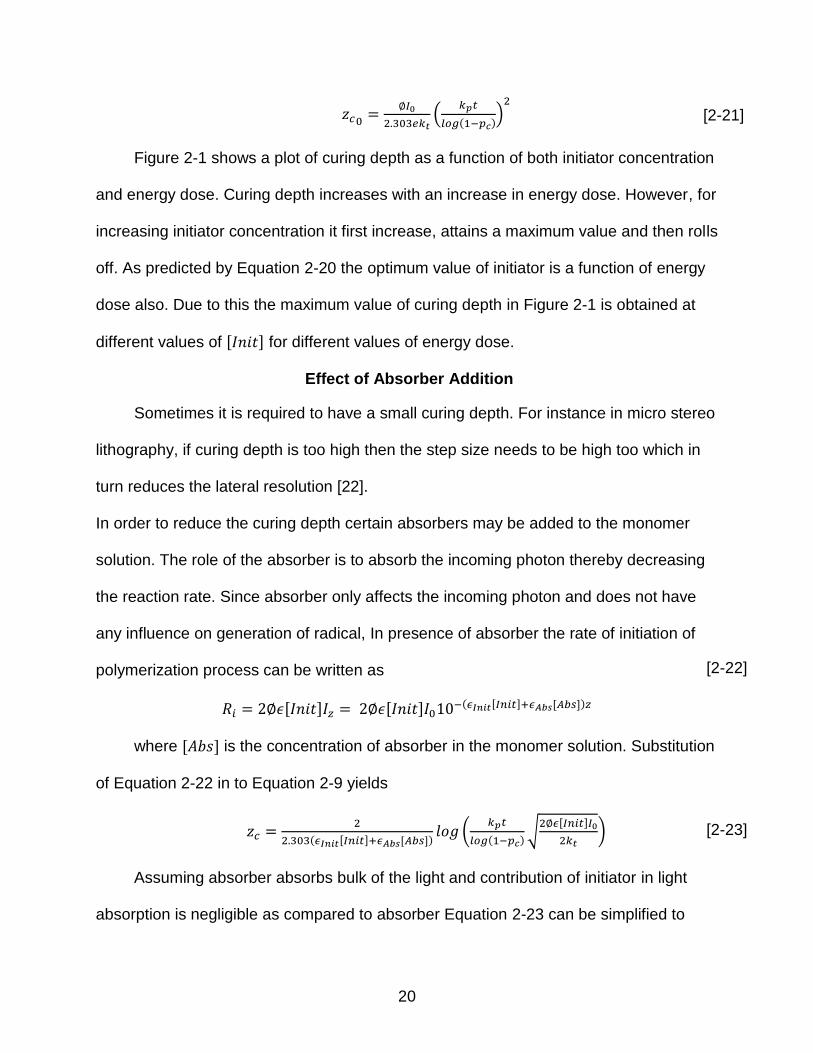
Figure 2-1 shows a plot of curing depth as a function of both initiator concentration

and energy dose. Curing depth increases with an increase in energy dose. However, for

increasing initiator concentration it first increase, attains a maximum value and then rolls

off. As predicted by Equation 2-20 the optimum value of initiator is a function of energy

dose also. Due to this the maximum value of curing depth in Figure 2-1 is obtained at

different values of [ ] for different values of energy dose.

Effect of Absorber Addition

Sometimes it is required to have a small curing depth. For instance in micro stereo

lithography, if curing depth is too high then the step size needs to be high too which in

turn reduces the lateral resolution [22].

In order to reduce the curing depth certain absorbers may be added to the monomer

solution. The role of the absorber is to absorb the incoming photon thereby decreasing

the reaction rate. Since absorber only affects the incoming photon and does not have

any influence on generation of radical, In presence of absorber the rate of initiation of

polymerization process can be written as

[ ] [ ] ( [ ] [ ])

where [ ] is the concentration of absorber in the monomer solution. Substitution

of Equation 2-22 in to Equation 2-9 yields

( [ ] [ ]) (

( )√

[ ]

)

Assuming absorber absorbs bulk of the light and contribution of initiator in light

absorption is negligible as compared to absorber Equation 2-23 can be simplified to

[2-21]

[2-22]

[2-23]

21

[ ] (

( )√

[ ]

)

Looking at Equation 2-24 it can be observed that curing depth is now a

monotonically increasing function of initiator concentration. Hence by using an absorber

curing depth can be controlled more accurately

Differentiating Equation 2-24 with respect to [ ] yields the maximum value of

[ ] up to which monotonicity is insured. The maximum value of [ ] is thus given by

[ ]

( ( )

)

(( [ ] [ ])

[ ])

[ ] ( [ ]

[ ])

Equation 2-25 predicts that by addition of absorber, the optimum value of [ ]

can be increased substantially and thus curing depth can be controlled more precisely

by changing the initiator concentration.

Effect of Temperature

Temperature plays a major role in the polymerization reaction rate. Reaction rate

can be increased exponentially by increasing the temperature. Since polymerization

reactions are usually exothermic, the temperature of monomer solution increases as

reaction proceeds further. This increased temperature can drastically change the curing

depth. Thus it is necessary to model the effect of temperature on curing depth model

derived in previous section. While deriving the curing depth equation, it was assumed

that except for [ ] every other parameter is temperature independent. However, this is

not quite the case. Both initiation rate and termination rate of radicals are altered by

changing the temperature of the monomer solution. The reaction rate constants of

radical initiation and termination are strong function of temperature. Their value

can be given by Arrhenius relationship

[2-24]

22

If the temperature of system changes with time, value of and also changes

with time. As the reaction proceeds, the temperature of the system increases due to

heat released by enthalpy of reaction. As the temperature increases, the reaction rate

increases and polymerization goes on deeper and deeper. By including the temperature

effect it is expected to have a larger value of curing depth as compared to the case

without temperature consideration.

The rate of increase of temperature can be computed by the total heat generated

by the polymerization reaction. If be the amount of heat generated per mole of the

polymer then

[ ]

( [ ]√

[ ] [ ]

)(

)

[ ]

[ ]√

[ ] [ ]

(

)

Inclusion of temperature dependence prohibits the derivation of a closed form

equation for curing depth. In order to compute curing depth as a function of time,

Equations 2-28 and 2-29 needs to be solved numerically. However, the curing depth

is not an independent variable, routine methods of solving ODE does not work here.

In order to obtain curing depth as function of time, curing depth is set to a

particular fixed value and then Equations 2-28 and 2-29 are iterated to obtain the time

required to reach the gel point. This method is then iterated for different values of curing

[2-26]

[2-27]

[2-29]

23

depth to plot curing depth as a function of time. The differential equations are solved in

MATLAB® using ode45 solver.

Figure 2-2 shows the curing depth as a function of time for different areas of

exposure. As the area of exposure is increased, curing depth increases drastically. As

the cuing depth is a strong function of temperature, if a smaller area is exposed the rise

in temperature is insignificant. For smaller area the curing depth is similar to as

predicted by Equation 2-8. For large area of exposure curing depth increases

significantly initially and then rolls off. The same behavior can be observed in

temperature profile also as shown in Figure 2-3.

Figure 2-3 shows the change in temperature as a function of time, it is interesting

to note that temperature starts to increase rapidly but then rolls off. The primary reason

behind such a behavior is the fact that as time passes by, more and more reaction goes

to completion and thus the heat generated rolls off as time passes by.

The strong temperature dependence can be observed by looking at T = 200 sec.

Even for a temperature difference of 150C the change in curing depth is more than 40%.

Also the % change in curing depth is at its maximum at start and then it keeps a

constant value. Both of these factors points to the fact that temperature plays a major

role in curing depth.

Experiment Setup

In order to verify the validity of curing depth model proposed, experimental study

of curing depth is performed. The monomer used for the curing depth study is HDDA

(Hexanediol Diacrylate). HDDA’s chemical structure is shown in Figure 2-4. The photo

initiator used is 2-hydroxy-2-methylpropiophenone and photo absorber used is 2-

hydroxy-4-(octyloxy)benzophenone. The chemical structure of photo initiator and

24

absorber is shown in Figure 2-4 A and 2-4 B. The concentration of photo initiator is

taken as 2% and 4% and concentration of absorber is taken as 1% and 3%. Mercury

lamp is used to produce illumination. The UV lamp produces monochromatic light of

wavelength 365nm with divergence less than 2.50.

The experimental setup for curing depth study is shown in Figure 2-5. A clear

glass plate is used as mask and is kept in contact with the monomer solution. The top

surface of the glass mask is covered with a UV blocking layer. A small square opening

of 1mm2 is cut at the center. The reason behind exposing a small area is to minimize

the temperature effects.

The UV light intensity is kept at its maximum value of 13.1mW/cm2. Exposure

dose is varied by opening the shutter for a variable time. Shutter is opened from 10s to

200s in the step of 10s. The resulting structure formed is then rinsed with methanol and

dried off by blowing nitrogen to remove any un-polymerized monomer. After rinsing the

thickness of polymer is measured using a screw gauge. The curing depth is then plotted

as a function of time and is shown in Figure 2-6 to Figure 2-9

Figure 2-6 and Figure 2-7 shows the curing depth as a function of time for different

initiator and absorber concentrations. It is readily visible that with an increase in initiator

concentration curing depth increases.

The dependence of initiator concentration on curing depth can be computed as

follows. Equation 2-6 can be simplified as follows.

[ ] (

( )√

[ ]

) ( )

[ ] (

( )

√

[ ] )

[2-30]

[2-31]

25

[ ]

[ ]

[ ]

[ ]

(√[ ]

[ ] )

For absorber = 1%, (B1/A1) – (B2/A2) yields 0.53 whereas log(√ ) has a value

equals 0.35.

For absorber = 3%, (B1/A1) – (B2/A2) yields 0.45 whereas log(√ ) has a value

equals 0.35. The slight discrepancy is due to the fact that curing depth is computed

using steady state assumption which gives rise to square root dependence. When

steady state is not obtained initiator will have dependence which is greater than square

root as rate of initiation is higher than rate of termination.

Figure 2-9 shows the curing depth as a function of time for different absorber

concentration. It is readily visible that with an increase in absorber concentration curing

depth decreases.

In order to understand the significance of curing depth, another experiment for

constant curing depth is performed. If two different solutions have same curing depth

then the resulting polymerized structure would be the same. The overall process does

not depend on the individual absorber and initiator concentration but depends upon the

curing depth. In order to validate this hypothesis Two monomer solutions, one having

1% initiator and 2% initiator and other having 3% absorber and 2% initiator are taken.

Their curing depth curve is shown in Figure 2-10

These two solutions are irradiated to the UV light of intensity 13.1mW/cm2 with an

area of exposure of 1mm2. The mask contains two types of pattern which results in

holes of 82µm and 164µm diameter with 100µm and 200µm of pitch and posts of the

same dimensions as holes.

[2-32]

26

The two monomer solution were irradiated for same amount of time = 100s.

Solution of low absorber has a very high curing depth and thus results in loss of

features. The results are shown in Figure 2-11. Also the loss of feature is more

pronounced in the structure with lower feature size.

Solution having 3% absorber and 4% initiator is abbreviated as Solution 1 and

Solution having 1% absorber and 2% initiator is abbreviated as Solution 2.

The case for constant curing depth is shown in Figure 2-12. The solution with

lower absorber concentration is irradiated for a smaller period of time. Looking at the

Fig2-9 for a constant curing depth of 100µm, Solution 1 is exposed for 20sec and

solution 2 is exposed for 100 sec. The resulting structure is shown in Figure 2-12

By observing Figure 2-12 it can be said that both the solutions resulted in similar

looking structures. However, the exposure time is greatly reduced for solution with low

absorber concentration. It is evident from Figure 2-11 and Figure 2-12 that curing depth

is among the most important parameter for polymerization process. If two monomer

solutions have same curing depth then they will result in similar looking structures

despite having entirely different absorber and Initiator concentrations.

Curing depth can be tuned by varying initiator and absorber concentrations,

however, addition of absorber makes the tuning easy. An increase in absorber

concentration will decrease the curing depth and increase in initiator concentration will

increase the curing depth. Their dependence is derived analytically in Equation 2-24.

Another important parameter is the temperature of monomer solution. It has

exponential dependence on rate of reaction and thus it can change the curing depth

substantially. The situation is exacerbated by the fact that temperature provides a

27

positive feedback and thus a large increase in curing depth is observed at the start of

the reaction. This behavior result in print through error if a large area is exposed and

temperature consideration is not taken into account.

28

Figure 2-1. Curing Depth as a function of both initiator and energy dose. The parameters used to generate this image are taken from. [12]

0

0.001

0.002

0.003

0.004

0.005

1,0

00

6,0

00

11

,00

0

16

,00

0

21

,00

0

26

,00

0

31

,00

0

36

,00

0

41

,00

0

46

,00

0

Initiator Conc. in mol/L Energy in J/m2

10-1

10-2

10-3

10-4

29

Figure 2-2. Curing Depth as a function of time and area of exposure. The red curve shows the curing depth for an exposed area of 1mm2, the blue curve shows the curing depth for an exposed area of 10mm2 and the green line shows the curing depth for an exposed area of 1cm2.

0

20

40

60

80

100

120

140

160

180

200

0 200 400 600 800 1000

Cu

rin

g D

ep

th in

µm

Time in Sec

30

Figure 2-3. Temperature as a function of time and area of exposure. The red curve shows the curing depth for an exposed area of 1mm2, the blue curve shows the curing depth for an exposed area of 10mm2 and the green line shows the curing depth for an exposed area of 1cm2.

295

300

305

310

315

320

325

330

335

0 200 400 600 800 1000

Te

mp

era

ture

in

K

Time in Sec

31

Figure 2-4. Chemical structure of A) cis-7,cis-11-Hexadecadienyl acetate B) 2-hydroxy-2-methylpropiophenone and C) 2-hydroxy-4-(octyloxy) benzophenone [23].

Figure 2-5. Experimental setup used for curing depth study.

A

B

C

32

Figure 2-6. Curing depth as a function of time for constant intensity exposure and absorber concentration of 1%. The black line shows the logarithmic fit and its Equation is shown next to the curve.

y = 77.047ln(x) - 139.08

y = 85.712ln(x) - 109.57

0

50

100

150

200

250

300

350

400

0 50 100 150 200

Cu

rin

g D

ep

th in

µm

Time in Sec

A = 1%, I = 2%

A = 1%, I = 4%

33

Figure 2-7. Curing depth as a function of time for constant intensity exposure and absorber concentration of 3%. The black line shows the logarithmic fit and its Equation is shown next to the curve.

y = 32.779ln(x) - 71.037

y = 34.896ln(x) - 59.415

0

20

40

60

80

100

120

140

0 50 100 150 200 250 300

Cu

rin

g D

ep

th in

µm

Time in Sec

A = 3%, I = 2%

A = 3%, I = 4%

34

Figure 2-8. Curing depth as a function of time for constant intensity exposure and initiator concentration of 2%. The black line shows the logarithmic fit and its Equation is shown next to the curve.

y = 77.047ln(x) - 139.08

y = 32.779ln(x) - 71.037

0

50

100

150

200

250

300

0 50 100 150 200 250 300

Cu

rin

g D

ep

th in

µm

Time in Sec

A = 1%, I = 2%

A = 3%, I = 2%

35

Figure 2-9. Curing depth as a function of time for constant intensity exposure and initiator concentration of 4%. The black line shows the logarithmic fit and its Equation is shown next to the curve.

y = 85.712ln(x) - 109.57

y = 34.896ln(x) - 59.415

0

50

100

150

200

250

300

350

400

0 50 100 150 200

Cu

rin

g D

ep

th in

µm

Time in Sec

A = 1%, I = 4%

A = 3%, I = 4%

36

Figure 2-10. Curing depth as a function of time for constant intensity exposure. The two solutions have both different initiator and absorber concentration.

y = 77.047ln(x) - 139.08

y = 34.896ln(x) - 59.415

0

50

100

150

200

250

300

0 50 100 150 200

Cu

rin

g D

ep

th in

µm

Time in Sec

A = 1%, I = 2%

A = 3%, I = 4%

37

Figure 2-11. Result for constant exposure time of 100 sec. A1: Posts of 164µm diameter at 20X mag. for Solution 1. A2: Posts of 164µm diameter at 20X mag. for Solution 2. B1: Holes of 82µm diameter at 20X mag. for Solution 1. B2: Holes of 82µm diameter at 20X mag. for Solution 2. C1: Posts of 82µm diameter at 20X mag. for Solution 1. C2: Posts of 82µm diameter at 20X mag. for Solution 2. D1: Holes of 164µm diameter at 20X mag. for Solution 1. D2: Holes of 164µm diameter at 20X mag. for Solution 2.

Figure 2-12. Result for constant curing depth of 100 µm. A1: Posts of 164µm diameter at 20X mag. for Solution 1. A2: Posts of 164µm diameter at 20X mag. for Solution 2. B1: Holes of 82µm diameter at 20X mag. for Solution 1. B2: Holes of 82µm diameter at 20X mag. for Solution 2. C1: Posts of 82µm diameter at 20X mag. for Solution 1. C2: Posts of 82µm diameter at 20X mag. for Solution 2. D1: Holes of 164µm diameter at 20X mag. for Solution 1. D2: Holes of 164µm diameter at 20X mag. for Solution 2.

A1 A2 B1 B2

C1 C2 D1 D2

A1 B1

C1 D1 D2 C2

B2 A2

38

CHAPTER 3 DIVERGENCE STUDY

In proximity micro stereo lithography it is required to maintain the monomer top

layer and mask in close proximity (~50-100 µm) to overcome the divergence of

collimated light source. However, maintaining such a small gap during a polymerization

run is troublesome. A number of factors can disturb the top layer of monomer and cause

the monomer and mask surface to be in contact. Some of the factors are vibration due

to stepper motor and curling due to stress in the polymer structure. These factors further

reduce the gap as the polymerization reaction proceeds making it more susceptible to

unwanted contact.

The value of divergence angle of light source sets up a maximum value of the

separation between mask and monomer layer. If monomer is beyond that limit, spatial

resolution of resulting structure will be distorted or in a worst scenario everything will be

exposed uniformly. To understand it more clearly consider the case shown in Figure 3-

2. The mask consists of UV blocking holes as shown in Figure 3-1. The UV light is

convergent with an angle of . The diameter of resulting holes is shown as a function of

depth. It is interesting to note that diameter of holes first increases and then starts

decreasing. Also when it obtains its maximum value the light can also start making

diffraction patterns which will result in distorted shape.

Experimental Setup

In order to quantify the result, a divergence study is performed. Si wafers are

coated with SU-8 photoresist. It is a negative photoresist, used to make high aspect

ratio structures. SU-8 has a maximum absorption at 365 nm which coincides with the

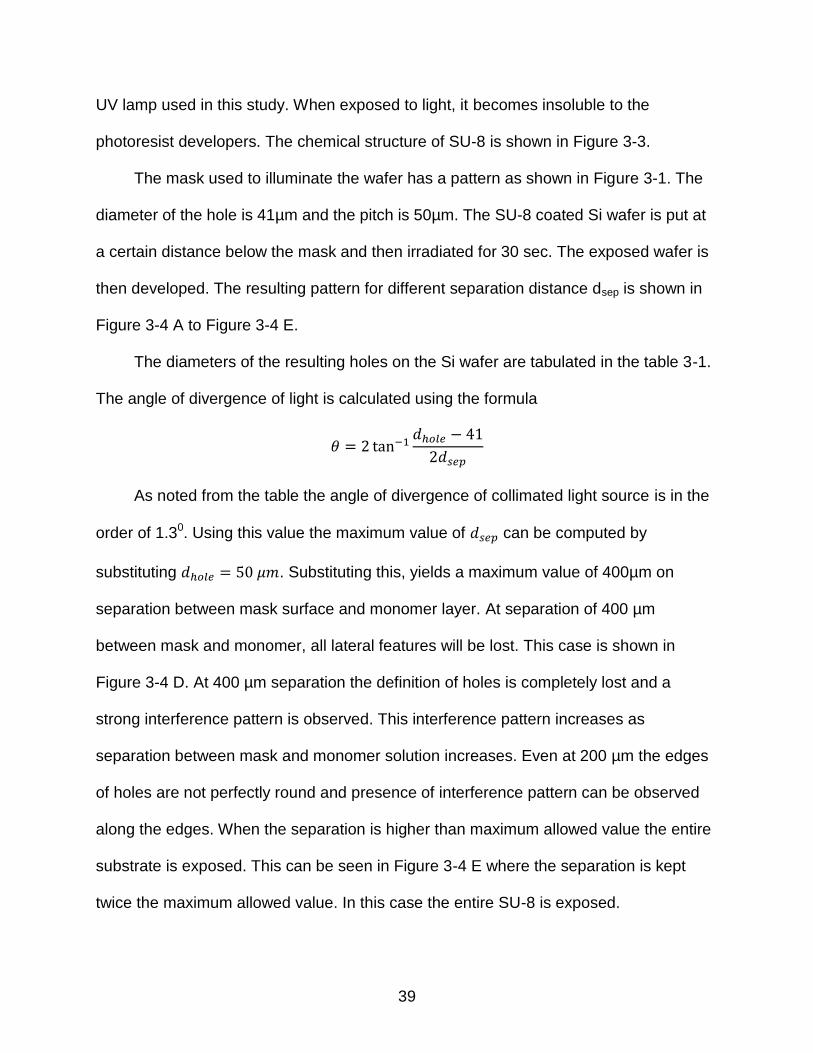
39

UV lamp used in this study. When exposed to light, it becomes insoluble to the

photoresist developers. The chemical structure of SU-8 is shown in Figure 3-3.

The mask used to illuminate the wafer has a pattern as shown in Figure 3-1. The

diameter of the hole is 41µm and the pitch is 50µm. The SU-8 coated Si wafer is put at

a certain distance below the mask and then irradiated for 30 sec. The exposed wafer is

then developed. The resulting pattern for different separation distance dsep is shown in

Figure 3-4 A to Figure 3-4 E.

The diameters of the resulting holes on the Si wafer are tabulated in the table 3-1.

The angle of divergence of light is calculated using the formula

As noted from the table the angle of divergence of collimated light source is in the

order of 1.30. Using this value the maximum value of can be computed by

substituting . Substituting this, yields a maximum value of 400µm on

separation between mask surface and monomer layer. At separation of 400 µm

between mask and monomer, all lateral features will be lost. This case is shown in

Figure 3-4 D. At 400 µm separation the definition of holes is completely lost and a

strong interference pattern is observed. This interference pattern increases as

separation between mask and monomer solution increases. Even at 200 µm the edges

of holes are not perfectly round and presence of interference pattern can be observed

along the edges. When the separation is higher than maximum allowed value the entire

substrate is exposed. This can be seen in Figure 3-4 E where the separation is kept

twice the maximum allowed value. In this case the entire SU-8 is exposed.

40

Divergence study becomes extremely useful to set the gap between mask and

monomer layer. Since this gap is constrained by divergence of light source and also

since the effect of interference increases with an increase in separation, a smaller value

of gap is preferred. For typical cases the gap desired is usually tens to hundreds of

micron. However, maintaining such a small gap during the polymerization process is a

big challenge. Numerous factors can change the gap between mask and monomer and

may result in unintentional contact between the two. The surface roughness of substrate

itself is usually few tens of microns. It results in a big challenge to obtain a gap which is

of the same order. Meniscus effect on edges also poses a challenge to obtain such a

small gap. Apart from these factors the gap between mask and monomer layer changes

during the polymerization process also. A very small vibration can cause a contact

between mask and monomer layer. Also as polymerization process happens a new

monomer layer comes on top of polymerized structure which further reduces the gap.

Also if during the polymerization process if polymerized part is not fully cured and is

under stress, it may bend and cause the monomer solution to contact the mask surface.

Taking these factors into consideration, the gap between monomer and mask can

not be fixed to an arbitrary small value. As seen from the results, the lateral feature size

does not degrade if the gap is kept less than half the maximum allowed gap. The

divergence study not only provides an upper bound on the gap between mask and

monomer but also provides the range on which the lateral resolution is preserved.

41

Table 3-1. Experimentally computed angle of convergence at different depth

Separation in um Diameter of hole in um Angle of Divergence in 0

50 42 1.160

100 43.2 1.260

200 45.4 1.260

Figure 3-1. Profile of mask having walls between holes as opaque to UV.

Figure 3-2. Diameter of Hole as a function of Depth.

Figure 3-3. Chemical Structure of SU-8 Photoresist [24].

42

Figure 3-4. Structure developed on SU-8 coated wafer as a function of distance. A: dsep = 50µm, B: dsep = 100µm, C: dsep = 200µm, D: dsep = 400µm, E: dsep = 800µm,

B

A

A

D C

E

43

CHAPTER 4 CONCLUSION

Among the various parameters to characterize and control a polymerization

process, curing depth is one of the most important parameter. It is directly responsible

for the minimum lateral feature size. Hence to obtain a particular cross section, curing

depth needs to be controlled very precisely. Also to avoid excess polymerization via

punch through error, per step displacement and exposure dose is determined by curing

depth and thus it has to be controlled accurately. An extensive mathematical model of

curing depth is presented in this work. The effect of initiator and energy dose is derived

and optimal curing depth is computed. As initiator has a complex dependence on curing

depth, controlling the curing depth by just varying initiator is difficult. The optimal curing

depth is not only a function of initiator but also of energy dose. In order to tune the

curing depth more accurately, absorber is added so that effect of initiator is simplified.

With the addition of absorber curing depth can be increased or decreased more

accurately by increasing or decreasing the concentration of initiator or absorber. The

mathematical model incorporating all of these factors is derived and verified using

experimental results. The strong dependence of curing depth on lateral resolution also

suggests that two solutions with similar curing depths will produce similar structure. This

property of curing depth is verified using experimental results. These results suggest

that monomer solution behaves according to curing depth which is a combination of

both initiator and absorber concentration rather than their individual concentrations.

Another important parameter in characterizing micro stereo lithography is the

divergence of collimated light source. This divergence sets the maximum allowable limit

on the mask – monomer separation without loss of lateral feature size. The effect of

44

increasing separation on lateral feature size is demonstrated. This study not only

provides an upper limit on allowable gap but also the safe region of operation to ensure

lateral resolution is not distorted.

These two parameters are two of the most parameters in a micro stereo

lithohgraphy process. These parameters can be used to obtain the value of different

variables such as initiator and absorber concentration, exposure dose, step size and

gap between mask and monomer. These are the main parameters in a lithography

process. By performing a curing depth and divergence study, these parameters can be

set accurately which will result in more accurate polymerization process.

45

LIST OF REFERENCES

[1] S.M. Sze, Semiconductor Sensors, Wiley, New York, 1994.

[2] E.W. Becker, W. Ehrfeld, P. Hagmann, A. Maner, D. Munchmeyer, Fabrication of microstructures with high aspect ratios and great structural heights by synchrotron radiation lithography, galvanoforming, and plastic moulding (LIGA process), Microelectronic Engineering, Volume 4, Issue 1, May 1986, Pages 35-56

[3] K. Williams, J. Maxwell, K. Larsson, M. Boman, Freeform fabrication of functional microsolenoids, electromagnets and helical springs using high-pressure laser chemical vapor deposition , Micro Electro Mechanical Systems, 1999. MEMS '99.Twelfth IEEE International Conference on , vol., no., pp.232-237, 17-21 Jan 1999

[4] A. Cohen, G. Zhang, F.-G Tseng, U. Frodis, F. Mansfeld, P. Will, EFAB: rapid, low-cost desktop micromachining of high aspect ratio true 3-D MEMS, Micro Electro Mechanical Systems, 1999. MEMS '99. Twelfth IEEE International Conference on , vol., no., pp.244-251, 17-21 Jan 1999

[5] Hull, C. (1986), Apparatus for Production of Three-Dimensional Objects by Stereolithography, U.S. Pat. No. 4575330

[6] S. Maruo, K. Ikuta, Movable microstructures made by two-photon three-dimensional microfabrication, Micromechatronics and Human Science, 1999. MHS '99. Proceedings of 1999 International Symposium on , vol., no., pp.173-178, 1999

[7] X. Zhang, X. N. Jiang, C. Sun, Micro-stereolithography of polymeric and ceramic microstructures, Sensors and Actuators A: Physical, Volume 77, Issue 2, 12 October 1999, Pages 149-156

[8] A. Bertsch, S. Jiguet, P. Bernhard, P. Renaud, Microstereolithography: a Review, Materials Research Society Symposium Proceedings, Volume 758, 2002

[9] A. Bertsch, S. Zissi, J. Y. Jézéquel, S. Corbel, and J. C. André. Microstereophotolithography using a liquid crystal display as dynamic mask-generator. Microsystem Technologies 3, no. 2 (February 25, 1997): 42-47.

[10] Beluze, Laurence, Arnaud Bertsch, and Philippe Renaud. Microstereolithography: a new process to build complex 3D objects. In Design, Test, and Microfabrication of MEMS and MOEMS, edited by Bernard Courtois, Selden B. Crary, Wolfgang Ehrfeld, Hiroyuki Fujita, Jean Michel Karam, and Karen W. Markus, 3680:808-817. Paris, France: SPIE, 1999.

[11] M. Alonso, Optimization of a light emitting diode based projection stereolithography system and its applications, Micro, 2010.

46

[12] J.H. Lee, R.K. Prud'homme and I.A. Aksay, Cure depth in photopolymerization: experiments and theory, J Mater Res 16 (2001), pp. 3536–3544

[13] X. Zhang, X. N. Jiang, C. Sun, Micro-stereolithography of polymeric and ceramic microstructures, Sensors and Actuators A: Physical, Volume 77, Issue 2, 12 October 1999, Pages 149-156

[14] S. Maruo, K. Ikuta, Movable microstructures made by two-photon three-dimensional microfabrication, Micromechatronics and Human Science, 1999. MHS '99. Proceedings of 1999 International Symposium on , vol., no., pp.173-178, 1999

[15] J.P. Fouassier, Photoinitiation, Photopolymerization, and Photocuring (Hanser, Cincinnati, OH, 1995).

[16] J.P. Fouassier and J.F. Rabek, Radiation Curing in Polymer Science and Technology (Elsevier, New York, 1993).

[17] G.G. Odian, Principles of Polymerization, 3rd ed. (Wiley, New York, 1991).

[18] J.H. Lambert, Photometrie (Augsburg, Germany, 1760).

[19] A. Beer, Ann. Physik Chem. 2, 78 (1852).

[20] S.P. Obukhov, M. Rubinstein and R.H. Colby, Network Modulus and Superelasticity, Macromolecules, Volume 27, Issue 12, Pages 3191-3198, 1994

[21] Hale, Arturo, Macosko, Christopher W. and Bair, Harvey E, Glass transition temperature as a function of conversion in thermosetting polymers, Macromolecules, Volume 24, Issue 9, Pages 2610-2621, 1991

[22] C. Sun, N. Fang, D.M. Wu, X. Zhang, Projection micro-stereolithography using digital micro-mirror dynamic mask, Sensors and Actuators A: Physical, Volume 121, Issue 1, 31 May 2005, Pages 113-120

[23] http://www.sigmaaldrich.com

[24] http://www.microchem.com/products/su_eight.htm

47

BIOGRAPHICAL SKETCH

Abhinav Pandey is a graduate student at University of Florida in Electrical and

Computer Engineering. He received his Master of Science degree from University of

Florida in spring 2011. He received his Bachelor of Technology degree from Indian

Institute of Technology, Kanpur in Electrical Engineering in 2009.