Business object data services ds 42_tutorial_en
142
PUBLIC SAP Data Services Document Version: 4.2 Support Package 5 (14.2.5.0) – 2015-05-05 Tutorial
-
Upload
duskydope-rao -
Category
Technology
-
view
12 -
download
1
Transcript of Business object data services ds 42_tutorial_en

PUBLIC
SAP Data ServicesDocument Version: 4.2 Support Package 5 (14.2.5.0) – 2015-05-05
Tutorial

Content
1 Introduction. . . . . . . . . . . . . . . . . . . . . . . . . . . . . . . . . . . . . . . . . . . . . . . . . . . . . . . . . . . . . . . . . . 71.1 Audience and assumptions. . . . . . . . . . . . . . . . . . . . . . . . . . . . . . . . . . . . . . . . . . . . . . . . . . . . . . . . .71.2 SAP information resources. . . . . . . . . . . . . . . . . . . . . . . . . . . . . . . . . . . . . . . . . . . . . . . . . . . . . . . . .71.3 Tutorial objectives. . . . . . . . . . . . . . . . . . . . . . . . . . . . . . . . . . . . . . . . . . . . . . . . . . . . . . . . . . . . . . . 81.4 Tutorial prerequisites. . . . . . . . . . . . . . . . . . . . . . . . . . . . . . . . . . . . . . . . . . . . . . . . . . . . . . . . . . . . 9
Preparation for this tutorial. . . . . . . . . . . . . . . . . . . . . . . . . . . . . . . . . . . . . . . . . . . . . . . . . . . . . . 9Environment required. . . . . . . . . . . . . . . . . . . . . . . . . . . . . . . . . . . . . . . . . . . . . . . . . . . . . . . . . . 9Tutorial setup. . . . . . . . . . . . . . . . . . . . . . . . . . . . . . . . . . . . . . . . . . . . . . . . . . . . . . . . . . . . . . . 9
1.5 Tutorial structure. . . . . . . . . . . . . . . . . . . . . . . . . . . . . . . . . . . . . . . . . . . . . . . . . . . . . . . . . . . . . . .161.6 Exiting the tutorial. . . . . . . . . . . . . . . . . . . . . . . . . . . . . . . . . . . . . . . . . . . . . . . . . . . . . . . . . . . . . . 17
Resuming the tutorial. . . . . . . . . . . . . . . . . . . . . . . . . . . . . . . . . . . . . . . . . . . . . . . . . . . . . . . . . 18
2 Product Overview . . . . . . . . . . . . . . . . . . . . . . . . . . . . . . . . . . . . . . . . . . . . . . . . . . . . . . . . . . . . . 192.1 Product features. . . . . . . . . . . . . . . . . . . . . . . . . . . . . . . . . . . . . . . . . . . . . . . . . . . . . . . . . . . . . . . 192.2 Product components. . . . . . . . . . . . . . . . . . . . . . . . . . . . . . . . . . . . . . . . . . . . . . . . . . . . . . . . . . . . 202.3 Using the product. . . . . . . . . . . . . . . . . . . . . . . . . . . . . . . . . . . . . . . . . . . . . . . . . . . . . . . . . . . . . . 212.4 System configurations. . . . . . . . . . . . . . . . . . . . . . . . . . . . . . . . . . . . . . . . . . . . . . . . . . . . . . . . . . . 22
Windows implementation. . . . . . . . . . . . . . . . . . . . . . . . . . . . . . . . . . . . . . . . . . . . . . . . . . . . . . 23UNIX implementation. . . . . . . . . . . . . . . . . . . . . . . . . . . . . . . . . . . . . . . . . . . . . . . . . . . . . . . . . 23
2.5 The Designer window. . . . . . . . . . . . . . . . . . . . . . . . . . . . . . . . . . . . . . . . . . . . . . . . . . . . . . . . . . . . 232.6 Objects. . . . . . . . . . . . . . . . . . . . . . . . . . . . . . . . . . . . . . . . . . . . . . . . . . . . . . . . . . . . . . . . . . . . . .24
Object hierarchy. . . . . . . . . . . . . . . . . . . . . . . . . . . . . . . . . . . . . . . . . . . . . . . . . . . . . . . . . . . . . 25Object-naming conventions. . . . . . . . . . . . . . . . . . . . . . . . . . . . . . . . . . . . . . . . . . . . . . . . . . . . .28
2.7 New terms. . . . . . . . . . . . . . . . . . . . . . . . . . . . . . . . . . . . . . . . . . . . . . . . . . . . . . . . . . . . . . . . . . . 282.8 Section summary and what to do next. . . . . . . . . . . . . . . . . . . . . . . . . . . . . . . . . . . . . . . . . . . . . . . . 29
3 Defining Source and Target Metadata . . . . . . . . . . . . . . . . . . . . . . . . . . . . . . . . . . . . . . . . . . . . . 303.1 Logging in to the Designer. . . . . . . . . . . . . . . . . . . . . . . . . . . . . . . . . . . . . . . . . . . . . . . . . . . . . . . . 303.2 Defining a datastore. . . . . . . . . . . . . . . . . . . . . . . . . . . . . . . . . . . . . . . . . . . . . . . . . . . . . . . . . . . . 30
Defining a datastore for the source (ODS) database. . . . . . . . . . . . . . . . . . . . . . . . . . . . . . . . . . . . 31Defining a datastore for the target database. . . . . . . . . . . . . . . . . . . . . . . . . . . . . . . . . . . . . . . . . 33
3.3 Importing metadata. . . . . . . . . . . . . . . . . . . . . . . . . . . . . . . . . . . . . . . . . . . . . . . . . . . . . . . . . . . . .33Importing metadata for ODS source tables . . . . . . . . . . . . . . . . . . . . . . . . . . . . . . . . . . . . . . . . . .33Importing metadata for target tables. . . . . . . . . . . . . . . . . . . . . . . . . . . . . . . . . . . . . . . . . . . . . . 34
3.4 Defining a file format. . . . . . . . . . . . . . . . . . . . . . . . . . . . . . . . . . . . . . . . . . . . . . . . . . . . . . . . . . . . 343.5 New terms. . . . . . . . . . . . . . . . . . . . . . . . . . . . . . . . . . . . . . . . . . . . . . . . . . . . . . . . . . . . . . . . . . . 363.6 Summary and what to do next. . . . . . . . . . . . . . . . . . . . . . . . . . . . . . . . . . . . . . . . . . . . . . . . . . . . . 37
2P U B L I C© 2015 SAP SE or an SAP affiliate company. All rights reserved.
TutorialContent

4 Populating the SalesOrg Dimension from a Flat File. . . . . . . . . . . . . . . . . . . . . . . . . . . . . . . . . . . 384.1 Objects and their hierarchical relationships. . . . . . . . . . . . . . . . . . . . . . . . . . . . . . . . . . . . . . . . . . . . 384.2 Adding a new project. . . . . . . . . . . . . . . . . . . . . . . . . . . . . . . . . . . . . . . . . . . . . . . . . . . . . . . . . . . . 394.3 Adding a job. . . . . . . . . . . . . . . . . . . . . . . . . . . . . . . . . . . . . . . . . . . . . . . . . . . . . . . . . . . . . . . . . . 394.4 About work flows. . . . . . . . . . . . . . . . . . . . . . . . . . . . . . . . . . . . . . . . . . . . . . . . . . . . . . . . . . . . . . .39
Adding a work flow. . . . . . . . . . . . . . . . . . . . . . . . . . . . . . . . . . . . . . . . . . . . . . . . . . . . . . . . . . . 404.5 About data flows. . . . . . . . . . . . . . . . . . . . . . . . . . . . . . . . . . . . . . . . . . . . . . . . . . . . . . . . . . . . . . . 41
Adding a data flow. . . . . . . . . . . . . . . . . . . . . . . . . . . . . . . . . . . . . . . . . . . . . . . . . . . . . . . . . . . .41Defining the data flow. . . . . . . . . . . . . . . . . . . . . . . . . . . . . . . . . . . . . . . . . . . . . . . . . . . . . . . . . 43Validating the data flow. . . . . . . . . . . . . . . . . . . . . . . . . . . . . . . . . . . . . . . . . . . . . . . . . . . . . . . . 45Addressing errors. . . . . . . . . . . . . . . . . . . . . . . . . . . . . . . . . . . . . . . . . . . . . . . . . . . . . . . . . . . .46
4.6 Saving the project. . . . . . . . . . . . . . . . . . . . . . . . . . . . . . . . . . . . . . . . . . . . . . . . . . . . . . . . . . . . . . 464.7 Executing the job. . . . . . . . . . . . . . . . . . . . . . . . . . . . . . . . . . . . . . . . . . . . . . . . . . . . . . . . . . . . . . .464.8 About deleting objects. . . . . . . . . . . . . . . . . . . . . . . . . . . . . . . . . . . . . . . . . . . . . . . . . . . . . . . . . . . 494.9 New terms. . . . . . . . . . . . . . . . . . . . . . . . . . . . . . . . . . . . . . . . . . . . . . . . . . . . . . . . . . . . . . . . . . . 494.10 Summary and what to do next. . . . . . . . . . . . . . . . . . . . . . . . . . . . . . . . . . . . . . . . . . . . . . . . . . . . . 49
5 Populating the Time Dimension Using a Transform. . . . . . . . . . . . . . . . . . . . . . . . . . . . . . . . . . . .505.1 Retrieving the project. . . . . . . . . . . . . . . . . . . . . . . . . . . . . . . . . . . . . . . . . . . . . . . . . . . . . . . . . . . 50
Opening the Class_Exercises project. . . . . . . . . . . . . . . . . . . . . . . . . . . . . . . . . . . . . . . . . . . . . . .515.2 Adding the job and data flow. . . . . . . . . . . . . . . . . . . . . . . . . . . . . . . . . . . . . . . . . . . . . . . . . . . . . . . 515.3 Defining the time dimension data flow. . . . . . . . . . . . . . . . . . . . . . . . . . . . . . . . . . . . . . . . . . . . . . . . 51
Specifying the components of the time data flow. . . . . . . . . . . . . . . . . . . . . . . . . . . . . . . . . . . . . . 51Defining the flow of data. . . . . . . . . . . . . . . . . . . . . . . . . . . . . . . . . . . . . . . . . . . . . . . . . . . . . . . 52Defining the output of the Date_Generation transform. . . . . . . . . . . . . . . . . . . . . . . . . . . . . . . . . . 52Defining the output of the query. . . . . . . . . . . . . . . . . . . . . . . . . . . . . . . . . . . . . . . . . . . . . . . . . .53
5.4 Saving and executing the job. . . . . . . . . . . . . . . . . . . . . . . . . . . . . . . . . . . . . . . . . . . . . . . . . . . . . . 535.5 Summary and what to do next. . . . . . . . . . . . . . . . . . . . . . . . . . . . . . . . . . . . . . . . . . . . . . . . . . . . . 54
6 Populating the Customer Dimension from a Relational Table. . . . . . . . . . . . . . . . . . . . . . . . . . . . 556.1 Adding the CustDim job and work flow. . . . . . . . . . . . . . . . . . . . . . . . . . . . . . . . . . . . . . . . . . . . . . . .556.2 Adding the CustDim data flow. . . . . . . . . . . . . . . . . . . . . . . . . . . . . . . . . . . . . . . . . . . . . . . . . . . . . .566.3 Defining the CustDim data flow. . . . . . . . . . . . . . . . . . . . . . . . . . . . . . . . . . . . . . . . . . . . . . . . . . . . . 56
Bringing the objects into the data flow. . . . . . . . . . . . . . . . . . . . . . . . . . . . . . . . . . . . . . . . . . . . . 56Defining the query. . . . . . . . . . . . . . . . . . . . . . . . . . . . . . . . . . . . . . . . . . . . . . . . . . . . . . . . . . . 57
6.4 Validating the CustDim data flow. . . . . . . . . . . . . . . . . . . . . . . . . . . . . . . . . . . . . . . . . . . . . . . . . . . .576.5 Executing the CustDim job. . . . . . . . . . . . . . . . . . . . . . . . . . . . . . . . . . . . . . . . . . . . . . . . . . . . . . . . 576.6 Using the interactive debugger. . . . . . . . . . . . . . . . . . . . . . . . . . . . . . . . . . . . . . . . . . . . . . . . . . . . . 58
Setting a breakpoint in a data flow. . . . . . . . . . . . . . . . . . . . . . . . . . . . . . . . . . . . . . . . . . . . . . . . 58Using the interactive debugger. . . . . . . . . . . . . . . . . . . . . . . . . . . . . . . . . . . . . . . . . . . . . . . . . . 59Setting a breakpoint condition. . . . . . . . . . . . . . . . . . . . . . . . . . . . . . . . . . . . . . . . . . . . . . . . . . . 60
6.7 Summary and what to do next. . . . . . . . . . . . . . . . . . . . . . . . . . . . . . . . . . . . . . . . . . . . . . . . . . . . . .61
TutorialContent
P U B L I C© 2015 SAP SE or an SAP affiliate company. All rights reserved. 3

7 Populating the Material Dimension from an XML File. . . . . . . . . . . . . . . . . . . . . . . . . . . . . . . . . . 627.1 Adding MtrlDim job, work and data flows. . . . . . . . . . . . . . . . . . . . . . . . . . . . . . . . . . . . . . . . . . . . . . 627.2 Importing a document type definition. . . . . . . . . . . . . . . . . . . . . . . . . . . . . . . . . . . . . . . . . . . . . . . . 637.3 Defining the MtrlDim data flow. . . . . . . . . . . . . . . . . . . . . . . . . . . . . . . . . . . . . . . . . . . . . . . . . . . . . 63
Adding the objects to the data flow. . . . . . . . . . . . . . . . . . . . . . . . . . . . . . . . . . . . . . . . . . . . . . . .63Defining the details of qryunnest. . . . . . . . . . . . . . . . . . . . . . . . . . . . . . . . . . . . . . . . . . . . . . . . . 64
7.4 Validating that the MtrlDim data flow has been constructed properly. . . . . . . . . . . . . . . . . . . . . . . . . . 657.5 Executing the MtrlDim job. . . . . . . . . . . . . . . . . . . . . . . . . . . . . . . . . . . . . . . . . . . . . . . . . . . . . . . . 667.6 Leveraging the XML_Pipeline . . . . . . . . . . . . . . . . . . . . . . . . . . . . . . . . . . . . . . . . . . . . . . . . . . . . . . 66
Setting up a job and data flow that uses the XML_Pipeline transform. . . . . . . . . . . . . . . . . . . . . . . .66Defining the details of XML_Pipeline and Query_Pipeline. . . . . . . . . . . . . . . . . . . . . . . . . . . . . . . . 67
7.7 Summary and what to do next. . . . . . . . . . . . . . . . . . . . . . . . . . . . . . . . . . . . . . . . . . . . . . . . . . . . . 68
8 Populating the Sales Fact Table from Multiple Relational Tables. . . . . . . . . . . . . . . . . . . . . . . . . 708.1 Exercise overview. . . . . . . . . . . . . . . . . . . . . . . . . . . . . . . . . . . . . . . . . . . . . . . . . . . . . . . . . . . . . . 708.2 Adding the SalesFact job, work flow, and data flow. . . . . . . . . . . . . . . . . . . . . . . . . . . . . . . . . . . . . . . 718.3 Defining the SalesFact data flow. . . . . . . . . . . . . . . . . . . . . . . . . . . . . . . . . . . . . . . . . . . . . . . . . . . . 718.4 Defining the details of the Query transform. . . . . . . . . . . . . . . . . . . . . . . . . . . . . . . . . . . . . . . . . . . . 728.5 Defining the details of the lookup_ext function. . . . . . . . . . . . . . . . . . . . . . . . . . . . . . . . . . . . . . . . . . 73
Using a lookup_ext function for order status. . . . . . . . . . . . . . . . . . . . . . . . . . . . . . . . . . . . . . . . . 738.6 Validating the SalesFact data flow. . . . . . . . . . . . . . . . . . . . . . . . . . . . . . . . . . . . . . . . . . . . . . . . . . . 758.7 Executing the SalesFact job. . . . . . . . . . . . . . . . . . . . . . . . . . . . . . . . . . . . . . . . . . . . . . . . . . . . . . . 758.8 Viewing Impact and Lineage Analysis for the SALES_FACT target table. . . . . . . . . . . . . . . . . . . . . . . . 758.9 Summary and what to do next. . . . . . . . . . . . . . . . . . . . . . . . . . . . . . . . . . . . . . . . . . . . . . . . . . . . . .77
9 Changed-Data Capture. . . . . . . . . . . . . . . . . . . . . . . . . . . . . . . . . . . . . . . . . . . . . . . . . . . . . . . . . 789.1 Exercise overview. . . . . . . . . . . . . . . . . . . . . . . . . . . . . . . . . . . . . . . . . . . . . . . . . . . . . . . . . . . . . . 789.2 Adding and defining the initial-load job. . . . . . . . . . . . . . . . . . . . . . . . . . . . . . . . . . . . . . . . . . . . . . . .78
Adding the job and defining global variables. . . . . . . . . . . . . . . . . . . . . . . . . . . . . . . . . . . . . . . . . 79Adding and defining the work flow. . . . . . . . . . . . . . . . . . . . . . . . . . . . . . . . . . . . . . . . . . . . . . . . 79
9.3 Adding and defining the delta-load job. . . . . . . . . . . . . . . . . . . . . . . . . . . . . . . . . . . . . . . . . . . . . . . . 81Adding the delta-load data flow. . . . . . . . . . . . . . . . . . . . . . . . . . . . . . . . . . . . . . . . . . . . . . . . . . 82Adding the job and defining the global variables. . . . . . . . . . . . . . . . . . . . . . . . . . . . . . . . . . . . . . .82Adding and defining the work flow. . . . . . . . . . . . . . . . . . . . . . . . . . . . . . . . . . . . . . . . . . . . . . . . 82Defining the scripts. . . . . . . . . . . . . . . . . . . . . . . . . . . . . . . . . . . . . . . . . . . . . . . . . . . . . . . . . . .83
9.4 Executing the jobs. . . . . . . . . . . . . . . . . . . . . . . . . . . . . . . . . . . . . . . . . . . . . . . . . . . . . . . . . . . . . . 83Executing the initial-load job. . . . . . . . . . . . . . . . . . . . . . . . . . . . . . . . . . . . . . . . . . . . . . . . . . . . 83Changing the source data. . . . . . . . . . . . . . . . . . . . . . . . . . . . . . . . . . . . . . . . . . . . . . . . . . . . . . 84Executing the delta-load job. . . . . . . . . . . . . . . . . . . . . . . . . . . . . . . . . . . . . . . . . . . . . . . . . . . . 84
9.5 Summary and what to do next. . . . . . . . . . . . . . . . . . . . . . . . . . . . . . . . . . . . . . . . . . . . . . . . . . . . . 84
10 Data Assessment. . . . . . . . . . . . . . . . . . . . . . . . . . . . . . . . . . . . . . . . . . . . . . . . . . . . . . . . . . . . . 86
4P U B L I C© 2015 SAP SE or an SAP affiliate company. All rights reserved.
TutorialContent
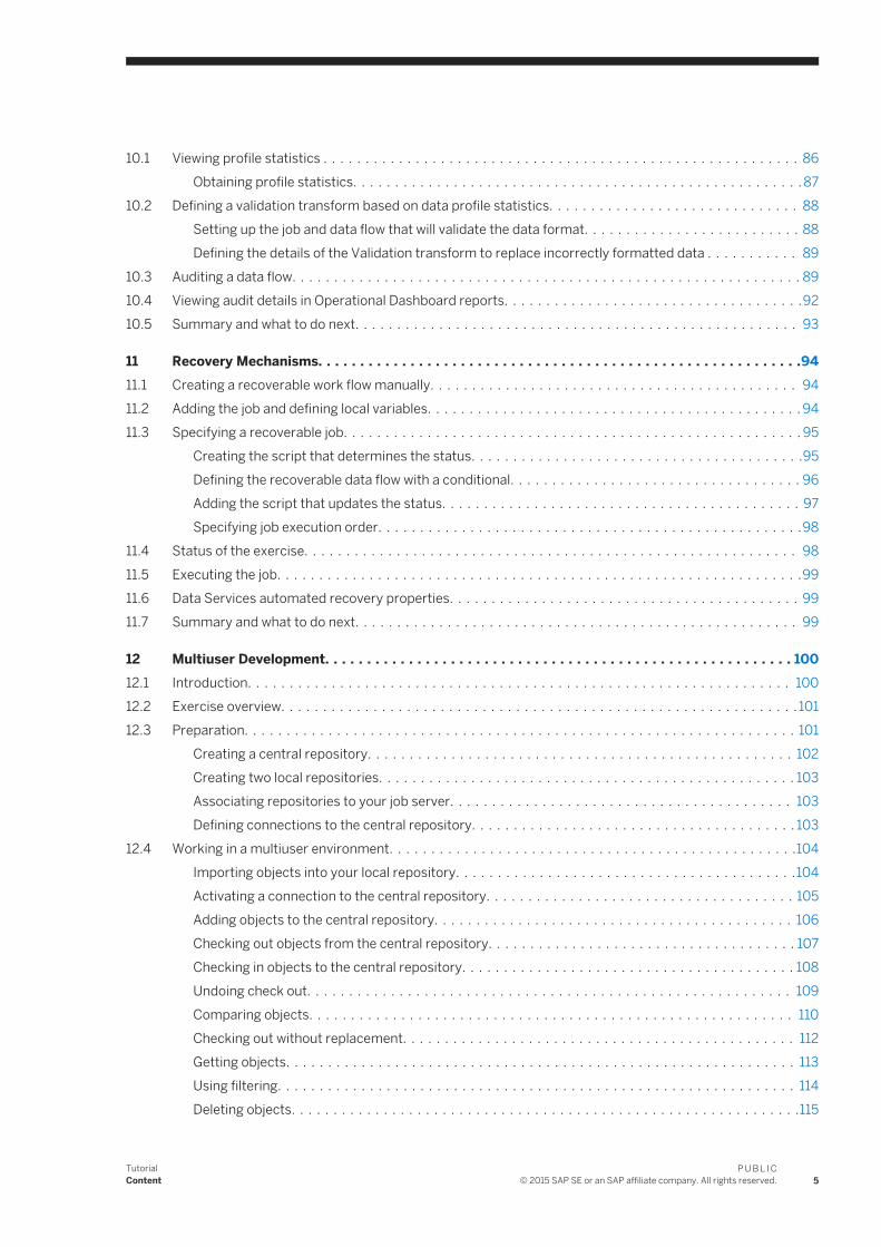
10.1 Viewing profile statistics . . . . . . . . . . . . . . . . . . . . . . . . . . . . . . . . . . . . . . . . . . . . . . . . . . . . . . . . . 86Obtaining profile statistics. . . . . . . . . . . . . . . . . . . . . . . . . . . . . . . . . . . . . . . . . . . . . . . . . . . . . . 87
10.2 Defining a validation transform based on data profile statistics. . . . . . . . . . . . . . . . . . . . . . . . . . . . . . 88Setting up the job and data flow that will validate the data format. . . . . . . . . . . . . . . . . . . . . . . . . . 88Defining the details of the Validation transform to replace incorrectly formatted data . . . . . . . . . . . 89
10.3 Auditing a data flow. . . . . . . . . . . . . . . . . . . . . . . . . . . . . . . . . . . . . . . . . . . . . . . . . . . . . . . . . . . . . 8910.4 Viewing audit details in Operational Dashboard reports. . . . . . . . . . . . . . . . . . . . . . . . . . . . . . . . . . . .9210.5 Summary and what to do next. . . . . . . . . . . . . . . . . . . . . . . . . . . . . . . . . . . . . . . . . . . . . . . . . . . . . 93
11 Recovery Mechanisms. . . . . . . . . . . . . . . . . . . . . . . . . . . . . . . . . . . . . . . . . . . . . . . . . . . . . . . . . .9411.1 Creating a recoverable work flow manually. . . . . . . . . . . . . . . . . . . . . . . . . . . . . . . . . . . . . . . . . . . . 9411.2 Adding the job and defining local variables. . . . . . . . . . . . . . . . . . . . . . . . . . . . . . . . . . . . . . . . . . . . . 9411.3 Specifying a recoverable job. . . . . . . . . . . . . . . . . . . . . . . . . . . . . . . . . . . . . . . . . . . . . . . . . . . . . . . 95
Creating the script that determines the status. . . . . . . . . . . . . . . . . . . . . . . . . . . . . . . . . . . . . . . .95Defining the recoverable data flow with a conditional. . . . . . . . . . . . . . . . . . . . . . . . . . . . . . . . . . . 96Adding the script that updates the status. . . . . . . . . . . . . . . . . . . . . . . . . . . . . . . . . . . . . . . . . . . 97Specifying job execution order. . . . . . . . . . . . . . . . . . . . . . . . . . . . . . . . . . . . . . . . . . . . . . . . . . .98
11.4 Status of the exercise. . . . . . . . . . . . . . . . . . . . . . . . . . . . . . . . . . . . . . . . . . . . . . . . . . . . . . . . . . . 9811.5 Executing the job. . . . . . . . . . . . . . . . . . . . . . . . . . . . . . . . . . . . . . . . . . . . . . . . . . . . . . . . . . . . . . .9911.6 Data Services automated recovery properties. . . . . . . . . . . . . . . . . . . . . . . . . . . . . . . . . . . . . . . . . . 9911.7 Summary and what to do next. . . . . . . . . . . . . . . . . . . . . . . . . . . . . . . . . . . . . . . . . . . . . . . . . . . . . 99
12 Multiuser Development. . . . . . . . . . . . . . . . . . . . . . . . . . . . . . . . . . . . . . . . . . . . . . . . . . . . . . . . 10012.1 Introduction. . . . . . . . . . . . . . . . . . . . . . . . . . . . . . . . . . . . . . . . . . . . . . . . . . . . . . . . . . . . . . . . . 10012.2 Exercise overview. . . . . . . . . . . . . . . . . . . . . . . . . . . . . . . . . . . . . . . . . . . . . . . . . . . . . . . . . . . . . . 10112.3 Preparation. . . . . . . . . . . . . . . . . . . . . . . . . . . . . . . . . . . . . . . . . . . . . . . . . . . . . . . . . . . . . . . . . . 101
Creating a central repository. . . . . . . . . . . . . . . . . . . . . . . . . . . . . . . . . . . . . . . . . . . . . . . . . . . 102Creating two local repositories. . . . . . . . . . . . . . . . . . . . . . . . . . . . . . . . . . . . . . . . . . . . . . . . . . 103Associating repositories to your job server. . . . . . . . . . . . . . . . . . . . . . . . . . . . . . . . . . . . . . . . . 103Defining connections to the central repository. . . . . . . . . . . . . . . . . . . . . . . . . . . . . . . . . . . . . . . 103
12.4 Working in a multiuser environment. . . . . . . . . . . . . . . . . . . . . . . . . . . . . . . . . . . . . . . . . . . . . . . . .104Importing objects into your local repository. . . . . . . . . . . . . . . . . . . . . . . . . . . . . . . . . . . . . . . . .104Activating a connection to the central repository. . . . . . . . . . . . . . . . . . . . . . . . . . . . . . . . . . . . . 105Adding objects to the central repository. . . . . . . . . . . . . . . . . . . . . . . . . . . . . . . . . . . . . . . . . . . 106Checking out objects from the central repository. . . . . . . . . . . . . . . . . . . . . . . . . . . . . . . . . . . . . 107Checking in objects to the central repository. . . . . . . . . . . . . . . . . . . . . . . . . . . . . . . . . . . . . . . . 108Undoing check out. . . . . . . . . . . . . . . . . . . . . . . . . . . . . . . . . . . . . . . . . . . . . . . . . . . . . . . . . . 109Comparing objects. . . . . . . . . . . . . . . . . . . . . . . . . . . . . . . . . . . . . . . . . . . . . . . . . . . . . . . . . . 110Checking out without replacement. . . . . . . . . . . . . . . . . . . . . . . . . . . . . . . . . . . . . . . . . . . . . . . 112Getting objects. . . . . . . . . . . . . . . . . . . . . . . . . . . . . . . . . . . . . . . . . . . . . . . . . . . . . . . . . . . . . 113Using filtering. . . . . . . . . . . . . . . . . . . . . . . . . . . . . . . . . . . . . . . . . . . . . . . . . . . . . . . . . . . . . . 114Deleting objects. . . . . . . . . . . . . . . . . . . . . . . . . . . . . . . . . . . . . . . . . . . . . . . . . . . . . . . . . . . . .115
TutorialContent
P U B L I C© 2015 SAP SE or an SAP affiliate company. All rights reserved. 5

12.5 Summary and what to do next. . . . . . . . . . . . . . . . . . . . . . . . . . . . . . . . . . . . . . . . . . . . . . . . . . . . . 116
13 Extracting SAP Application Data. . . . . . . . . . . . . . . . . . . . . . . . . . . . . . . . . . . . . . . . . . . . . . . . . 11713.1 Defining an SAP Applications datastore. . . . . . . . . . . . . . . . . . . . . . . . . . . . . . . . . . . . . . . . . . . . . . 11713.2 Importing metadata for individual SAP application source tables. . . . . . . . . . . . . . . . . . . . . . . . . . . . 11813.3 Repopulating the customer dimension table. . . . . . . . . . . . . . . . . . . . . . . . . . . . . . . . . . . . . . . . . . . 119
Adding the SAP_CustDim job, work flow, and data flow. . . . . . . . . . . . . . . . . . . . . . . . . . . . . . . . . 119Defining the SAP_CustDim data flow. . . . . . . . . . . . . . . . . . . . . . . . . . . . . . . . . . . . . . . . . . . . . . 119Defining the ABAP data flow. . . . . . . . . . . . . . . . . . . . . . . . . . . . . . . . . . . . . . . . . . . . . . . . . . . . 121Validating the SAP_CustDim data flow. . . . . . . . . . . . . . . . . . . . . . . . . . . . . . . . . . . . . . . . . . . . 124Executing the SAP_CustDim job. . . . . . . . . . . . . . . . . . . . . . . . . . . . . . . . . . . . . . . . . . . . . . . . . 124About ABAP job execution errors. . . . . . . . . . . . . . . . . . . . . . . . . . . . . . . . . . . . . . . . . . . . . . . . 124
13.4 Repopulating the material dimension table. . . . . . . . . . . . . . . . . . . . . . . . . . . . . . . . . . . . . . . . . . . . 125Adding the SAP_MtrlDim job, work flow, and data flow. . . . . . . . . . . . . . . . . . . . . . . . . . . . . . . . . 125Defining the DF_SAP_MtrlDim data flow. . . . . . . . . . . . . . . . . . . . . . . . . . . . . . . . . . . . . . . . . . . 126Defining the data flow. . . . . . . . . . . . . . . . . . . . . . . . . . . . . . . . . . . . . . . . . . . . . . . . . . . . . . . . 126Executing the SAP_MtrlDim job. . . . . . . . . . . . . . . . . . . . . . . . . . . . . . . . . . . . . . . . . . . . . . . . . 129
13.5 Repopulating the SalesFact table. . . . . . . . . . . . . . . . . . . . . . . . . . . . . . . . . . . . . . . . . . . . . . . . . . .129Adding the SAP_SalesFact job, work flow, and data flow. . . . . . . . . . . . . . . . . . . . . . . . . . . . . . . . 129Defining the DF_SAP_SalesFact data flow. . . . . . . . . . . . . . . . . . . . . . . . . . . . . . . . . . . . . . . . . . 130Defining the ABAP data flow. . . . . . . . . . . . . . . . . . . . . . . . . . . . . . . . . . . . . . . . . . . . . . . . . . . .130Validating the SAP_SalesFact data flow and executing the job. . . . . . . . . . . . . . . . . . . . . . . . . . . . 135
13.6 New Terms. . . . . . . . . . . . . . . . . . . . . . . . . . . . . . . . . . . . . . . . . . . . . . . . . . . . . . . . . . . . . . . . . . 13513.7 Summary. . . . . . . . . . . . . . . . . . . . . . . . . . . . . . . . . . . . . . . . . . . . . . . . . . . . . . . . . . . . . . . . . . . 136
14 Running a Real-time Job in Test Mode. . . . . . . . . . . . . . . . . . . . . . . . . . . . . . . . . . . . . . . . . . . . . 13714.1 Exercise. . . . . . . . . . . . . . . . . . . . . . . . . . . . . . . . . . . . . . . . . . . . . . . . . . . . . . . . . . . . . . . . . . . . 137
6P U B L I C© 2015 SAP SE or an SAP affiliate company. All rights reserved.
TutorialContent
1 Introduction
Welcome to the Tutorial. This tutorial introduces core features of SAP Data Services. The software is a component of the SAP Information Management solutions and allows you to extract and integrate data for analytical reporting and e-business.
Exercises in this tutorial introduce concepts and techniques to extract, transform, and load batch data from flat-file and relational database sources for use in a data warehouse. Additionally, you can use the software for real-time data extraction and integration. Use this tutorial to gain practical experience using software components including the Designer, repositories, and Job Servers.
SAP Information Management solutions also provide a number of Rapid Marts packages, which are predefined data models with built-in jobs for use with business intelligence (BI) and online analytical processing (OLAP) tools. Contact your sales representative for more information about Rapid Marts.
1.1 Audience and assumptions
This tutorial assumes that:
● You are an application developer or database administrator working on data extraction, data warehousing, data integration, or data quality.
● You understand your source data systems, DBMS, business intelligence, and e-business messaging concepts.● You understand your organization's data needs.● You are familiar with SQL (Structured Query Language).● You are familiar with Microsoft Windows.
1.2 SAP information resources
A list of information resource links.
A global network of SAP technology experts provides customer support, education, and consulting to ensure maximum information management benefit to your business.
Useful addresses at a glance:
Table 1:
Address Content
Customer Support, Consulting, and Education services
http://service.sap.com/
Information about SAP Business User Support programs, as well as links to technical articles, downloads, and online discussions.
TutorialIntroduction
P U B L I C© 2015 SAP SE or an SAP affiliate company. All rights reserved. 7
Address Content
Product documentation
http://help.sap.com/bods/
SAP product documentation.
SAP Data Services tutorial
http://help.sap.com/businessobject/product_guides/sbods42/en/ds_42_tutorial_en.pdf
Introduces core features, concepts and techniques to extract, transform, and load batch data from flat-file and relational database sources for use in a data warehouse.
SAP Data Services Community Network
http://scn.sap.com/community/data-services
Get online and timely information about SAP Data Services, including forums, tips and tricks, additional downloads, samples, and much more. All content is to and from the community, so feel free to join in and contact us if you have a submission.
EIM Wiki page on SCN
http://wiki.sdn.sap.com/wiki/display/EIM/EIM+Home
The means with which to contribute content, post comments, and organize information in a hierarchical manner to so that information is easy to find.
Supported Platforms (Product Availability Matrix)
https://service.sap.com/PAM
Information about supported platforms for SAP Data Services with a search function to quickly find information related to your platform.
Blueprints
http://scn.sap.com/docs/DOC-8820
Blueprints for you to download and modify to fit your needs. Each blueprint contains the necessary SAP Data Services project, jobs, data flows, file formats, sample data, template tables, and custom functions to run the data flows in your environment with only a few modifications.
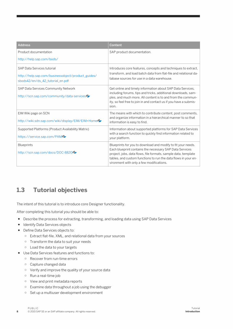
1.3 Tutorial objectives
The intent of this tutorial is to introduce core Designer functionality.
After completing this tutorial you should be able to:
● Describe the process for extracting, transforming, and loading data using SAP Data Services● Identify Data Services objects● Define Data Services objects to:
○ Extract flat-file, XML, and relational data from your sources○ Transform the data to suit your needs○ Load the data to your targets
● Use Data Services features and functions to:○ Recover from run-time errors○ Capture changed data○ Verify and improve the quality of your source data○ Run a real-time job○ View and print metadata reports○ Examine data throughout a job using the debugger○ Set up a multiuser development environment
8P U B L I C© 2015 SAP SE or an SAP affiliate company. All rights reserved.
TutorialIntroduction
1.4 Tutorial prerequisites
This section provides a high-level description of the steps you need to complete before you begin the tutorial exercises.
1.4.1 Preparation for this tutorial
Read the sections on logging in to the Designer and the Designer user interface in the SAP Data Services Designer Guide to get an overview of the Designer user interface including terms and concepts relevant to this tutorial.
This tutorial also provides a high-level summary in the next section, Product Overview.
1.4.2 Environment required
To use this tutorial, you must have Data Services running on a supported version of Windows and a supported RDBMS (such as Oracle, IBM DB2, Microsoft SQL Server, or SAP Sybase SQL Anywhere).
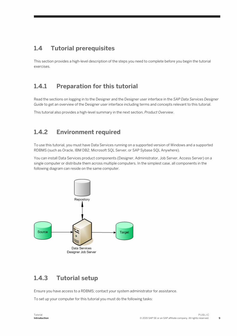
You can install Data Services product components (Designer, Administrator, Job Server, Access Server) on a single computer or distribute them across multiple computers. In the simplest case, all components in the following diagram can reside on the same computer.
1.4.3 Tutorial setup
Ensure you have access to a RDBMS; contact your system administrator for assistance.
To set up your computer for this tutorial you must do the following tasks:
TutorialIntroduction
P U B L I C© 2015 SAP SE or an SAP affiliate company. All rights reserved. 9
● Creating repository, source, and target databases on an existing RDBMS [page 10]● Installing SAP Data Services [page 11]● Running the provided SQL scripts to create sample source and target tables [page 15]
1.4.3.1 Creating repository, source, and target databases on an existing RDBMS
1. Log in to your RDBMS.2. (Oracle only). Optionally create a service name alias.
Set the protocol to TCP/IP and enter a service name; for example, training.sap. This can act as your connection name.
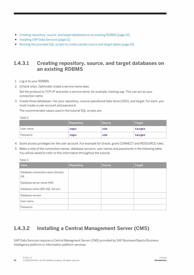
3. Create three databases—for your repository, source operational data store (ODS), and target. For each, you must create a user account and password.The recommended values used in the tutorial SQL scripts are:
Table 2:
Repository Source Target
User name repo ods target
Password repo ods target
4. Grant access privileges for the user account. For example for Oracle, grant CONNECT and RESOURCE roles.5. Make a note of the connection names, database versions, user names and passwords in the following table.
You will be asked to refer to this information throughout the tutorial.
Table 3:
Value Repository Source Target
Database connection name (Oracle) OR
Database server name AND
Database name (MS-SQL Server)
Database version
User name
Password
1.4.3.2 Installing a Central Management Server (CMS)
SAP Data Services requires a Central Managment Server (CMS) provided by SAP BusinessObjects Business Intelligence platform or Information platform services.
10P U B L I C© 2015 SAP SE or an SAP affiliate company. All rights reserved.
TutorialIntroduction

For detailed information about system requirements, configuration, and installation for Information platform services, see the “Installing Information platform services” section of the Installation Guide for Windows.
For detailed information about system requirements, configuration, and installation for SAP BusinessObjects Business Intelligence platform , see the SAP BusinessObjects Business Intelligence platform Installation Guide.
NoteDuring installation, make a note of the administrator user name and password for the SAP BusinessObjects Business Intelligence platform or Information platform services system. You will be asked to enter it to complete the setup of the tutorial.
1.4.3.2.1 Logging in to the Central Management Console
To configure user accounts and define Data Services repositories, log in to the Central Management Console (CMC).
1. Navigate to http://<hostname>:8080/BOE/CMC/, where <hostname> is the name of the machine where you installed SAP BusinessObjects Business Intelligence platform or Information platform services.
2. Enter the username, password, and authentication type for your CMS user.3. Click Log On.
The Central Management Console main screen is displayed.
1.4.3.3 Installing SAP Data Services
For detailed information about system requirements, configuration, and installing on Windows or UNIX, See the Installation Guide for Windows or Installation Guide for UNIX.
Be prepared to enter the following information when installing the software:
● Your Windows domain and user name● Your Windows password● Your Windows computer name and host ID● Product keycode● Connection information for the local repository and Job Server
When you install the software, it configures a Windows service for the Job Server. To verify that the service is enabled, open the Services Control Panel and ensure that all Data Services services are configured for a Status of Started and Startup Type Automatic.
The default installation creates the following entries in the Start Programs SAP Data Services 4.2 menu:
Table 4:
Command Function
Data Services Designer Opens the Designer.
TutorialIntroduction
P U B L I C© 2015 SAP SE or an SAP affiliate company. All rights reserved. 11

Command Function
Data Services Locale Selector Allows you to specify the language, territory, and code page to use for the repository connection for Designer and to process job data
Data Services Management Console
Opens a launch page for the Data Services web applications including the Administrator and metadata and data quality reporting tools.
Data Services Repository Manager
Opens a dialog box that you can use to update repository connection information.
Data Services Server Manager Opens a dialog box that you can use to configure Job Servers and Access Servers.
License Manager Displays license information.
1.4.3.3.1 Creating a local repository
1. Open the Repository Manager.2. Choose Local as the repository type.3. Enter the connection information for the local repository database that you created.4. Type repo for both User and Password.
5. Click Create.
After creating the repository, you need to define a Job Server and associate the repository with it. You can also optionally create an Access Server if you want to use web-based batch job administration.
1.4.3.3.2 Defining a job server and associating your repository
1. Open the Server Manager.2. In the Job Server tab of the Server Manager window, click Configuration Editor.3. In the Job Server Configuration Editor window, click Add to add a Job Server.4. In the Job Server Properties window:
a. Enter a unique name in Job Server name.b. For Job Server port, enter a port number that is not used by another process on the computer. If you are
unsure of which port number to use, increment the default port number.c. You do not need to complete the other job server properties to run the exercises in this Tutorial.
5. Under Associated Repositories, enter the local repository to associate with this Job Server. Every Job Server must be associated with at least one local repository.a. Click Add to associate a new local or profiler repository with this Job Server.b. Under Repository information enter the connection information for the local repository database that you
created.c. Type repo for both Username and Password.d. Select the Default repository check box if this is the default repository for this Job Server. You cannot
specify more than one default repository.
12P U B L I C© 2015 SAP SE or an SAP affiliate company. All rights reserved.
TutorialIntroduction

e. Click Apply to save your entries. You should see <database_server>_repo_repo in the list of Associated Repositories.
6. Click OK to close the Job Server Properties window.7. Click OK to close the Job Server Configuration Editor window.8. Click Close and Restart in the Server Manager.9. Click OK to confirm that you want to restart the Data Services Service.
1.4.3.3.3 Creating a new Data Services user account
Before you can log in to the Designer, you need to create a user account on the Central Management Server (CMS).
1. Log in to the Central Management Console (CMC) using the Administrator account you created during installation.
2. Click Users and Groups.The user management screen is displayed.
3. Click Manage New New User .The New User screen is displayed.
4. Enter user details for the new user account:
Table 5:
Field Value
Authentication Type Enterprise
Account Name tutorial_user
Full Name Tutorial User
Description User created for the Data Services tutorial.
Password tutorial_pass
Password never expires Checked
User must change password at next logon Unchecked
5. Click Create & Close.The user account is created and the New User screen is closed.
6. Add your user to the necessary Data Services user groups:a. Click User List.b. Select tutorial_user in the list of users.
c. Choose Actions Join Group .The Join Group screen is displayed.
d. Select all the Data Services groups and click >.
TutorialIntroduction
P U B L I C© 2015 SAP SE or an SAP affiliate company. All rights reserved. 13

CautionThis simplifies the process for the purposes of the tutorial. In a production environment, you should plan user access more carefully. For more information about user security, see the Administrator Guide.
The Data Services groups are moved to the Destination Groups area.e. Click OK.
The Join Group screen is closed.7. Click Log Off to exit the Central Management Console.
Related Information
Logging in to the Central Management Console [page 11]
1.4.3.3.4 Configuring the local repository in the CMC
Before you can grant repository access to your user, you need to configure the repository in the Central Management Console (CMC).
1. Log in to the Central Management Console using the tutorial user you created.2. Click Data Services.
The Data Services management screen is displayed.
3. Click Manage Configure Repository .The Add Data Services Repository screen is displayed.
4. Enter a name for the repository.For example, Tutorial Repository.
5. Enter the connection information for the database you created for the local repository.6. Click Test Connection.
A dialog appears indicating whether or not the connection to the repository database was successful. Click OK. If the connection failed, verify your database connection information and re-test the connection.
7. Click Save.The Add Data Services Repository screen closes.
8. Click the Repositories folder.The list of configured repositories is displayed. Verify that the new repository is shown.
9. Click Log Off to exit the Central Management Console.
Related Information
Logging in to the Central Management Console [page 11]
14P U B L I C© 2015 SAP SE or an SAP affiliate company. All rights reserved.
TutorialIntroduction
1.4.3.4 Running the provided SQL scripts to create sample source and target tables
Data Services installation includes a batch file (CreateTables_<databasetype>.bat) for each supported RDBMS. The batch files run SQL scripts that create and populate tables on your source database and create the target schema on the target database.
1. Using Windows Explorer, locate the CreateTables batch file for your RDBMS in your Data Services installation directory in <LINK_DIR>\Tutorial Files\Scripts.
2. Open the appropriate script file and edit the pertinent connection information (and user names and passwords if you are not using ods/ods and target/target).
The Oracle batch file contains commands of the form:
sqlplus <username/password@connection @scriptfile>.sql > <outputfile>.out
The Microsoft SQL Server batch file contains commands of the form:
isql /e /n /U <username> /S <servername> /d <databasename> /P <password> /i <scriptfile>.sql /o <outputfile>.out
NoteFor Microsoft SQL Server 2008, use CreateTables_MSSQL2005.bat.
The output files provide logs that you can examine for success or error messages.3. Double-click on the batch file to run the SQL scripts.4. Use an RDBMS query tool to check your source ODS database.
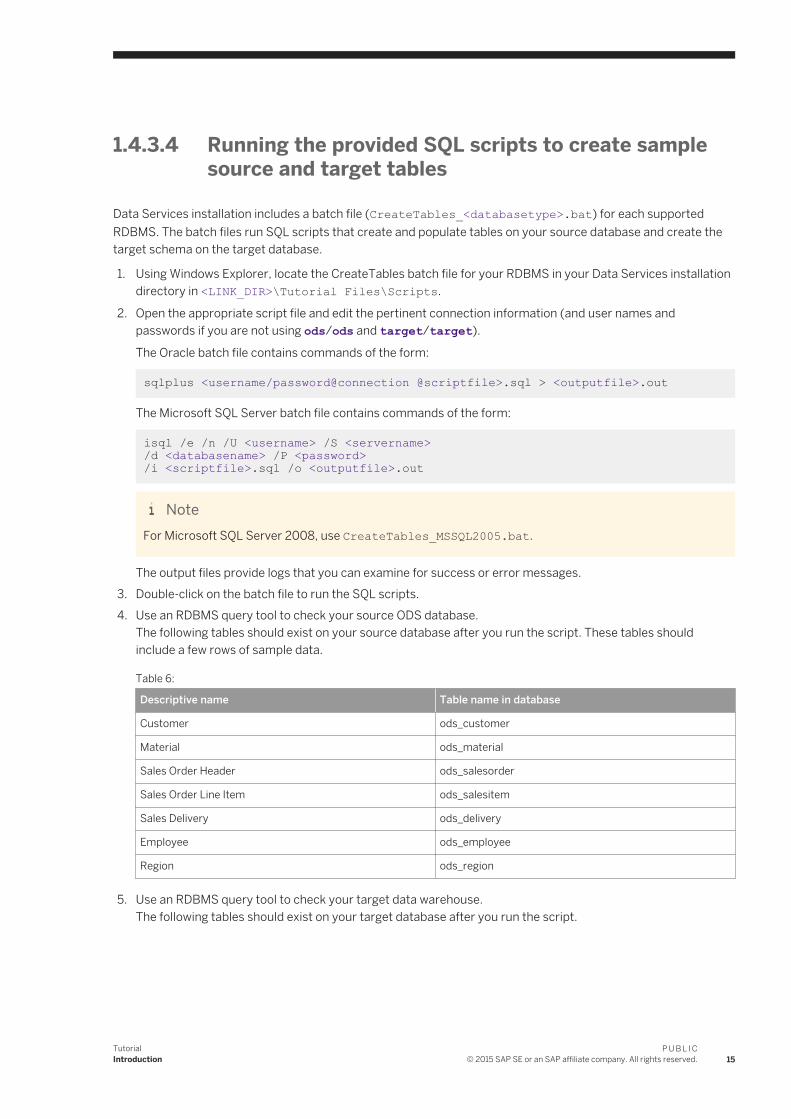
The following tables should exist on your source database after you run the script. These tables should include a few rows of sample data.
Table 6:
Descriptive name Table name in database
Customer ods_customer
Material ods_material
Sales Order Header ods_salesorder
Sales Order Line Item ods_salesitem
Sales Delivery ods_delivery
Employee ods_employee
Region ods_region
5. Use an RDBMS query tool to check your target data warehouse.The following tables should exist on your target database after you run the script.
TutorialIntroduction
P U B L I C© 2015 SAP SE or an SAP affiliate company. All rights reserved. 15

Table 7:
Descriptive name Table name in database
Sales Org Dimension salesorg_dim
Customer Dimension cust_dim
Material Dimension mtrl_dim
Time Dimension time_dim
Employee Dimension employee_dim
Sales Fact sales_fact
Recovery Status status_table
CDC Status CDC_time
1.5 Tutorial structure
The goal of the tutorial exercises is to demonstrate SAP Data Services features using a simplified data model. The model is a sales data warehouse with a star schema that contains one fact table and some dimension tables.
Sections build on jobs you create and skills learned in previous sections. You must complete each exercise to begin the next.
NoteThe screens in this guide are for illustrative purposes. On some screens, the available options depend on the database type and version in the environment.
This tutorial is organized as follows.
Product Overview introduces the basic architecture and the user interface for Data Services.
16P U B L I C© 2015 SAP SE or an SAP affiliate company. All rights reserved.
TutorialIntroduction

Defining Source and Target Metadata introduces working with the Designer. Use the Designer to define a datastore and a file format, then import metadata to the object library. After completing this section, you will have completed the preliminary work required to define data movement specifications for flat-file data.
Populating the SalesOrg Dimension from a Flat File introduces basic data flows, query transforms, and source and target tables. The exercise populates the sales organization dimension table from flat-file data.
Populating the Time Dimension Using a Transform introduces Data Services functions. This exercise creates a data flow for populating the time dimension table.
Populating the Customer Dimension from a Relational Table introduces data extraction from relational tables. This exercise defines a job that populates the customer dimension table.
Populating the Material Dimension from an XML File introduces data extraction from nested sources. This exercise defines a job that populates the material dimension table.
Populating the Sales Fact Table from Multiple Relational Tables continues data extraction from relational tables and introduces joins and the lookup function. The exercise populates the sales fact table.
Changed-Data Capture introduces a basic approach to changed-data capture. The exercise uses variables, parameters, functions, and scripts.
Data Assessment introduces features to ensure and improve the validity of your source data. The exercise uses profile statistics, the validation transform, and the audit data flow feature.
Recovery Mechanisms presents techniques for recovering from incomplete data loads.
Multiuser Development presents the use of a central repository for setting up a multiuser development environment.
Extracting SAP Application Data provides optional exercises on extracting data from SAP application sources.
Running a Real-time Job in Test Mode provides optional exercises on running a real-time job in test mode.
1.6 Exiting the tutorial
You can exit the tutorial at any point after creating a sample project.
1. From the Project menu, click Exit.
If any work has not been saved, you are prompted to save your work.2. Click Yes or No.
Related Information
Adding a new project [page 39]
TutorialIntroduction
P U B L I C© 2015 SAP SE or an SAP affiliate company. All rights reserved. 17
1.6.1 Resuming the tutorial
1. Log in to the Designer and select the repository in which you saved your work.The Designer window opens.
2. From the Project menu, click Open.3. Click the name of the project you want to work with, then click Open.
The Designer window opens with the project and the objects within it displayed in the project area.
18P U B L I C© 2015 SAP SE or an SAP affiliate company. All rights reserved.
TutorialIntroduction
2 Product Overview
This section provides an overview of SAP Data Services. It introduces the product architecture and the Designer.
2.1 Product features
SAP Data Services combines industry-leading data quality and integration into one platform. With Data Services, your organization can transform and improve data anywhere. You can have a single environment for development, runtime, management, security and data connectivity.
One of the fundamental capabilities of Data Services is extracting, transforming, and loading (ETL) data from heterogeneous sources into a target database or data warehouse. You create applications (jobs) that specify data mappings and transformations by using the Designer.
Use any type of data, including structured or unstructured data from databases or flat files to process and cleanse and remove duplicate entries. You can create and deliver projects more quickly with a single user interface and performance improvement with parallelization and grid computing.
Data Services RealTime interfaces provide additional support for real-time data movement and access. Data Services RealTime reacts immediately to messages as they are sent, performing predefined operations with message content. Data Services RealTime components provide services to web applications and other client applications.
Data Services features
● Instant traceability with impact analysis and data lineage capabilities that include the data quality process● Data validation with dashboards and process auditing● Work flow design with exception handling (Try/Catch) and Recovery features● Multi-user support (check-in/check-out) and versioning via a central repository● Administration tool with scheduling capabilities and monitoring/dashboards● Transform management for defining best practices● Comprehensive administration and reporting tools● Scalable scripting language with a rich set of built-in functions● Interoperability and flexibility with Web services-based applications● High performance parallel transformations and grid computing● Debugging and built-in profiling and viewing data● Broad source and target support
○ applications (for example, SAP)○ databases with bulk loading and CDC changes data capture○ files: comma delimited, fixed width, COBOL, XML, Excel
TutorialProduct Overview
P U B L I C© 2015 SAP SE or an SAP affiliate company. All rights reserved. 19

For details about all the features in Data Services, see the Reference Guide.
2.2 Product components
The Data Services product consists of several components.
Table 8:
Component Description
Designer The Designer allows you to create, test, and execute jobs that populate a data warehouse. It is a development tool with a unique graphical user interface. It enables developers to create objects, then drag, drop, and configure them by selecting icons in a source-to-target flow diagram. It allows you to define data mappings, transformations, and control logic. Use the Designer to create applications specifying work flows (job execution definitions) and data flows (data transformation definitions).
Job Server The Job Server is an application that launches the Data Services processing engine and serves as an interface to the engine and other components in the Data Services suite.
Engine The Data Services engine executes individual jobs defined in the application you create using the Designer. When you start your application, the Data Services Job Server launches enough engines to effectively accomplish the defined tasks.
Repository The repository is a database that stores Designer predefined system objects and user-defined objects including source and target metadata and transformation rules. In addition to the local repository used by the Designer and Job Server, you can optionally establish a central repository for object sharing and version control.
The Designer handles all repository transactions. Direct manipulation of the repository is unnecessary except for:
● Setup before installing Data ServicesYou must create space for a repository within your RDBMS before installing Data Services.
● Security administrationData Services uses your security at the network and RDBMS levels.
● Backup and recoveryYou can export your repository to a file. Additionally, you should regularly back up the database where the repository is stored.
Access Server The Access Server passes messages between web applications and the Data Services Job Server and engines. It provides a reliable and scalable interface for request-response processing.
20P U B L I C© 2015 SAP SE or an SAP affiliate company. All rights reserved.
TutorialProduct Overview
Component Description
Administrator The Web Administrator provides browser-based administration of Data Services resources, including:
● Scheduling, monitoring, and executing batch jobs● Configuring, starting, and stopping real-time services● Configuring Job Server, Access Server, and repository usage● Configuring and managing adapters● Managing users● Publishing batch jobs and real-time services via Web services
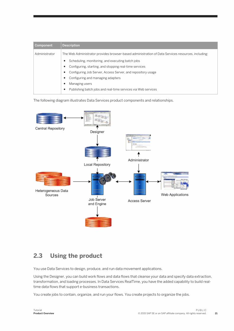
The following diagram illustrates Data Services product components and relationships.
2.3 Using the product
You use Data Services to design, produce, and run data movement applications.
Using the Designer, you can build work flows and data flows that cleanse your data and specify data extraction, transformation, and loading processes. In Data Services RealTime, you have the added capability to build real-time data flows that support e-business transactions.
You create jobs to contain, organize, and run your flows. You create projects to organize the jobs.
TutorialProduct Overview
P U B L I C© 2015 SAP SE or an SAP affiliate company. All rights reserved. 21
Refine and build on your design until you have created a well-tested, production-quality application. In Data Services, you can set applications to run in test mode or on a specific schedule. Using Data Services RealTime, you can run applications in real time so they immediately respond to web-based client requests.
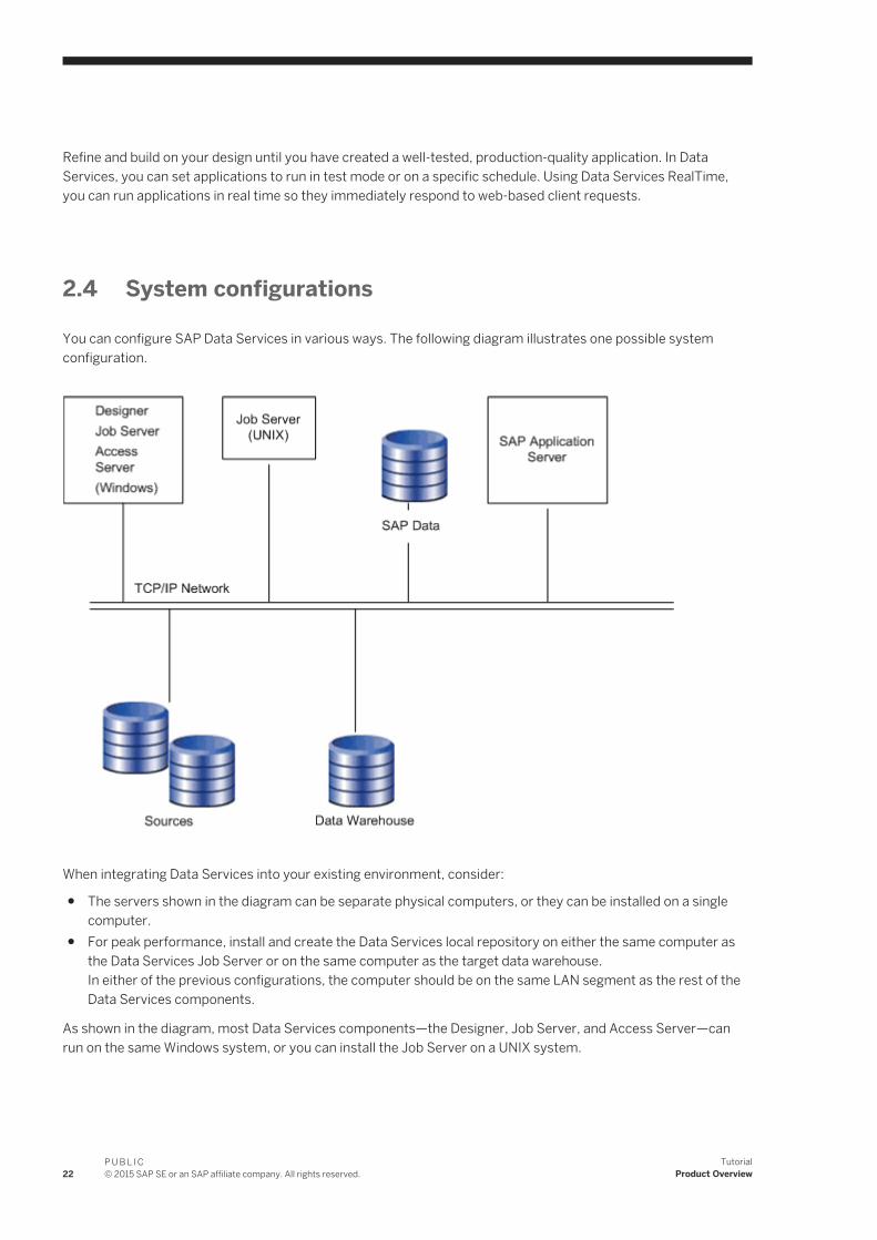
2.4 System configurations
You can configure SAP Data Services in various ways. The following diagram illustrates one possible system configuration.
When integrating Data Services into your existing environment, consider:
● The servers shown in the diagram can be separate physical computers, or they can be installed on a single computer.
● For peak performance, install and create the Data Services local repository on either the same computer as the Data Services Job Server or on the same computer as the target data warehouse.In either of the previous configurations, the computer should be on the same LAN segment as the rest of the Data Services components.
As shown in the diagram, most Data Services components—the Designer, Job Server, and Access Server—can run on the same Windows system, or you can install the Job Server on a UNIX system.
22P U B L I C© 2015 SAP SE or an SAP affiliate company. All rights reserved.
TutorialProduct Overview
2.4.1 Windows implementation
You can configure a Windows system as either a server or a workstation. A large-memory, multiprocessor system is ideal because the multithreading, pipelining, and parallel work flow execution features in Data Services take full advantage of such a system.
You can create your target data warehouse on a database server that may or may not be a separate physical computer.
You can use a shared disk or FTP to transfer data between your source system and the Data Services Job Server.
2.4.2 UNIX implementation
You can install the Data Services Job Server on a UNIX system. You can also configure the Job Server to start automatically when you restart the computer.
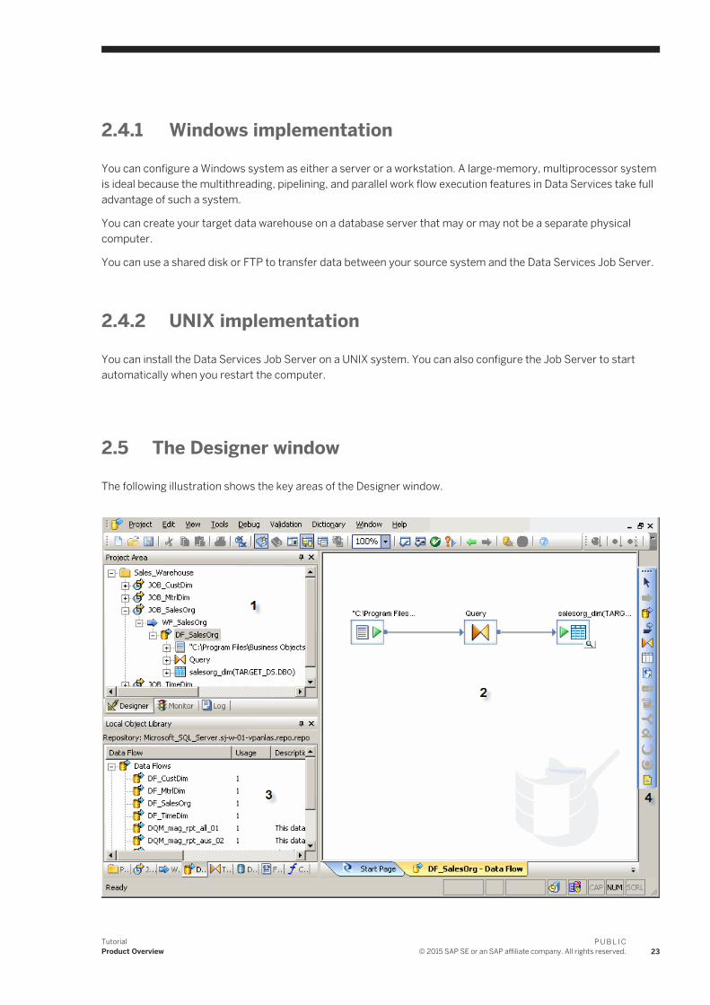
2.5 The Designer window
The following illustration shows the key areas of the Designer window.
TutorialProduct Overview
P U B L I C© 2015 SAP SE or an SAP affiliate company. All rights reserved. 23
The key areas of the Data Services application window are:
1. Project area — Contains the current project (and the job(s) and other objects within it) available to you at a given time. In Data Services, all entities you create, modify, or work with are objects.
2. Workspace — The area of the application window in which you define, display, and modify objects.3. Local object library — Provides access to local repository objects including built-in system objects, such as
transforms and transform configurations, and the objects you build and save, such as jobs and data flows.4. Tool palette — Buttons on the tool palette enable you to add new objects to the workspace.
2.6 Objects
In Data Services, all entities you add, define, modify, or work with are objects. Objects have:
● Options that control the object. For example, to set up a connection to a database, defining the database name would be an option for the connection.
● Properties that describe the object. For example, the name and creation date. Attributes are properties used to locate and organize objects.
● Classes that determine how you create and retrieve the object. You can copy reusable objects from the object library. You cannot copy single-use objects.
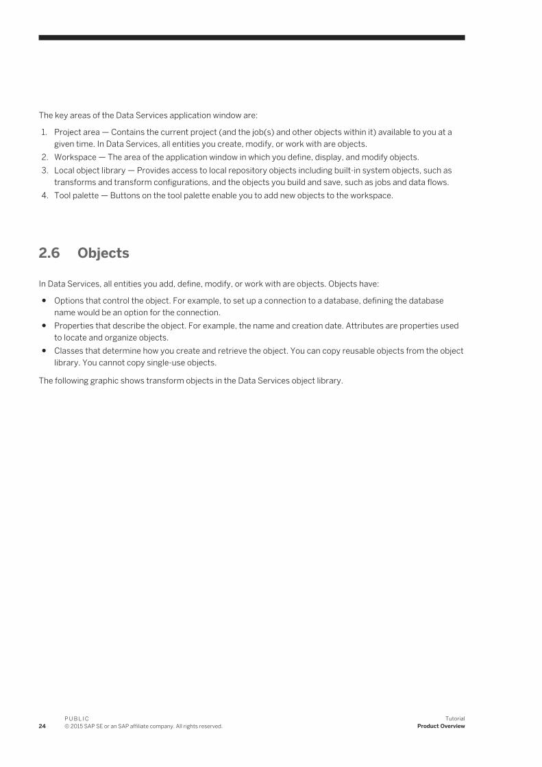
The following graphic shows transform objects in the Data Services object library.
24P U B L I C© 2015 SAP SE or an SAP affiliate company. All rights reserved.
TutorialProduct Overview
When you widen the object library, the name of each object is visible next to its icon. To resize the object library area, click and drag its border until you see the text you want, then release.
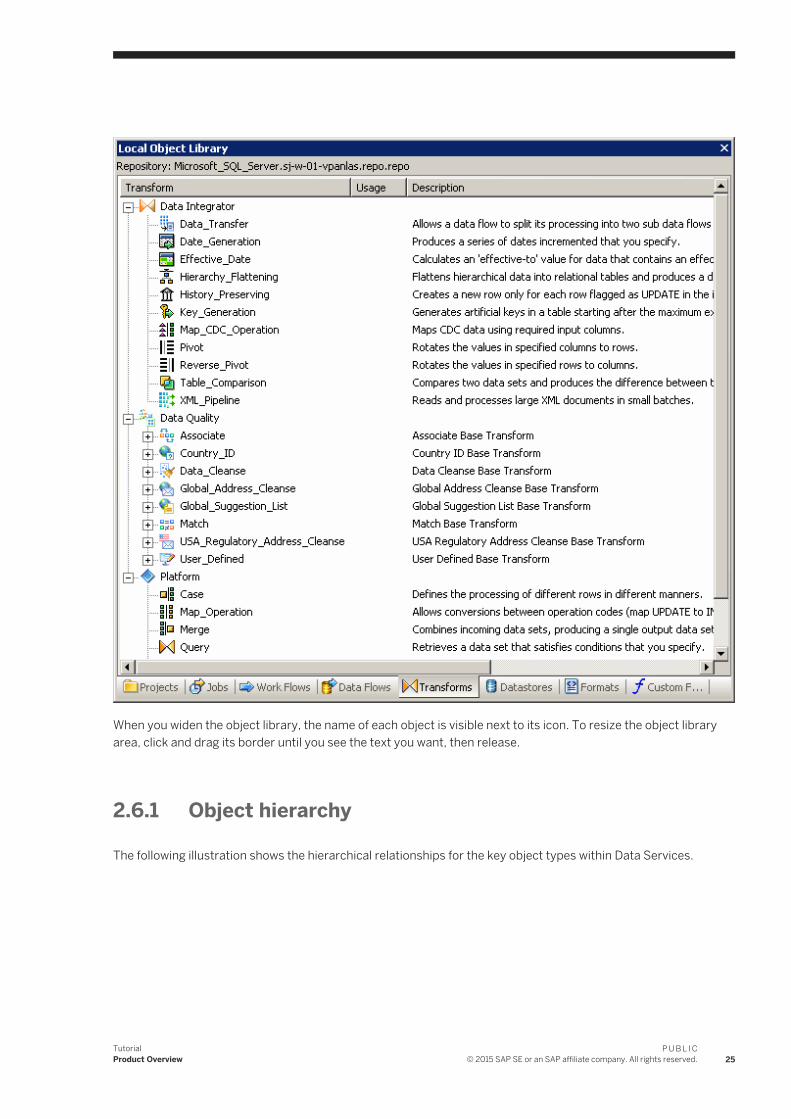
2.6.1 Object hierarchy
The following illustration shows the hierarchical relationships for the key object types within Data Services.
TutorialProduct Overview
P U B L I C© 2015 SAP SE or an SAP affiliate company. All rights reserved. 25

In the repository, the Designer groups objects hierarchically from a project, to jobs, to optional work flows, to data flows. In jobs:
● Work flows define a sequence of processing steps. Work flows and conditionals are optional. A conditional contains work flows, and you can embed a work flow within another work flow.
● Data flows transform data from source(s) to target(s). You can embed a data flow within a work flow or within another data flow.
26P U B L I C© 2015 SAP SE or an SAP affiliate company. All rights reserved.
TutorialProduct Overview
2.6.1.1 Projects and jobs
A project is the highest-level object in the Designer window. Projects provide you with a way to organize the other objects you create in Data Services. Only one project is open at a time (where "open" means "visible in the project area").
A job is the smallest unit of work that you can schedule independently for execution.
2.6.1.2 Work flows and data flows
Jobs are composed of work flows and/or data flows:
● A work flow is the incorporation of several data flows into a coherent flow of work for an entire job.● A data flow is the process by which source data is transformed into target data.
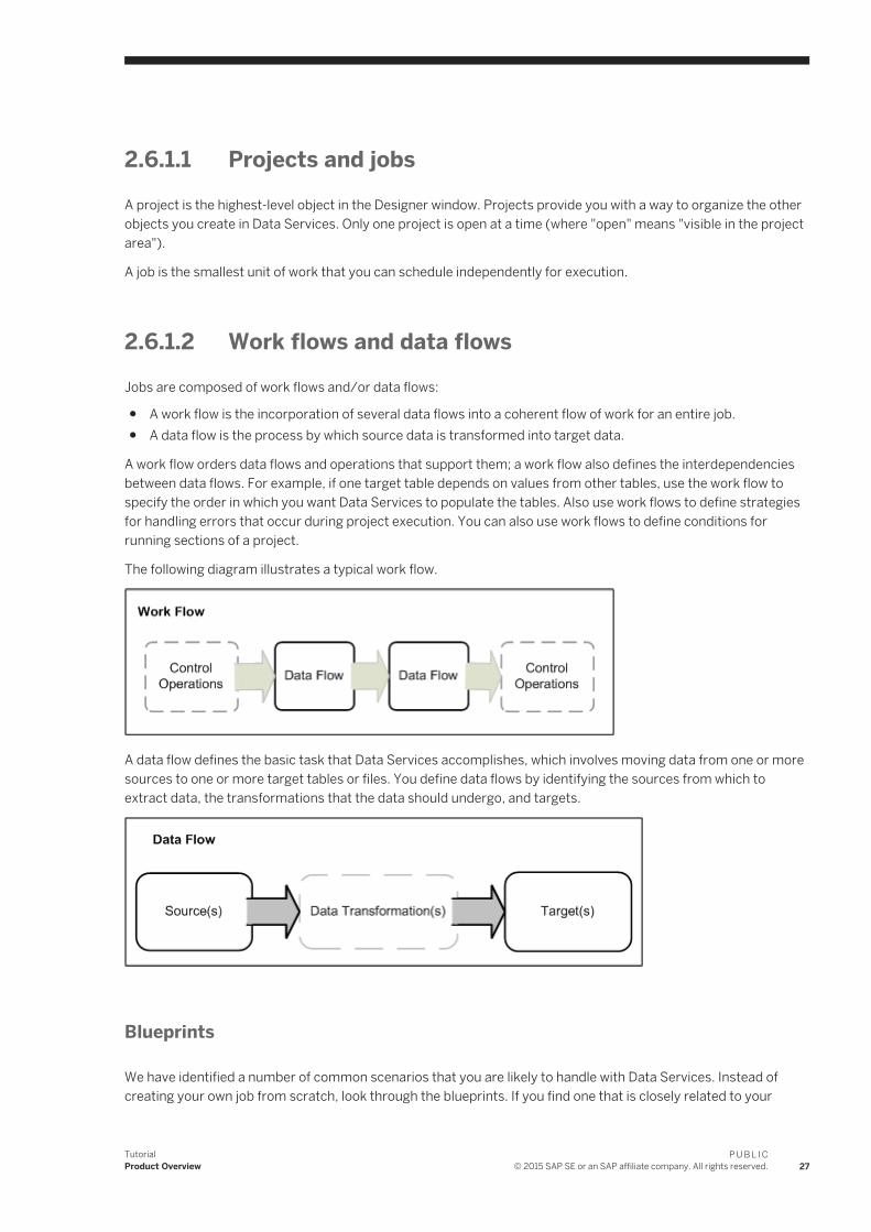
A work flow orders data flows and operations that support them; a work flow also defines the interdependencies between data flows. For example, if one target table depends on values from other tables, use the work flow to specify the order in which you want Data Services to populate the tables. Also use work flows to define strategies for handling errors that occur during project execution. You can also use work flows to define conditions for running sections of a project.
The following diagram illustrates a typical work flow.
A data flow defines the basic task that Data Services accomplishes, which involves moving data from one or more sources to one or more target tables or files. You define data flows by identifying the sources from which to extract data, the transformations that the data should undergo, and targets.
Blueprints
We have identified a number of common scenarios that you are likely to handle with Data Services. Instead of creating your own job from scratch, look through the blueprints. If you find one that is closely related to your
TutorialProduct Overview
P U B L I C© 2015 SAP SE or an SAP affiliate company. All rights reserved. 27
particular business problem, you can simply use the blueprint and tweak the settings in the transforms for your specific needs.
For each scenario, we have included a blueprint that is already set up to solve the business problem in that scenario. Each blueprint contains the necessary Data Services project, jobs, data flows, file formats, sample data, template tables, and custom functions to run the data flows in your environment with only a few modifications.
You can download all of the blueprints or only the blueprints and other content that you find useful from the SAP Community Network. Here, we periodically post new and updated blueprints, custom functions, best practices, white papers, and other Data Services content. You can refer to this site frequently for updated content and use the forums to provide us with any questions or requests you may have. We have also provided the ability for you to upload and share any content that you have developed with the rest of the Data Services development community.
Instructions for downloading and installing the content objects are also located on the SAP Community Network at http://scn.sap.com/docs/DOC-8820 .
2.6.2 Object-naming conventions
Data Services recommends that you follow a consistent naming convention to facilitate object identification. Here are some examples:
Table 9:
Prefix Suffix Object Example
JOB Job JOB_SalesOrg
WF Work flow WF_SalesOrg
DF Data flow DF_Currency
DS Datastore ODS_DS
2.7 New terms
Table 10:
Term Description
Attribute Property that can be used as a constraint for locating objects.
Data flow Contains steps to define how source data becomes target data. Called by a work flow or job.
Datastore Logical channel that connects Data Services to source and target databases.
Job The smallest unit of work that you can schedule independently for execution. A job is a special work flow that cannot be called by another work flow or job.
28P U B L I C© 2015 SAP SE or an SAP affiliate company. All rights reserved.
TutorialProduct Overview

Term Description
Metadata Data that describes the objects maintained by Data Services.
Object Any project, job, work flow, data flow, datastore, file format, message, custom function, transform, or transform configurations created, modified, or used in Data Services.
Object library Part of the Designer interface that represents a "window" into the local repository and provides access to reusable objects.
Option A choice in a dialog box that controls how an object functions.
Project Logical grouping of related jobs. The Designer can open only one project at a time.
Property Characteristic used to define the state, appearance, or value of an object; for example, the name of the object or the date it was created.
Repository A database that stores Designer predefined system objects and user-defined objects including source and target metadata and transformation rules. Can be local or central (shared).
Source Table, file, or legacy system from which Data Services reads data.
Target Table or file to which Data Services loads data.
Work flow Contains steps to define the order of job execution. Calls a data flow to manipulate data.
2.8 Section summary and what to do next
This section has given you a short overview of the Data Services product and terminology. For more information about these topics, see the Administrator Guide and the Designer Guide.
TutorialProduct Overview
P U B L I C© 2015 SAP SE or an SAP affiliate company. All rights reserved. 29
3 Defining Source and Target Metadata
In this section you will set up logical connections between Data Services, a flat-file source, and a target data warehouse. You will also create and import objects into the local repository. Storing connection metadata in the repository enables you to work within Data Services to manage tables that are stored in various environments.
3.1 Logging in to the Designer
When you log in to the Designer, you must log in as a user defined in the Central Management Server (CMS).
1. From the Start menu, click Programs SAP Data Services 4.2 Data Services Designer .
As Data Services starts, a login screen appears.2. Enter your user credentials for the CMS.
Table 11:
Option Description
System Specify the server name and optionally the port for the CMS.
User name Specify the user name to use to log into CMS.
Password Specify the password to use to log into the CMS.
Authentication Specify the authentication type used by the CMS.
3. Click Log On.The software attempts to connect to the CMS using the specified information. When you log in successfully, the list of local repositories that are available to you is displayed.
4. Select the repository you want to use.5. Click OK to log in using the selected repository.
In the next section you will define datastores (connections) for your source and target.
3.2 Defining a datastore
Datastores:
● Provide a logical channel (connection) to a database● Must be specified for each source and target database● Are used to import metadata for source and target databases into the repository.
30P U B L I C© 2015 SAP SE or an SAP affiliate company. All rights reserved.
TutorialDefining Source and Target Metadata

● Are used by Data Services to read data from source tables and load data to target tables
The databases to which Data Services datastores can connect include:
● Oracle● IBM DB2● Microsoft SQL Server● Sybase ASE● Sybase IQ● ODBC
Metadata consists of:
● Database tables○ Table name○ Column names○ Column data types○ Primary key columns○ Table attributes
● RDBMS functions● Application-specific data structures
Connection metadata is defined in the object library as datastores (for tables) and file formats (for flat files).
The next task describes how to define datastores using the Designer. Note that while you are designating the datastores as sources or targets, datastores only function as connections. You will define the actual source and target objects when you define data flows later in the tutorial.
3.2.1 Defining a datastore for the source (ODS) database
1. From the Datastores tab of the object library, right-click in the blank area and click New.The Create New Datastore window opens. A example for the Oracle environment appears as follows:
TutorialDefining Source and Target Metadata
P U B L I C© 2015 SAP SE or an SAP affiliate company. All rights reserved. 31
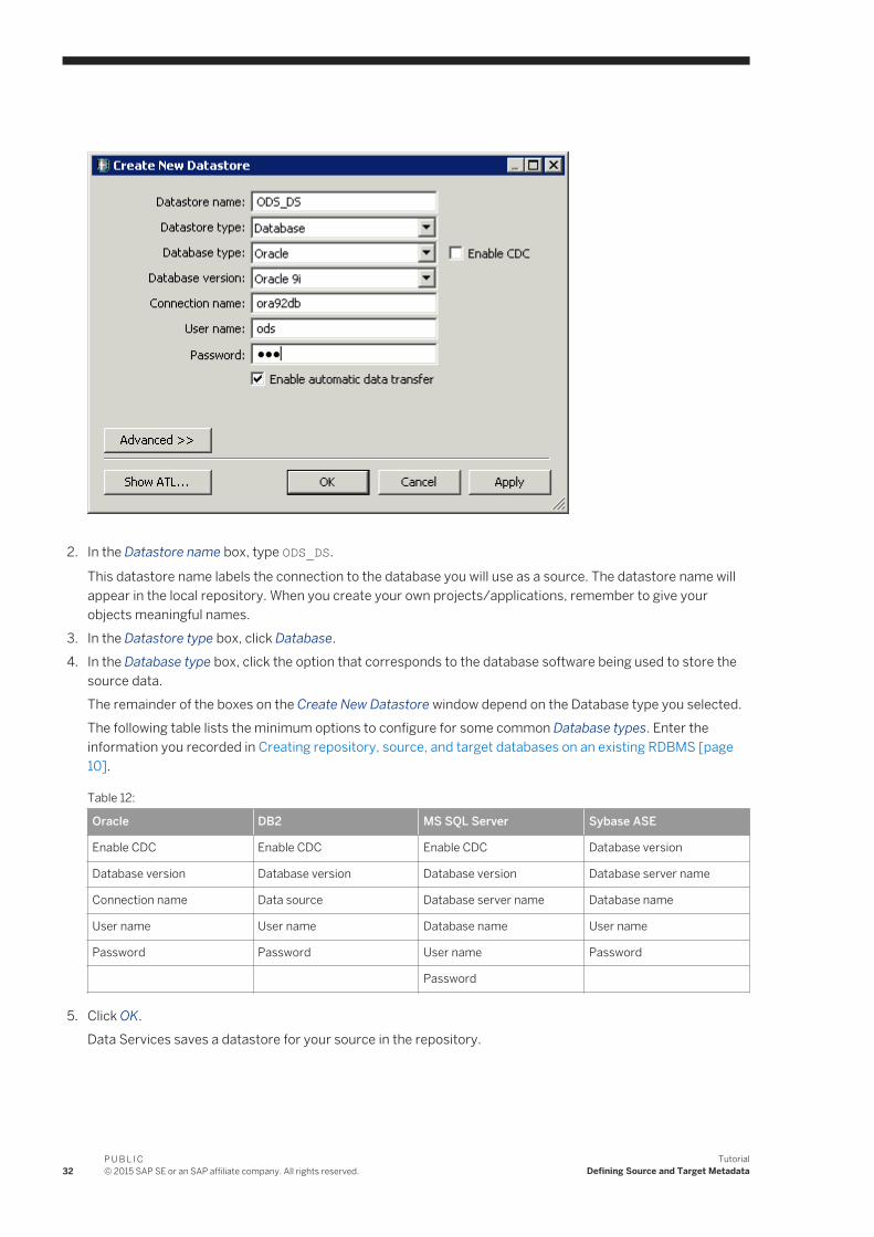
2. In the Datastore name box, type ODS_DS.
This datastore name labels the connection to the database you will use as a source. The datastore name will appear in the local repository. When you create your own projects/applications, remember to give your objects meaningful names.
3. In the Datastore type box, click Database.4. In the Database type box, click the option that corresponds to the database software being used to store the
source data.The remainder of the boxes on the Create New Datastore window depend on the Database type you selected.The following table lists the minimum options to configure for some common Database types. Enter the information you recorded in Creating repository, source, and target databases on an existing RDBMS [page 10].
Table 12:
Oracle DB2 MS SQL Server Sybase ASE
Enable CDC Enable CDC Enable CDC Database version
Database version Database version Database version Database server name
Connection name Data source Database server name Database name
User name User name Database name User name
Password Password User name Password
Password
5. Click OK.Data Services saves a datastore for your source in the repository.
32P U B L I C© 2015 SAP SE or an SAP affiliate company. All rights reserved.
TutorialDefining Source and Target Metadata
3.2.2 Defining a datastore for the target database
Define a datastore for the target database using the same procedure as for the source (ODS) database.
1. Use Target_DS for the datastore name.
2. Use the information you recorded in Creating repository, source, and target databases on an existing RDBMS [page 10].
3.3 Importing metadata
With Data Services, you can import metadata for individual tables using a datastore. You can import metadata by:
● Browsing● Name● Searching
The following procedure describes how to import by browsing.
3.3.1 Importing metadata for ODS source tables
1. In the Datastores tab, right-click the ODS_DS datastore and click Open.
The names of all the tables in the database defined by the datastore named ODS_DS display in a window in the workspace.
2. Move the cursor over the right edge of the Metadata column heading until it changes to a resize cursor.3. Double-click the column separator to automatically resize the column.4. Import the following tables by right-clicking each table name and clicking Import. Alternatively, because the
tables are grouped together, click the first name, Shift-click the last, and import them together. (Use Ctrl-click for nonconsecutive entries.)○ ods.ods_customer○ ods.ods_material○ ods.ods_salesorder○ ods.ods_salesitem○ ods.ods_delivery○ ods.ods_employee○ ods.ods_region
Data Services imports the metadata for each table into the local repository.
NoteIn Microsoft SQL Server, the owner prefix might be dbo instead of ods.
5. In the object library on the Datastores tab, under ODS_DS expand the Tables node and verify the tables have been imported into the repository.
TutorialDefining Source and Target Metadata
P U B L I C© 2015 SAP SE or an SAP affiliate company. All rights reserved. 33
3.3.2 Importing metadata for target tables
1. Open the Target_DS datastore.2. Import the following tables by right-clicking each table name and clicking Import. Alternatively, use Ctrl-click
and import them together○ target.status_table○ target.cust_dim○ target.employee_dim○ target.mtrl_dim○ target.sales_fact○ target.salesorg_dim○ target.time_dim○ target.CDC_time
Data Services imports the metadata for each table into the local repository.
NoteIn Microsoft SQL Server, the owner prefix might be dbo instead of target.
3. In the object library on the Datastores tab, under Target_DS expand the Tables node and verify the tables have been imported into the repository.
3.4 Defining a file format
If the source or target RDBMS includes data stored in flat files, you must define file formats in Data Services. File formats are a set of properties that describe the structure of a flat file.
Data Services includes a file format editor. Use it to define flat file formats. The editor supports delimited and fixed-width formats.
You can specify file formats for one file or a group of files. You can define flat files from scratch or by importing and modifying an existing flat file. Either way, Data Services saves a connection to the file or file group.
NoteData Services also includes a file format (Transport_Format) that you can use to read flat files in SAP applications.
In the next section, you will use a flat file as your source data. Therefore, you must create a file format and connection to the file now.
1. In the object library, click the Formats tab, right-click in a blank area of the object library, and click NewFile Format .The file format editor opens.
2. Under General, leave Type as Delimited. Change the Name to Format_SalesOrg.
34P U B L I C© 2015 SAP SE or an SAP affiliate company. All rights reserved.
TutorialDefining Source and Target Metadata
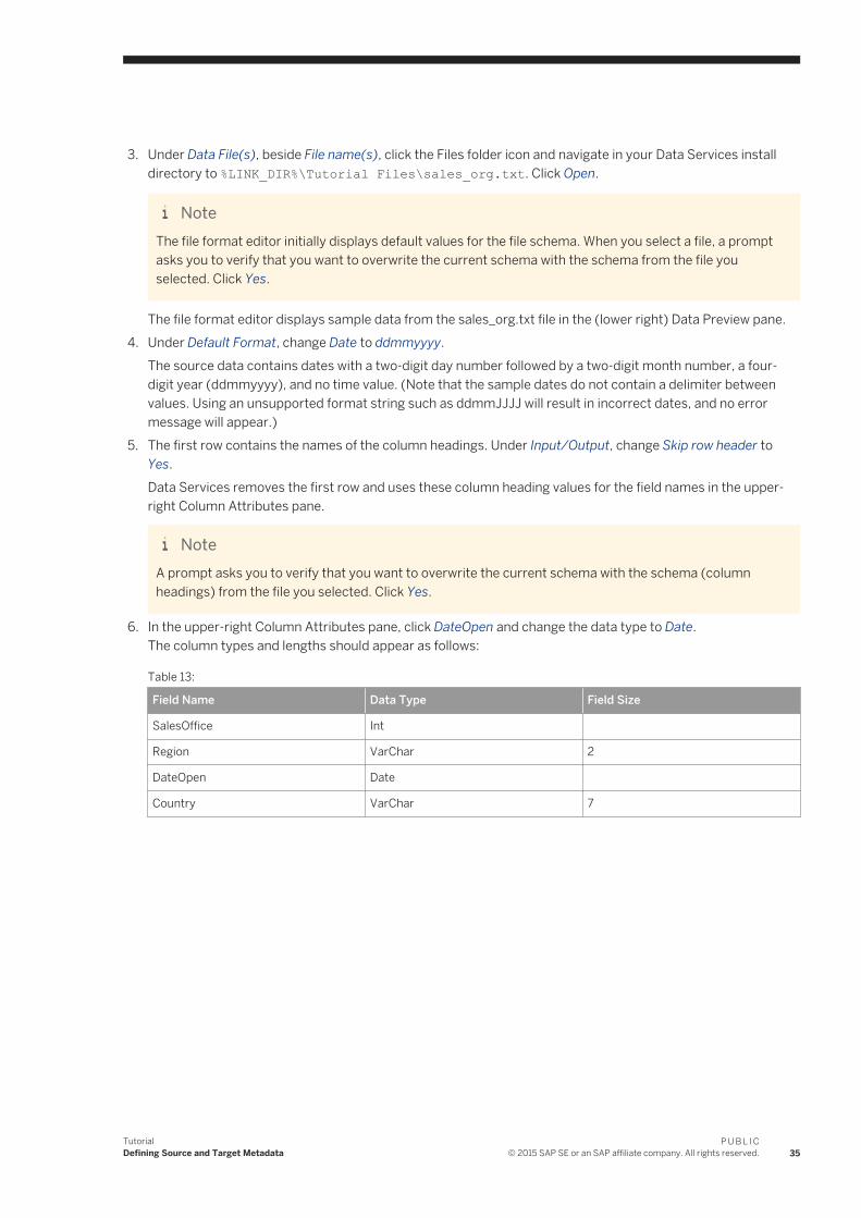
3. Under Data File(s), beside File name(s), click the Files folder icon and navigate in your Data Services install directory to %LINK_DIR%\Tutorial Files\sales_org.txt. Click Open.
NoteThe file format editor initially displays default values for the file schema. When you select a file, a prompt asks you to verify that you want to overwrite the current schema with the schema from the file you selected. Click Yes.
The file format editor displays sample data from the sales_org.txt file in the (lower right) Data Preview pane.4. Under Default Format, change Date to ddmmyyyy.
The source data contains dates with a two-digit day number followed by a two-digit month number, a four-digit year (ddmmyyyy), and no time value. (Note that the sample dates do not contain a delimiter between values. Using an unsupported format string such as ddmmJJJJ will result in incorrect dates, and no error message will appear.)
5. The first row contains the names of the column headings. Under Input/Output, change Skip row header to Yes.Data Services removes the first row and uses these column heading values for the field names in the upper-right Column Attributes pane.
NoteA prompt asks you to verify that you want to overwrite the current schema with the schema (column headings) from the file you selected. Click Yes.
6. In the upper-right Column Attributes pane, click DateOpen and change the data type to Date.The column types and lengths should appear as follows:
Table 13:
Field Name Data Type Field Size
SalesOffice Int
Region VarChar 2
DateOpen Date
Country VarChar 7
TutorialDefining Source and Target Metadata
P U B L I C© 2015 SAP SE or an SAP affiliate company. All rights reserved. 35

7. Click Save & Close.
3.5 New terms
The terms examined in this section included:
Table 14:
Term Meaning
Datastore Connection from Data Services to tables in source or target databases. Stored as an object in the repository.
36P U B L I C© 2015 SAP SE or an SAP affiliate company. All rights reserved.
TutorialDefining Source and Target Metadata
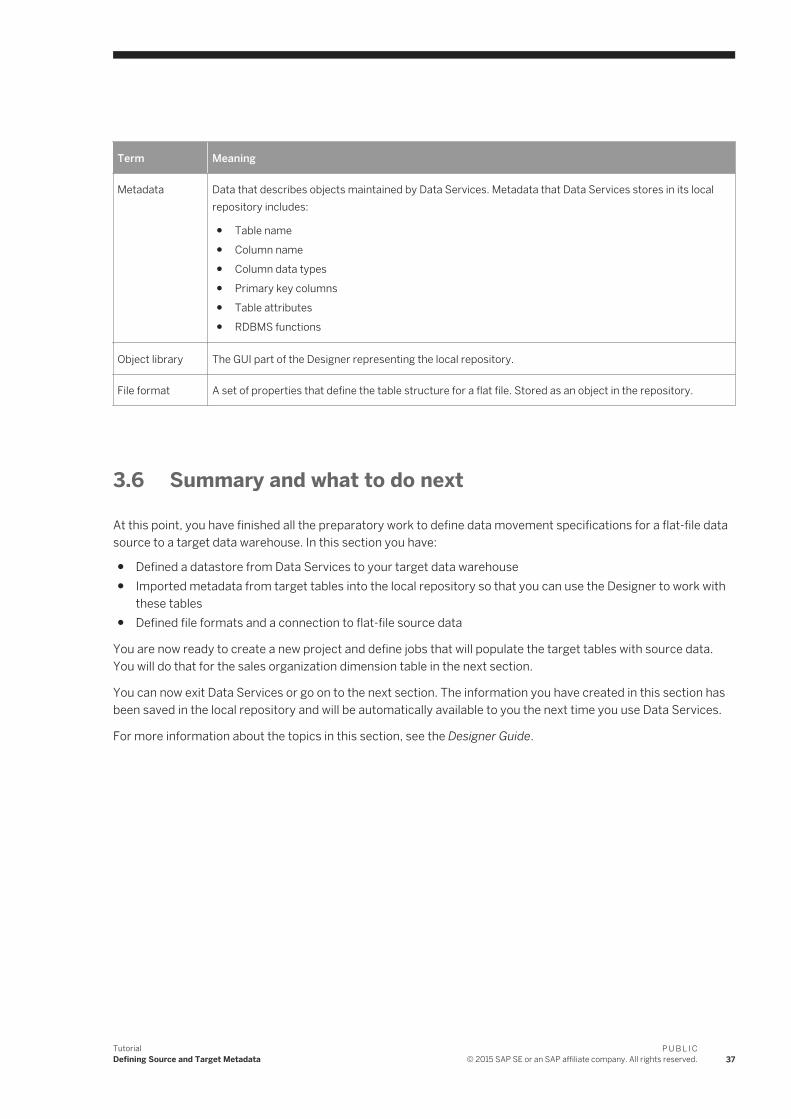
Term Meaning
Metadata Data that describes objects maintained by Data Services. Metadata that Data Services stores in its local repository includes:
● Table name● Column name● Column data types● Primary key columns● Table attributes● RDBMS functions
Object library The GUI part of the Designer representing the local repository.
File format A set of properties that define the table structure for a flat file. Stored as an object in the repository.
3.6 Summary and what to do next
At this point, you have finished all the preparatory work to define data movement specifications for a flat-file data source to a target data warehouse. In this section you have:
● Defined a datastore from Data Services to your target data warehouse● Imported metadata from target tables into the local repository so that you can use the Designer to work with
these tables● Defined file formats and a connection to flat-file source data
You are now ready to create a new project and define jobs that will populate the target tables with source data. You will do that for the sales organization dimension table in the next section.
You can now exit Data Services or go on to the next section. The information you have created in this section has been saved in the local repository and will be automatically available to you the next time you use Data Services.
For more information about the topics in this section, see the Designer Guide.
TutorialDefining Source and Target Metadata
P U B L I C© 2015 SAP SE or an SAP affiliate company. All rights reserved. 37

4 Populating the SalesOrg Dimension from a Flat File
In this section, you will populate the sales organization dimension table in your target data warehouse with data from a flat file called Format_SalesOrg.
4.1 Objects and their hierarchical relationships
Everything in Data Services is an object. The key objects involved in data movement activities (like projects, jobs, work flows, and data flows) display in the Designer project area according to their relationship in the object hierarchy.
The following figure shows a display of the types of objects you will be creating while you are working in this section.
38P U B L I C© 2015 SAP SE or an SAP affiliate company. All rights reserved.
TutorialPopulating the SalesOrg Dimension from a Flat File
1. Project2. Job3. Work flow4. Data flow
Object hierarchies are displayed in the project area of the Designer.
4.2 Adding a new project
Projects group and organize related objects. Projects display in the project area of the Designer and can contain any number of jobs, work flows, and data flows.
1. In the Designer, from the Project menu click New Project .2. Name the project Class_Exercises.
3. Click Create.
The project name appears as the only object in the project area of the Designer.
Next, you will define the job that will be used to extract the information from the flat-file source.
4.3 Adding a job
A job is a reusable object. It is also the second level in the project hierarchy. It contains work flows (which contain the order of steps to be executed) and data flows (which contain data movement instructions). You can execute jobs manually or as scheduled.
In this exercise you will define a job called JOB_SalesOrg.
1. Right-click in the project area and click New Batch Job.2. Right-click the new job and click Rename. Alternatively, left-click the job twice (slowly) to make the name
editable.3. Type JOB_SalesOrg.
4. Left-click or press Enter.
The job appears in the project hierarchy under Class_Exercises and in the project tab of the object library.
4.4 About work flows
A work flow is a reusable object. It executes only within a Job. Use work flows to:
● Call data flows● Call another work flow
TutorialPopulating the SalesOrg Dimension from a Flat File
P U B L I C© 2015 SAP SE or an SAP affiliate company. All rights reserved. 39

● Define the order of steps to be executed in your job● Pass parameters to and from data flows● Define conditions for executing sections of the project● Specify how to handle errors that occur during execution
Work flows are optional.
The Data Services objects you can use to create work flows appear on the tool palette:
Table 15:
Button Component Programming Analogy
Work flow Procedure
Data Flow Declarative SQL select statement
Script Subset of lines in a procedure
Conditional If/then/else logic
While Loop A sequence of steps that repeats as long as a condition is true
Try Try block indicator
Catch Try block terminator and exception handler
Annotation Description of a job, work flow, data flow, or a diagram in a workspace
4.4.1 Adding a work flow
1. With JOB_SalesOrg selected in the project area, click the work flow button on the tool palette. 2. Click the blank workspace area.
A work flow icon appears in the workspace. The work flow also appears in the project area on the left under the job name (expand the job to view).
NoteYou can place a work flow anywhere in the workspace, but because flows are best viewed from left to right and top to bottom, place it near the top left corner.
3. Change the name of the work flow to WF_SalesOrg.
40P U B L I C© 2015 SAP SE or an SAP affiliate company. All rights reserved.
TutorialPopulating the SalesOrg Dimension from a Flat File
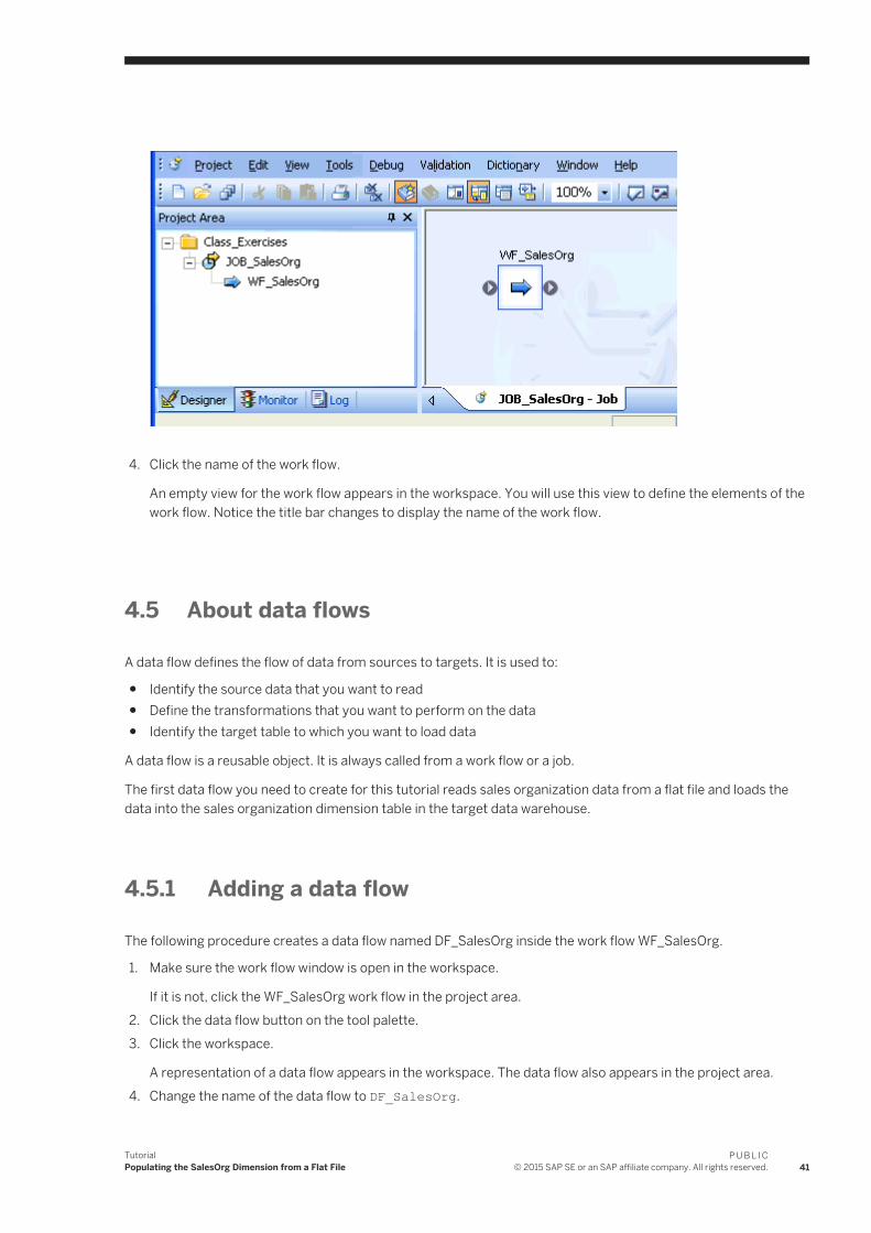
4. Click the name of the work flow.
An empty view for the work flow appears in the workspace. You will use this view to define the elements of the work flow. Notice the title bar changes to display the name of the work flow.
4.5 About data flows
A data flow defines the flow of data from sources to targets. It is used to:
● Identify the source data that you want to read● Define the transformations that you want to perform on the data● Identify the target table to which you want to load data
A data flow is a reusable object. It is always called from a work flow or a job.
The first data flow you need to create for this tutorial reads sales organization data from a flat file and loads the data into the sales organization dimension table in the target data warehouse.
4.5.1 Adding a data flow
The following procedure creates a data flow named DF_SalesOrg inside the work flow WF_SalesOrg.
1. Make sure the work flow window is open in the workspace.
If it is not, click the WF_SalesOrg work flow in the project area.2. Click the data flow button on the tool palette.3. Click the workspace.
A representation of a data flow appears in the workspace. The data flow also appears in the project area.4. Change the name of the data flow to DF_SalesOrg.
TutorialPopulating the SalesOrg Dimension from a Flat File
P U B L I C© 2015 SAP SE or an SAP affiliate company. All rights reserved. 41

Notice the project, job, work flow, and data flow objects display in hierarchical form in both the project area and the object library. To navigate to these levels, click their names in the project area.
1—Data flow in the workspace
2—Data flow in the project area
3—Data flow in the local object library5. Click the data flow name.
A definition area for the data flow appears in the workspace. This area will be used to define the data flow as described in the next section.
42P U B L I C© 2015 SAP SE or an SAP affiliate company. All rights reserved.
TutorialPopulating the SalesOrg Dimension from a Flat File

4.5.2 Defining the data flow
Inside the data flow, you must specify the instructions to transform source data into the form you want for the target table. In this case, you will define the data flow instructions for building the sales organization dimension table using the following objects:
● An object representing the source file● An object defining a query transform (or query). A query transform maps columns from source to target. With
a query transform, you can:○ Select row sets○ Create joins○ Group and order by data values○ Create data set filters○ Execute functions
● An object representing the target table into which the data loads
The next three exercises guide you through the steps necessary to define a data flow's content:
1. Add objects to the data flow.2. Connect them in the order that data will flow through them.3. Define the query that maps the source columns to the target columns.
4.5.2.1 Adding objects to a data flow
1. Verify the DF_SalesOrg data flow is open in the workspace. In the object library, click the Formats tab.
2. The source for this data flow will be the flat file Format_SalesOrg. Click and drag the Format_SalesOrg object to the workspace.
3. Drop the Format_SalesOrg object on the left side of the workspace to leave room for more objects on the right.
4. Click Make Source from the shortcut menu that appears when you drop the object.
5. Click the query button on the tool palette. 6. Click to the right of the source file in the workspace.7. In the object library, click the Datastores tab and expand the datastore named Target_DS.8. The target for this data flow will be the table SALESORG_DIM. Click and drag the SALESORG_DIM object to
the workspace and drop it to the right of the query.9. Click Make Target from the shortcut menu that appears when you drop the table. Data Services creates a
table with the same schema as the query output schema.
All the elements necessary to create the sales organization dimension table are now in the workspace. In the next section, you will connect the steps in the correct order.
TutorialPopulating the SalesOrg Dimension from a Flat File
P U B L I C© 2015 SAP SE or an SAP affiliate company. All rights reserved. 43
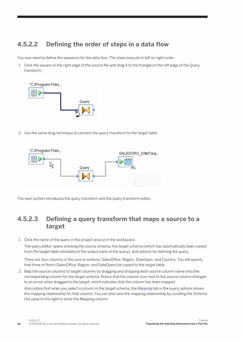
4.5.2.2 Defining the order of steps in a data flow
You now need to define the sequence for the data flow. The steps execute in left-to-right order.
1. Click the square on the right edge of the source file and drag it to the triangle on the left edge of the Query transform.
2. Use the same drag technique to connect the query transform to the target table.
The next section introduces the query transform and the query transform editor.
4.5.2.3 Defining a query transform that maps a source to a target
1. Click the name of the query in the project area or in the workspace.The query editor opens showing the source schema, the target schema (which has automatically been copied from the target table metadata to the output pane of the query), and options for defining the query.
There are four columns in the source schema: SalesOffice, Region, DateOpen, and Country. You will specify that three of them (SalesOffice, Region, and DateOpen) be copied to the target table.
2. Map the source columns to target columns by dragging and dropping each source column name onto the corresponding column for the target schema. Notice that the column icon next to the source column changes to an arrow when dragged to the target, which indicates that the column has been mapped.Also notice that when you select a column in the target schema, the Mapping tab in the query options shows the mapping relationship for that column. You can also view the mapping relationship by scrolling the Schema Out pane to the right to show the Mapping column.
44P U B L I C© 2015 SAP SE or an SAP affiliate company. All rights reserved.
TutorialPopulating the SalesOrg Dimension from a Flat File
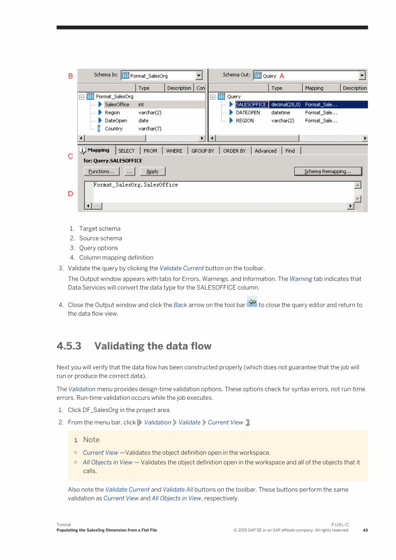
1. Target schema2. Source schema3. Query options4. Column mapping definition
3. Validate the query by clicking the Validate Current button on the toolbar.The Output window appears with tabs for Errors, Warnings, and Information. The Warning tab indicates that Data Services will convert the data type for the SALESOFFICE column.
4. Close the Output window and click the Back arrow on the tool bar to close the query editor and return to the data flow view.
4.5.3 Validating the data flow
Next you will verify that the data flow has been constructed properly (which does not guarantee that the job will run or produce the correct data).
The Validation menu provides design-time validation options. These options check for syntax errors, not run-time errors. Run-time validation occurs while the job executes.
1. Click DF_SalesOrg in the project area.
2. From the menu bar, click Validation Validate Current View .
Note○ Current View —Validates the object definition open in the workspace.○ All Objects in View — Validates the object definition open in the workspace and all of the objects that it
calls.
Also note the Validate Current and Validate All buttons on the toolbar. These buttons perform the same validation as Current View and All Objects in View, respectively.
TutorialPopulating the SalesOrg Dimension from a Flat File
P U B L I C© 2015 SAP SE or an SAP affiliate company. All rights reserved. 45

Data Services displays the Output dialog box with the Warning tab indicating that Data Services will convert the data type for the SALESOFFICE column.
If the Output window displays any errors, correct them before proceeding.
Related Information
Executing the job [page 46]
4.5.4 Addressing errors
1. Right-click an error message and click View.
Data Services displays the Error Message window in which you can read the expanded error message text.2. Double-click the error message to open the editor of the object containing the error.
NoteWarning messages do not prohibit job execution.
You have validated the data flow and completed the description of the data movement for the sales organization dimension table.
4.6 Saving the project
You can save the steps you have completed and close Data Services at any time.
To save all objects in a project, from the Project menu click Save All. Or, when you close a project or exit the program, Data Services lists all recently changed items and prompts you to save them.
To save work displayed only in the active object workspace, from the Project menu click Save.
4.7 Executing the job
Now you will execute the job you have just created.
First verify that your job server is running by looking at the job server icon at the bottom right of the Designer window. Move the pointer over the icon to see the Job Server name, machine name, and port number in the status area. If the job server is not running, the icon will have a red X on it.
46P U B L I C© 2015 SAP SE or an SAP affiliate company. All rights reserved.
TutorialPopulating the SalesOrg Dimension from a Flat File

1. Select the job name in the project area, in this case JOB_SalesOrg.
2. Right-click and click Execute.If you have changed any objects and not yet saved them, Data Services prompts you to save your work. Click OK.
Data Services validates the job again before running it. If there are syntax errors, review the error messages and return to the design and validate the effected steps of the job. Also review any warning messages before dismissing them.
If the job validates properly, the Execution Properties dialog box appears. These properties include execution parameters and options to set traces and global variables.
TutorialPopulating the SalesOrg Dimension from a Flat File
P U B L I C© 2015 SAP SE or an SAP affiliate company. All rights reserved. 47
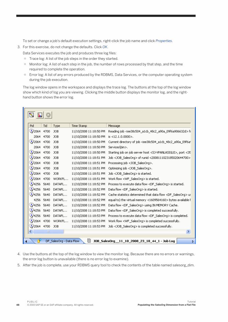
To set or change a job's default execution settings, right-click the job name and click Properties.3. For this exercise, do not change the defaults. Click OK.
Data Services executes the job and produces three log files:○ Trace log: A list of the job steps in the order they started.○ Monitor log: A list of each step in the job, the number of rows processed by that step, and the time
required to complete the operation.○ Error log: A list of any errors produced by the RDBMS, Data Services, or the computer operating system
during the job execution.
The log window opens in the workspace and displays the trace log. The buttons at the top of the log window show which kind of log you are viewing. Clicking the middle button displays the monitor log, and the right-hand button shows the error log.
4. Use the buttons at the top of the log window to view the monitor log. Because there are no errors or warnings,
the error log button is unavailable (there is no error log to examine).5. After the job is complete, use your RDBMS query tool to check the contents of the table named salesorg_dim.
48P U B L I C© 2015 SAP SE or an SAP affiliate company. All rights reserved.
TutorialPopulating the SalesOrg Dimension from a Flat File
4.8 About deleting objects
Deleting a job or other object from the project area does not delete it from the object library. The object still exists in any other projects to which it has been assigned. Deleting an object from the object library, however, deletes all occurrences of the object.
4.9 New terms
The terms introduced in this section included:
Table 16:
Term Meaning
Query options Tabs in the query editor that defines properties of the output schema
Query A Data Services transform object
Schema A description of the data layout of a table
Transform A Data Services object that defines data transformation
4.10 Summary and what to do next
You have now defined and run your first data movement job—a job that populates the sales organization dimension table in the target data warehouse.
The next section introduces you to time dimension tables. In that exercise you will populate the time dimension table with some simple time attributes:
● Year number● Month number● Business quarter
The next section also introduces you to the Date_Generation transform.
TutorialPopulating the SalesOrg Dimension from a Flat File
P U B L I C© 2015 SAP SE or an SAP affiliate company. All rights reserved. 49

5 Populating the Time Dimension Using a Transform
The exercise in this section builds and populates a time dimension table. Time dimension tables contain date/time-related attributes such as season, holiday period, fiscal quarter, and others that are not directly ascertainable from traditional SQL style date/time data types.
The time dimension table in this example is simple in that it contains only the year number, month number, and business quarter as time attributes. It uses a Julian date as a primary key.
The tasks in this section include:
● Retrieving the project [page 50]● Adding the job and data flow [page 51]● Defining the time dimension data flow [page 51]● Saving and executing the job [page 53]
5.1 Retrieving the project
If you have closed Data Services, reopen the Class_Exercises project.
50P U B L I C© 2015 SAP SE or an SAP affiliate company. All rights reserved.
TutorialPopulating the Time Dimension Using a Transform

5.1.1 Opening the Class_Exercises project
1. Start Data Services.2. Log in to your repository.
3. Click Project Open .4. Click Class_Exercises.5. Click OK.
5.2 Adding the job and data flow
As you have done in the previous exercise, you will begin with creating a job that contains a data flow. A work flow is not necessary for this job; you will be calling the data flow directly from the job.
1. Add a job named JOB_TimeDim that will load data into the time dimension table.
For a reminder about how to create a job, see Adding a job [page 39].2. Open JOB_TimeDim and create a data flow object named DF_TimeDim. (Do not create a work flow this time.)
5.3 Defining the time dimension data flow
The data flow instructions for populating a time dimension table consist of the following objects:
● A Date_Generation transform as a source.● A query to produce column values from the generated dates such as what day the date falls on, the quarter
it's in, and so on.● A target table into which the time dimension data loads.
5.3.1 Specifying the components of the time data flow
1. Open the data flow named DF_TimeDim.
2. In the object library, click the Transforms tab. 3. Expand the Data Integrator folder and click the Date_Generation transform.
Transforms are predefined Data Services objects.4. Drag the transform icon into the workspace and drop it on the left side of the workspace to leave room for
more objects to the right.
5. Click the query button on the tool palette.
TutorialPopulating the Time Dimension Using a Transform
P U B L I C© 2015 SAP SE or an SAP affiliate company. All rights reserved. 51

6. Click in the workspace to the right of the Date_Generation transform.7. In the object library for the datastore named Target_DS, drag the table named TIME_DIM into the workspace
and drop it to the right of the query.8. Click Make Target from the shortcut menu.
All the objects you need to create a time dimension table are now available in the workspace. Next you will connect the objects in the order they need to be executed.
5.3.2 Defining the flow of data
1. Click the square on the right edge of the Date_Generation transform and drag to the triangle on the left edge of the query.
2. Use the same drag technique to connect the query to the TIME_DIM target.
The connections indicate the flow of data through these instructions.
The following sections define the details of each step of the data flow.
5.3.3 Defining the output of the Date_Generation transform
The Date_Generation transform produces a column of dates for a range and increment you specify.
1. Click the name of the Date_Generation transform to open the transform editor.2. Enter these values in the editor columns:
Table 17:
Start Date 2002.01.01
End Date 2008.12.31
Increment daily
3. Click the Back arrow in the tool bar to close the transform editor and return to the data flow.
The date column serves as the input to the query. The query allows you to apply functions to the input columns and map those columns to an internal data set (the query output).
52P U B L I C© 2015 SAP SE or an SAP affiliate company. All rights reserved.
TutorialPopulating the Time Dimension Using a Transform

5.3.4 Defining the output of the query
1. Click the query icon in the project area.The query editor shows an input schema with a single column, the output schema copied from the target, and options for the query.
2. Map the generated date to the NATIVEDATE column by dragging the DI_GENERATED_DATE column from the input schema to the NATIVEDATE output column.Alternatively, you can drag and drop the DI_GENERATED_DATE column from the source pane into the mapping expression. The column name DI_GENERATED_DATE will be qualified with the name of the Date_Generation transform; for example, Date_Generation_1.DI_GENERATED_DATE.
3. Click each column name in the target schema (one by one) and define the mapping for the column using the following table. The mapping definition applies to the column selected in the target schema. Type the mapping expression directly on the Mapping tab.Alternatively, click the Functions button to open the Function editor and add functions to the mapping definition that way.
These are the mapping expressions and function descriptions for the rest of the columns:
Table 18:
Column name Mapping Function description
Date_ID julian(di_generated_date) Use the JULIAN function to set the Julian date for that date value.
YearNum to_char(di_generated_date,'yyyy')
Use the TO_CHAR function to select only the year out of the date value. Enclose yyyy in single quotes.
MonthNum month(di_generated_date) Use the MONTH function to set the month number for that date value.
BusQuarter quarter(di_generated_date) Use the QUARTER function to set the quarter for that date value.
You might notice that the tutorial simplifies the quarter calculation. For the purposes of the tutorial, assume that the business year is the same as the calendar year.
4. Click the Back arrow on the tool bar.
These columns are now the input schema for the TIME_DIM table.
This completes the data-movement description for the time dimension table.
5.4 Saving and executing the job
Save the project. For a reminder of how to save a project, see Saving the project [page 46].
Execute the job JOB_TimeDim. After the job runs, check the contents of the TIME_DIM table with a query tool for the RDBMS on which your target data warehouse is stored.
TutorialPopulating the Time Dimension Using a Transform
P U B L I C© 2015 SAP SE or an SAP affiliate company. All rights reserved. 53
5.5 Summary and what to do next
You have now populated two tables in the sales data warehouse:
● Sales Org dimension (from a flat file)● Time dimension, which consists of a date generation transform and a query
In the next section, you will extract data to populate the customer dimension table.
At this point, you can exit Data Services or go on to the next exercise.
For more information about the topics covered in this section, see the Designer Guide.
54P U B L I C© 2015 SAP SE or an SAP affiliate company. All rights reserved.
TutorialPopulating the Time Dimension Using a Transform
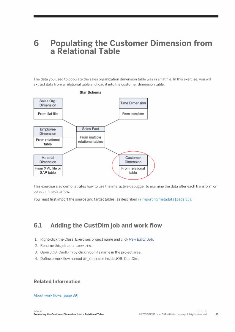
6 Populating the Customer Dimension from a Relational Table
The data you used to populate the sales organization dimension table was in a flat file. In this exercise, you will extract data from a relational table and load it into the customer dimension table.
This exercise also demonstrates how to use the interactive debugger to examine the data after each transform or object in the data flow.
You must first import the source and target tables, as described in Importing metadata [page 33].
6.1 Adding the CustDim job and work flow
1. Right-click the Class_Exercises project name and click New Batch Job.2. Rename this job JOB_CustDim.
3. Open JOB_CustDim by clicking on its name in the project area.4. Define a work flow named WF_CustDim inside JOB_CustDim.
Related Information
About work flows [page 39]
TutorialPopulating the Customer Dimension from a Relational Table
P U B L I C© 2015 SAP SE or an SAP affiliate company. All rights reserved. 55

6.2 Adding the CustDim data flow
1. Verify the WF_CustDim work flow window is open in the workspace.If not, click the WF_CustDim work flow name in the project area (or in the workspace if visible)
2. Add a data flow to the work flow definition.3. Rename the data flow DF_CustDim.
4. Click the name of the data flow to open the data flow definition.
6.3 Defining the CustDim data flow
The data flow instructions for building the dimension table will consist of the following objects:
● The source table● A query● The target table into which the customer dimension data loads
6.3.1 Bringing the objects into the data flow
1. Verify the DF_CustDim data flow is open in the workspace.2. In the object library, view the list of tables in the ODS_DS datastore. Drag and drop the CUSTOMER table to
the left side of the workspace and click Make Source.3. Click the query icon on the tool palette and click to the right of the table to place the query in the workspace.
4. In the object library, from the list of tables for the Target_DS datastore, drag and drop the CUST_DIM table to the right of the query and click Make Target.
5. Connect the icons to indicate the flow of data, as shown.
56P U B L I C© 2015 SAP SE or an SAP affiliate company. All rights reserved.
TutorialPopulating the Customer Dimension from a Relational Table

6.3.2 Defining the query
1. In the workspace, click the name of the query to open the query editor.2. Remap the following source columns to the target schema, leaving the names and data types as they are in
the target.
Table 19:
Column Data type Description
Cust_ID varchar(10) Customer number
Cust_classf varchar(2) Customer classification
Name1 varchar(35) Customer name
Address varchar(35) Address
City varchar(35) City
Region_ID varchar(2) Region
Zip varchar(10) Postal code
(Do not map Cust_Timestamp.)
NoteIn Microsoft SQL Server and Sybase ASE, you must specify the columns in the order shown in the table.
3. Click the Back arrow in the icon bar to return to the data flow.
6.4 Validating the CustDim data flow
Next you will verify that the data flow has been constructed properly.
From the menu bar, click Validation Validate All Objects in View .
If your design contains syntax errors, a dialog box appears with a message describing the error. Warning messages usually do not affect proper execution of the job.
If your data flow contains no errors, the following message appears:
Validate: No Errors Found
6.5 Executing the CustDim job
Just as you executed the job named JOB_SalesOrg in the previous exercise, execute the job named JOB_CustDim:
TutorialPopulating the Customer Dimension from a Relational Table
P U B L I C© 2015 SAP SE or an SAP affiliate company. All rights reserved. 57

1. In the project area, right-click the job name and click Execute.
A prompt appears to save your work:
2. Click OK.3. Click OK on the Execution Properties window.4. After the job completes, ensure there are no error or warning messages.5. To view the captured sample data, in the project area click the data flow to open it in the workspace. Click the
magnifying glass on an object to view the data.
Or, use a query tool to check the contents of the CUST_DIM table.
6.6 Using the interactive debugger
The Designer includes an interactive debugger that allows you to examine and modify data row by row by placing filters and breakpoints on lines in a data flow diagram. The debugger allows you to examine what happens to the data after each transform or object in the flow.
A debug filter functions as a simple query transform with a WHERE clause. Use a filter to reduce a data set in a debug job execution. A breakpoint is the location where a debug job execution pauses and returns control to you.
This exercise demonstrates how to set a breakpoint and view data in debug mode.
6.6.1 Setting a breakpoint in a data flow
1. Click the name of the DF_CustDim data flow to open its definition.2. Right-click the line between the source table and the query and click Set Filter/Breakpoint.3. In the Breakpoint pane, select the Set check box and click OK.
58P U B L I C© 2015 SAP SE or an SAP affiliate company. All rights reserved.
TutorialPopulating the Customer Dimension from a Relational Table

6.6.2 Using the interactive debugger
1. In the project area, right-click Job_CustDim and click Start debug.If prompted to save your work, click OK.
The Debug Properties window opens.2. Click OK.3. To process the next row, from the Debug menu click Get Next Row.
The next row replaces the existing row in the right View Data pane. To see all rows, select the All check box.4. To stop the debug mode, from the Debug menu, click Stop Debug, or click the Stop Debug button on the
toolbar.
TutorialPopulating the Customer Dimension from a Relational Table
P U B L I C© 2015 SAP SE or an SAP affiliate company. All rights reserved. 59

Note that when you open the interactive debugger, in addition to the View Data panes below the work space, the Designer displays additional panes:
1. View data panes2. Call Stack pane3. Trace pane4. Debug Variables pane
The left View Data pane shows the data in the CUSTOMER source table, and the right pane shows one row at a time (the default) that has passed to the query.
You can set a condition in a breakpoint to search for specific rows. For example, you might want to stop the data flow when the debugger reaches a row with a Region_ID value of 2.
6.6.3 Setting a breakpoint condition
1. Open the breakpoint dialog box by double-clicking the breakpoint.2. Click under the Column heading. Click the down arrow to display a drop-down list of columns. Click
CUSTOMER.REGION_ID.3. Click under the Operator heading. Click the down arrow to display a drop-down list of operators. Click = .
60P U B L I C© 2015 SAP SE or an SAP affiliate company. All rights reserved.
TutorialPopulating the Customer Dimension from a Relational Table

4. Click under the Value heading and type 2.
5. Click OK.6. Right-click the job name and click Start debug.
The debugger stops after processing the first row with a Region_ID of 2, as the right View Data pane shows.7. To stop the debug mode, from the Debug menu, click Stop Debug, or click the Stop Debug button on the
toolbar.
6.7 Summary and what to do next
You have now populated three tables in the sample data warehouse:
● Sales organization dimension (from a flat file)● Time dimension (using Date Generation transform)● Customer dimension (from a relational table)
In the next section, you will populate the Material dimension table.
For more information about the topics covered in this section, see the Designer Guide.
TutorialPopulating the Customer Dimension from a Relational Table
P U B L I C© 2015 SAP SE or an SAP affiliate company. All rights reserved. 61

7 Populating the Material Dimension from an XML File
In this section, you will extract data from an XML file (mtrl.xml) that contains nested data and flatten selected elements from it to populate the denormalized material dimension table. You will also import a DTD for the XML file.
The tasks in this section include:
● Adding MtrlDim job, work and data flows [page 62]● Importing a document type definition [page 63]● Defining the MtrlDim data flow [page 63]● Validating that the MtrlDim data flow has been constructed properly [page 65]● Executing the MtrlDim job [page 66]● Leveraging the XML_Pipeline [page 66]
7.1 Adding MtrlDim job, work and data flows
1. Add a new job and name it JOB_MtrlDim. (For details, see Adding the CustDim job and work flow [page 55].)
2. Add a work flow and name it WF_MtrlDim. (For details, see Adding the CustDim job and work flow [page 55].)
3. Click the WF_MtrlDim name to open it in the workspace.
4. Add a data flow to the work flow definition and name it DF_MtrlDim.
62P U B L I C© 2015 SAP SE or an SAP affiliate company. All rights reserved.
TutorialPopulating the Material Dimension from an XML File
7.2 Importing a document type definition
Import the document type definition (DTD) mtrl.dtd as described in the following procedure.
1. Open the object library and go to the Formats tab.2. Right-click DTDs and click New. The Import DTD Format dialog box opens.3. In the DTD definition name box, name the DTD Mtrl_List.4. For the File name, click Browse to navigate to the mtrl.dtd file in your Data Services directory at \Tutorial Files
\mtrl.dtd and open it.5. For file type, keep the default DTD option.6. In the Root element name list, click MTRL_MASTER_LIST.7. Click OK.
7.3 Defining the MtrlDim data flow
The data flow components for building a material dimension table will consist of the following objects:
● The source XML file● A query to map the nested source schema to the flat target schema● The target table into which the material dimension data loads
7.3.1 Adding the objects to the data flow
1. Click the name of the data flow to open the data flow definition.2. In the object library on the file formats tab, expand DTDs if it is not already expanded.3. Drag the Mtrl_List file into the DF_MtrlDim definition workspace, drop it on the left side, and click Make XML
File Source.4. Click the Mtrl_List name in the workspace to configure it.5. On the Source tab, in the XML file list, click <Select file>. Navigate to the mtrl.xml file at \Data Services
\Tutorial Files\mtrl.xml. Click Open to import the mtrl.xml file.
6. Select Enable validation to enable comparison of the incoming data to the stored DTD format.7. Click the back arrow to return to the data flow.8. Click the query transform icon in the tool palette, click to the right of the table in the workspace, and name the
query qryunnest.9. From the list of tables in the object library for the Target_DS datastore, drag the MTRL_DIM table to the
workspace, drop it to the right of qryunnest, and click Make Target.10. Connect the icons to indicate the flow of data from the source XML file through the query to the target table.
TutorialPopulating the Material Dimension from an XML File
P U B L I C© 2015 SAP SE or an SAP affiliate company. All rights reserved. 63
7.3.2 Defining the details of qryunnest
1. Click on the query name to open the query editor. Notice the nested structure of the source in the Schema In pane.
2. Try dragging an individual column across to one of the columns in the output pane. Notice that you cannot map a nested column to a column in the flat target schema. This exercise unnests the input schema to flatten it to fit the target table.
3. Notice the differences in column names and data types between the input and output schemas. (Use the scroll bar if necessary to view data types).
4. To capture the required output schema, select the five columns in the output pane, right-click and Cut them to the clipboard.
NoteYou cut these columns, rather than delete them, to capture the correct column names and data types from the target schema. You will later paste these columns into the appropriate nested context from the source to avoid editing the source column names and data types.
5. From the Schema In pane, drag the MTRL_MASTER schema to the Schema Out pane.6. In the project area, click the MTRL.DIM target table to view its editor. Notice that the output structure from
the preceding query (the Schema In, shown in the left pane) contains more information than required by the desired output schema and requires flattening to fit the target table.
7. In the project area, click qryunnest to view its editor. In the output structure (right pane), right-click the MTRL_MASTER schema and choose Make Current to make it available for editing.
8. Select all the columns from MTRL_ID down to and including the HAZMAT_IND nested schema and delete them.
9. Right-click the MTRL_MASTER schema and paste the columns you cut from the target table.10. Remap the MTRL_ID, MTRL_TYPE, IND_SECTOR, and MRTL_GROUP columns to the corresponding columns
in the output schema.11. The DESCR target column needs to be mapped to SHORT_TEXT, which is located in a nested schema.
a. To capture its column name and data type, select DESCR and Cut it to the clipboard.b. In the Schema Out pane, right-click the TEXT schema, and click Make Current.c. In the Schema Out pane, right-click the LANGUAGE column, select Paste, and select Insert Below to place
the DESCR column at the same level as the SHORT_TEXT column.d. From the Schema In pane, map the SHORT_TEXT column to the DESCR column.
12. In the Schema Out pane, select LANGUAGE, SHORT_TEXT, and TEXT_nt_1. Right-click and Delete these columns and nested schema from the TEXT schema.
13. In the project area, click the MTRL_DIM target table to again view its schema. Notice that the input schema is not flat and therefore will not produce the flat schema required by the target.
14. In the project area, click qryunnest to again view the query editor. In the output schema, right-click the TEXT schema and click Unnest. The table icon changes to one with an arrow.
15. View the target table schema again. Notice that the input schema still has two levels versus one in the target.16. Return to the query editor. Right-click MTRL_MASTER in the output schema and click Make Current, then
right-click again and click Unnest.
64P U B L I C© 2015 SAP SE or an SAP affiliate company. All rights reserved.
TutorialPopulating the Material Dimension from an XML File

17. View the target table schema to see that the schemas now match.18. From the Project menu, click Save All.
7.4 Validating that the MtrlDim data flow has been constructed properly
Next you will verify that the data flow has been constructed properly.
1. In the project area, click the data flow.
2. From the Validation menu, click Validate All Objects in View .
You should see warning messages indicating that data types will be converted (which is acceptable because you chose to preserve the date types from the output schema). Review the warning messages and continue.
If your design contains syntax errors, a dialog box appears with a message describing the error. Address all errors before continuing.
If you get the error message: "The flat loader...cannot be connected to NRDM," right-click the error message and click Go to error, which opens the editor for the object in question. In this case, the source schema is still nested. Return to the qryunnest editor and unnest the output schema(s).
The next section describes how to execute the job.
TutorialPopulating the Material Dimension from an XML File
P U B L I C© 2015 SAP SE or an SAP affiliate company. All rights reserved. 65

7.5 Executing the MtrlDim job
1. In the project area, right-click JOB_MtrlDim and click Execute.2. If prompted to save your work, click OK.3. In the Execution Properties dialog box, click OK.4. After the job completes, ensure there are no error or warning messages.5. To view the captured sample data, in the project area select the data flow to open it in the workspace. Click
the magnifying glass on the target MTRL.DIM table to view its six rows.
Or, use a query tool to check the contents of the MTRL.DIM table.
The next section describes an alternate way to capture XML data.
7.6 Leveraging the XML_Pipeline
When you extract data from an XML file to load into a target data warehouse, you usually obtain only parts of the XML file. The Query transform does partial extraction (as the previous exercise shows), and it does much more because it has many of the clauses of a SQL SELECT statement.
The main purpose of the XML_Pipeline transform is to extract parts of your XML file. Because the XML_Pipeline transform focuses on this partial extraction, it utilizes memory more efficiently and performs better than the Query transform for this purpose.
● The XML_Pipeline transform uses less memory because it processes each instance of a repeatable schema within the XML file, rather than building the whole XML structure first.
● The XML_Pipeline transform continually releases and reuses memory to steadily flow XML data through the transform.
You can use the XML_Pipeline transform as an alternate way to build the Material dimension table. The data flow components for this alternate way will consist of the following objects:
● The source XML file● An XML_Pipeline transform to obtain a repeatable portion of the nested source schema● A query to map the output of the XML_Pipeline transform to the flat target schema● The target table into which the material dimension data loads
7.6.1 Setting up a job and data flow that uses the XML_Pipeline transform
1. Add a new job and name it JOB_Mtrl_Pipe.
2. Add a new work flow job and name it WF_Mtrl_Pipe.
3. Add a data flow to the work flow definition and name it DF_Mtrl_Pipe.
4. Click the name of the data flow to open the data flow definition.
66P U B L I C© 2015 SAP SE or an SAP affiliate company. All rights reserved.
TutorialPopulating the Material Dimension from an XML File

5. In the object library on the Formats tab, expand DTDs if it is not already expanded.6. Drag the Mtrl_List file into the DF_Mtrl_Pipe definition workspace, drop it on the left side, and click Make XML
File Source.7. Click the Mtrl_List name in the workspace to configure it.8. On the Source tab, in the XML file list, click <Select file>. Navigate to the mtrl.xml file at \Data Services
\Tutorial Files\mtrl.xml. Click Open to import the mtrl.xml file.
9. Select Enable Validation to enable comparison of the incoming data to the stored DTD format.10. Click the back arrow to return to the data flow.11. In the object library on the Transforms tab, expand the Data Integrator transforms.12. Drag the XML_Pipeline transform into the DF_Mtrl_Pipe definition workspace, drop it to the right of Mtrl_List
source.13. In the object library on the Transforms tab, expand the Platform transforms.14. Drag the Query transform into the workspace, drop it to the right of XML_Pipeline , and name the query
Query_Pipeline.15. From the list of tables in the object library for the Target_DS datastore, drag the MTRL_DIM table to the
workspace, drop it to the right of Query_Pipeline, and click Make Target.16. Connect the icons to indicate the flow of data from the source XML file through the XML_Pipeline and
Query_Pipeline transforms to the target table.
7.6.2 Defining the details of XML_Pipeline and Query_Pipeline
1. Click XML_Pipeline to open the transform editor. Notice the nested structure of the source in the Schema In pane.
2. Drag the MTRL_ID, MTRL_TYPE, IND_SECTOR, MRTL_GROUP, and SHORT_TEXT columns to the output schema.
NoteUnlike the Query transform, the XML_Pipeline transform allows you to map a nested column directly to a flat target.
3. Return to the data flow (either click the back arrow or click DF_Mtrl_Pipe in the project area).4. Click Query_Pipeline to open the query editor.
TutorialPopulating the Material Dimension from an XML File
P U B L I C© 2015 SAP SE or an SAP affiliate company. All rights reserved. 67

5. Drag each Schema In column to the corresponding columns in the output schema. If you are remapping the fields, choose Remap Column from the menu that appears. The Remap Column option preserves the name and data type in Schema Out.
Table 20:
Schema In column name Schema Out column name
MTRL_ID MTRL_ID
MTRL_TYPE MTRL_TYP
IND_SECTOR IND_SECTOR
MTRL_GROUP MTRL_GRP
SHORT_TEXT DESCR
6. In the project area, click the MTRL_DIM table to open the target editor. In the Options tab, select the Delete data from table before loading option.
7. In the project area, click DF_MTRL_Pipe to return to the data flow.
8. From the Validation menu, click Validate All Objects in View .
You should see warning messages indicating that data types will be converted (which is acceptable because you chose to preserve the data types from the output schema). Review the warning messages and continue.
9. In the project area, right-click JOB_Mtrl_Pipe and click Execute.10. If prompted to save your work, click OK.11. In the Execution Properties dialog box, click OK.12. After the job completes, ensure there are no error or warning messages.13. To view the captured sample data, in the project area select the data flow to open it in the workspace. Click
the magnifying glass on the target MTRL.DIM table to view its six rows.Or, use a query tool to check the contents of the MTRL.DIM table.
7.7 Summary and what to do next
You have now populated four tables in the sample data warehouse:
● Sales organization dimension from a flat file● Time dimension using the Date Generation transform● Customer dimension from a relational table● Material dimension from a nested XML file
In the next section you will populate the sales fact table.
Related Information
Designer Guide: Nested Data
68P U B L I C© 2015 SAP SE or an SAP affiliate company. All rights reserved.
TutorialPopulating the Material Dimension from an XML File

Reference Guide: Transforms
TutorialPopulating the Material Dimension from an XML File
P U B L I C© 2015 SAP SE or an SAP affiliate company. All rights reserved. 69
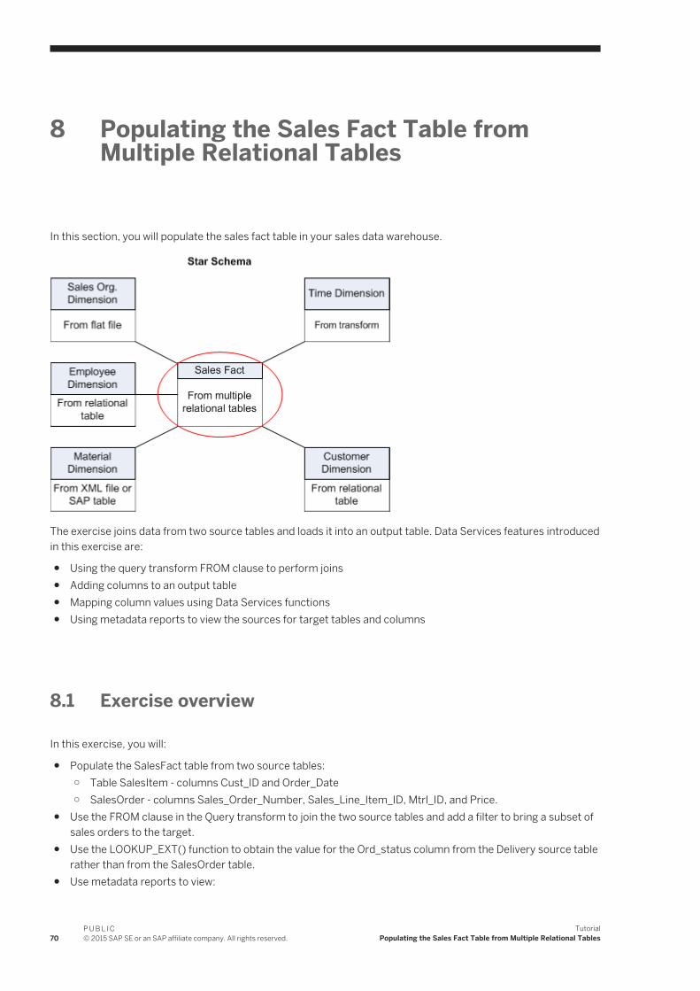
8 Populating the Sales Fact Table from Multiple Relational Tables
In this section, you will populate the sales fact table in your sales data warehouse.
The exercise joins data from two source tables and loads it into an output table. Data Services features introduced in this exercise are:
● Using the query transform FROM clause to perform joins● Adding columns to an output table● Mapping column values using Data Services functions● Using metadata reports to view the sources for target tables and columns
8.1 Exercise overview
In this exercise, you will:
● Populate the SalesFact table from two source tables:○ Table SalesItem - columns Cust_ID and Order_Date○ SalesOrder - columns Sales_Order_Number, Sales_Line_Item_ID, Mtrl_ID, and Price.
● Use the FROM clause in the Query transform to join the two source tables and add a filter to bring a subset of sales orders to the target.
● Use the LOOKUP_EXT() function to obtain the value for the Ord_status column from the Delivery source table rather than from the SalesOrder table.
● Use metadata reports to view:
70P U B L I C© 2015 SAP SE or an SAP affiliate company. All rights reserved.
TutorialPopulating the Sales Fact Table from Multiple Relational Tables
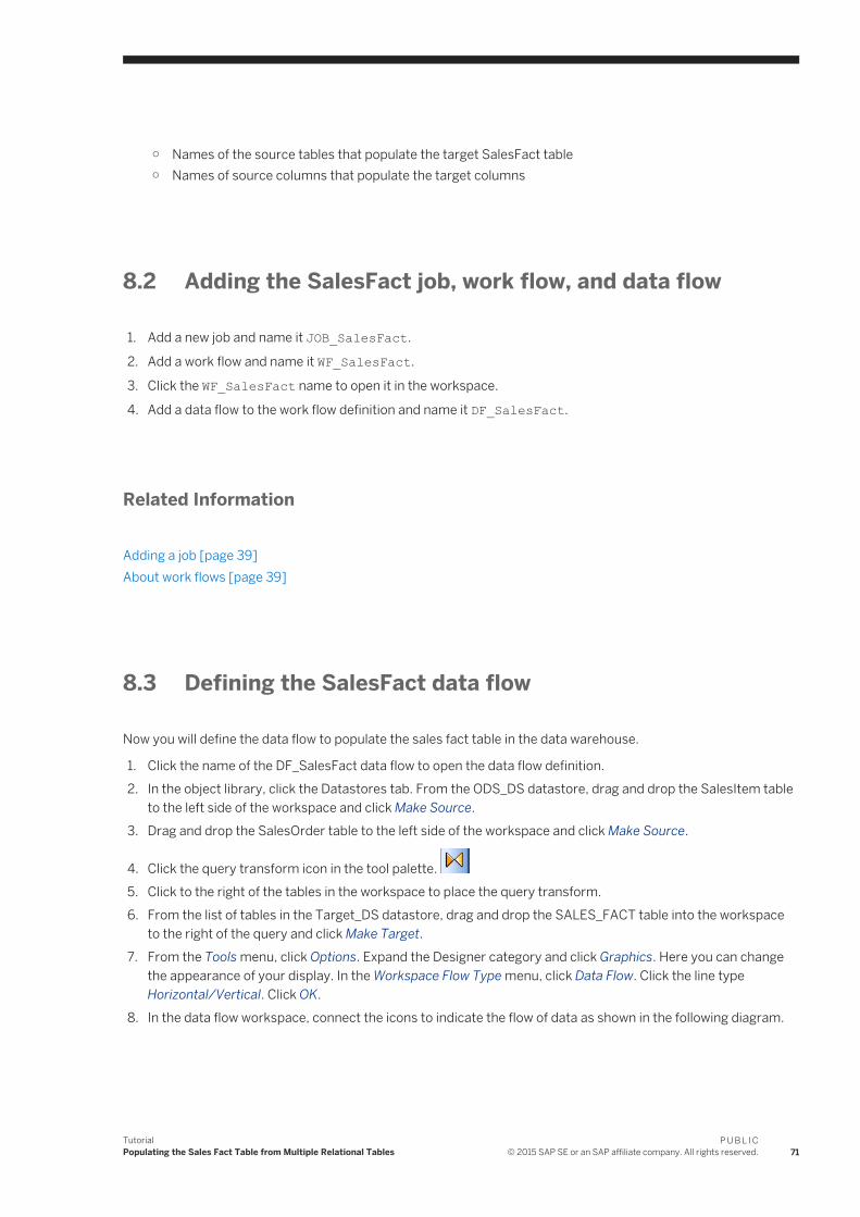
○ Names of the source tables that populate the target SalesFact table○ Names of source columns that populate the target columns
8.2 Adding the SalesFact job, work flow, and data flow
1. Add a new job and name it JOB_SalesFact.
2. Add a work flow and name it WF_SalesFact.
3. Click the WF_SalesFact name to open it in the workspace.
4. Add a data flow to the work flow definition and name it DF_SalesFact.
Related Information
Adding a job [page 39]About work flows [page 39]
8.3 Defining the SalesFact data flow
Now you will define the data flow to populate the sales fact table in the data warehouse.
1. Click the name of the DF_SalesFact data flow to open the data flow definition.2. In the object library, click the Datastores tab. From the ODS_DS datastore, drag and drop the SalesItem table
to the left side of the workspace and click Make Source.3. Drag and drop the SalesOrder table to the left side of the workspace and click Make Source.
4. Click the query transform icon in the tool palette. 5. Click to the right of the tables in the workspace to place the query transform.6. From the list of tables in the Target_DS datastore, drag and drop the SALES_FACT table into the workspace
to the right of the query and click Make Target.7. From the Tools menu, click Options. Expand the Designer category and click Graphics. Here you can change
the appearance of your display. In the Workspace Flow Type menu, click Data Flow. Click the line type Horizontal/Vertical. Click OK.
8. In the data flow workspace, connect the icons to indicate the flow of data as shown in the following diagram.
TutorialPopulating the Sales Fact Table from Multiple Relational Tables
P U B L I C© 2015 SAP SE or an SAP affiliate company. All rights reserved. 71

8.4 Defining the details of the Query transform
1. Open the query editor.2. In the FROM tab, in the Join pairs area, select ODS_SALESORDER from the Left drop-down list.3. Select ODS_SALESITEM from the Right drop-down list.
The relationship between the SalesItem and SalesOrder sales tables is defined by the common column Sales_Order_Number. The Join option generates a join expression based on primary/foreign keys and column names.
The resulting relationship appears in the From clause text box:
SALESITEM.SALES_ORDER_NUMBER = SALESORDER.SALES_ORDER_NUMBER
4. Click the smart editor icon. 5. In the Smart Editor, type the following text. Use all uppercase, as shown. This statement filters the sales
orders by date and brings one year's sales orders into the target. Also note that as you type the function names, a pop-up window prompts you with options. To select an option that is highlighted, press Enter (or double-click any option in the list).
AND ODS_SALESORDER.ORDER_DATE >= to_date('2007.01.01','yyyy.mm.dd') AND ODS_SALESORDER.ORDER_DATE <= to_date('2007.12.31','yyyy.mm.dd') 6. Click OK.7. Map the following source columns to output columns. Remember that to map the contents of a column,
select the column in the source schema and drag it to the target schema.
Table 21:
Source table Column Data type Description Target column (in order)
SALESORDER CUST_ID varchar(10) Customer ID CUST_ID
72P U B L I C© 2015 SAP SE or an SAP affiliate company. All rights reserved.
TutorialPopulating the Sales Fact Table from Multiple Relational Tables

Source table Column Data type Description Target column (in order)
ORDER_DATE date or datetime (Sybase ASE)
Order date SLS_DOC_DATE
SALESITEM SALES_ORDER_NUMBER varchar(10) Sales order number SLS_DOC_NO
SALES_ LINE_ITEM_ID varchar(6) Line item number SLS_DOC_LINE_NO
MTRL_ID varchar(18) Material ID MATERIAL_NO
PRICE varchar(10) Order item price NET_VALUE
8.5 Defining the details of the lookup_ext function
You will take the Sales_Fact table order status value (column ORD_STATUS) from the Delivery source table (column DEL_ORDER_STATUS) rather than from the SalesOrder table.
8.5.1 Using a lookup_ext function for order status
1. In the query editor, select the ORD_STATUS column in the target schema.2. On the Mapping tab, click the Functions button.3. In the Select Function window, in the Function categories box, click Lookup Functions.4. Click lookup_ext from Function name.5. Click Next.6. To define the LOOKUP_EXT() function, complete the dialog box with the values shown in the following
graphic. To add an expression, you can either drag column names into the Expression and Default fields or click the ellipses button to open the Smart Editor.a. In the Lookup table drop-down list, select ODS_DS. Select the Delivery source table and click OK. The
lookup table is where the LOOKUP_EXT() function will obtain the value to put into the ORD_STATUS column.
b. In the Available parameters area, expand the Lookup table and Input schema to display the columns in the Delivery table and SalesItems table, respectively.
7. Set up the first Condition. The conditions identify the row to look up in the lookup table. You need two conditions in this exercise because each item in an order can have a different order status.a. Drag the DEL_SALES_ORDER_NUMBER column from the Delivery table to the Column in lookup table
under Condition.b. Verify the operator is equal to (=).c. Click the ellipses next to the Expression field to open the Smart Editor. On the Data tab, expand the
SalesItem table. Drag the SALES_ORDER_NUMBER column to the right side and click OK.8. Similarly, set the second condition for DEL_ORDER_ITEM_NUMBER equal to
ODS_SALESITEM.SALES_LINE_ITEM_ID. You can either drag the SALES_LINE_ITEM_ID column into the Expression field, or you can click the ellipses button to open the Smart Editor to add the column to the expression.
TutorialPopulating the Sales Fact Table from Multiple Relational Tables
P U B L I C© 2015 SAP SE or an SAP affiliate company. All rights reserved. 73

9. The Output parameter specifies the column in the lookup table that contains the value to put in the ORD_STATUS column in the query. For the Output, drag the DEL_ORDER_STATUS column from the ODS_Delivery under Column in Lookup table.
10. Click Finish.
The final lookup function should read as follows (word wrapping is optional):
lookup_ext( [ODS_ds.DBO.DELIVERY, 'PRE_LOAD_CACHE', 'MAX'],[ DEL_ORDER_STATUS ],[ 'N/A' ],[ DEL_SALES_ORDER_NUMBER,'=',ODS_SALESITEM.SALES_ORDER_NUMBER,DEL_ORDER_ITEM_NUMBER, '=', ODS_SALESITEM.SALES_LINE_ITEM_ID ])
11. Click the Back arrow in the tool bar.
74P U B L I C© 2015 SAP SE or an SAP affiliate company. All rights reserved.
TutorialPopulating the Sales Fact Table from Multiple Relational Tables

8.6 Validating the SalesFact data flow
Next verify that the data flow has been constructed properly.
Click the Validate All button on the toolbar.
If your design contains syntax errors, a dialog box appears with a message describing the error.
As before, warning messages are OK.
8.7 Executing the SalesFact job
As you did in previous exercises, execute the job named JOB_SalesFact. No error messages should appear in the status window. You might see a warning message indicating that a conversion from a date to datetime value occurred.
In the project area, click DF_SalesFact to view it in the workspace. Click the magnifying-glass icon on the target SALES_FACT table to view its 17 rows.
8.8 Viewing Impact and Lineage Analysis for the SALES_FACT target table
Using the metadata reporting tool, you can easily browse reports about metadata associated with a Data Services job. The metadata reporting tool is a Web-based application.
In this example, you will use the metadata reporting tool to view reports about the SALES_FACT table to identify when the table was last updated and what are the source tables and column mappings.
1. Open the Impact and Lineage Analysis tool.a. Open and log in to the Designer.b. From the Tools menu, click Data Services Management Console.
You can also open the Management Console from the Start menu by clicking Start Programs SAP Data Services 4.2 Data Services Management Console .A browser window that shows the Management Console opens.
c. Log in using the same credentials you used to log in to the Designer.The Management Console home screen appears.
d. Click Impact & Lineage Analysis.2. To ensure that Metadata Reports includes the most up-to-date information about sources for columns in
target tables, click Settings in the upper right corner.a. Ensure that Repository contains your current repository name.b. Click the Refresh Usage Data tab.
TutorialPopulating the Sales Fact Table from Multiple Relational Tables
P U B L I C© 2015 SAP SE or an SAP affiliate company. All rights reserved. 75

c. Ensure that Job Server contains your current Job Server name. Click the Calculate Column Mapping button to determine where the data comes from for each column in the target tables. You should receive the following successful message:Column mappings are calculated successfully.
d. Click Close.3. Expand the Target_DS datastore.
A list of tables in the datastore displays.4. Expand Data Flow Column Mapping Calculation to view the calculation status of each data flow.5. Click the SALES_FACT table.
The Overview tab for Table: SALES_FACT opens on the right side of the browser window. This tab displays general information about the table such as the date and time this target table was last updated (Last Update Date).
6. Click the Lineage tab.
The following Lineage tab displays the sources for the SALES_FACT target table. When you move the pointer over a source table icon, the name of the datastore, data flow, and owner appear.
7. Expand the SALES_FACT table on the left side of the browser window to display a list of columns.8. Click the ORD_STATUS column to display information about it on the right side.
The following Lineage tab shows that the SALES_FACT.ORD_STATUS column is based on information in the source columns ODS_SALESITEM.SALES_LINE_ITEM_ID and ODS_SALESITEM.SALES_ORDER_NUMBER.
These are the source columns that you defined in the condition for the LOOKUP_EXT() function in Defining the details of the lookup_ext function [page 73].
76P U B L I C© 2015 SAP SE or an SAP affiliate company. All rights reserved.
TutorialPopulating the Sales Fact Table from Multiple Relational Tables

You can print these reports by clicking the printer icon on the toolbar.
8.9 Summary and what to do next
You have now populated five tables in the sales data warehouse:
● Sales org dimension from a flat file● Time dimension using the Date Generation transform● Customer dimension from a relational table● Material dimension from a nested XML file● Sales fact table from two relational tables
The next section introduces you to Data Services' capability to capture changed data.
For more information about metadata reports, see the Management Console Guide.
For more information about the other topics covered in this section, see the Designer Guide.
Related Information
Reference Guide: Transforms, Query Reference Guide: Functions and Procedures, lookup_ext
TutorialPopulating the Sales Fact Table from Multiple Relational Tables
P U B L I C© 2015 SAP SE or an SAP affiliate company. All rights reserved. 77
9 Changed-Data Capture
This section introduces the concept of changed-data capture (CDC). You use CDC techniques to identify changes in a source table at a given point in time (such as since the previous data extraction). CDC captures changes such as inserting a row, updating a row, or deleting a row. CDC can involve variables, parameters, custom (user-defined) functions, and scripts.
Related Information
Designer Guide: Techniques for Capturing Changed Data
9.1 Exercise overview
You will create two jobs in this exercise. The first job (Initial) initially loads all of the rows from a source table. You will then introduce a change to the source table. The second job (Delta) identifies only the rows that have been added or changed and loads them into the target table. You will create the target table from a template.
Both jobs contain the following objects.
● An initialization script that sets values for two global variables: $GV_STARTTIME and $GV_ENDTIME● A data flow that loads only the rows with dates that fall between $GV_STARTTIME and $GV_ENDTIME● A termination script that updates a database table that stores the last $GV_ENDTIME
The source table in this exercise, Customer, contains a column called Cust_timestamp that a user would modify when creating or updating a row. The job checks this datetime, determines if it is later than the last time the job ran, and if so, passes only that row to the target template table.
The target database contains a job status table called CDC_time that stores the last value of $GV_ENDTIME. When you execute the delta-load job, it updates that value to use for the next execution.
Therefore, this section introduces the following new concepts:
● Changed-data capture● Global variables● Scripts● Template tables
9.2 Adding and defining the initial-load job
First create the job that initially loads the target table.
78P U B L I C© 2015 SAP SE or an SAP affiliate company. All rights reserved.
TutorialChanged-Data Capture

JOB_CDC_Initial will contain an initialization script, a data flow, and a termination script.
This section includes the following tasks:
● Adding the job and defining global variables [page 79]● Adding and defining the work flow [page 79]● Defining the data flow [page 80]
9.2.1 Adding the job and defining global variables
Variables are symbolic placeholders for values. You can increase the flexibility and reusability of work flows and data flows using variables when you design your jobs.
In this exercise, you will create two global variables that serve as placeholders for time stamps (a start time and an end time). These time stamps will identify which rows in a source have been updated and therefore will be captured as being changed.
Global variables are exclusive within the context of the job in which they are created. Add and define the job and job-level global variables as follows.
1. To the Class_Exercises project, add a job named JOB_CDC_Initial.
2. Verify the job is open by clicking its name in the project area.
3. Click Tools Variables .
The Variables and Parameters window appears. Notice that the job name displays in the Context box.4. Right-click Global Variables and click Insert.
Data Services adds a variable with an automatically generated name. A focus box appears around the name cell and the cursor shape changes to an arrow with a yellow pencil.
5. Click the name cell to edit the name of the new global variable. Name the variable $GV_STARTTIME.
6. Click the data type cell and select datetime.7. Repeat this procedure to create the global datetime variable $GV_ENDTIME.
8. Close the Variables and Parameters window.
9.2.2 Adding and defining the work flow
1. With the JOB_CDC_Initial definition open in the workspace, add a work flow named WF_CDC_Initial.
2. Open the work flow definition for WF_CDC_Initial by clicking its name in the project area.
3. Click the script icon on the tool palette and place a script on the left side of the workspace. Name it SET_START_END_TIME.
4. Add a data flow to the right of the script and name it DF_CDC_Initial.
5. Add another script to the right of DF_CDC_Initial and name it UPDATE_CDC_TIME_TABLE.
6. Connect the two scripts to DF_CDC_Initial.
TutorialChanged-Data Capture
P U B L I C© 2015 SAP SE or an SAP affiliate company. All rights reserved. 79
9.2.2.1 Defining the set and update time scripts
When typing scripts, be sure to follow the date syntax required by your database.
1. In the object library, open the Customer source table by double-clicking it. Click the View Data tab. To view the
entire table, click the Open in new window icon. Notice the oldest timestamp in the Cust_timestamp column is 2008.03.27 00:00:00.
2. In the project area, click WF_CDC_Inital to go back to its definition in the workspace.3. Click the SET_START_END_TIME script's name to open the script editor. This script defines the initial start
and end times. To capture all rows in the source, set the start time global variable as datetime 2008.01.01 00:00:000. Set the end time global variable as datetime sysdate (the current datetime).For example:
$GV_STARTTIME = '2008.01.01 00:00:000'; $GV_ENDTIME = sysdate();
4. Click the Validate icon to validate the script.5. Close the script editor for SET_START_END_TIME.6. Click the UPDATE_CDC_TIME_TABLE script name to open the script editor. This script resets the
$GV_ENDTIME value in the CDC_time table.For example for MS SQL Server, type the following:
sql('Target_DS', 'DELETE FROM DBO.CDC_TIME'); sql('Target_DS', 'INSERT INTO DBO.CDC_TIME VALUES ({$GV_ENDTIME})');
NoteEnsure that the user name in your script matches the user name defined for the table.
For example for Oracle, type the following:
sql('Target_DS', 'DELETE FROM TARGET.CDC_TIME'); sql('Target_DS', 'INSERT INTO TARGET.CDC_TIME VALUES (to_date({$GV_ENDTIME},\'YYYY.MM.DD HH24:MI:SS\'))');
7. Click the Validate icon to validate the script. The warning message that data types will be converted is acceptable (Data Services preserves the data type in the output schema).
9.2.2.2 Defining the data flow
Next define the data flow. The target table for this data flow will be a template table. When you use a template table, you do not have to specify the table's schema or import metadata. Instead, during job execution, Data Services has the DBMS create the table with the schema defined by the data flow.
Template tables appear in the object library under each datastore. To add a template table to a target datastore, drag the template table icon from that datastore to the workspace and name it.
1. In the project area, click the name of data flow DF_CDC_Initial.2. In the object library from the ODS_DS datastore, drag the Customer table to the workspace and click Make
Source.
80P U B L I C© 2015 SAP SE or an SAP affiliate company. All rights reserved.
TutorialChanged-Data Capture
3. Add a query to right of the source table and name it QryCDC.
4. From the Target_DS datastore, drag the Template Tables icon to the right of the query in the workspace.5. In the Create template dialog box, name the template table CUST_CDC.
6. Connect the source, query, and target together.7. Click the name of the target table CUST_CDC to open its definition.8. Click the Options tab.9. Select the check box Delete data from table before loading.10. Click the Back arrow on the tool bar to close the target table definition and return to the data flow view.
9.2.2.2.1 Defining the data flow query
1. In the project area, click QryCDC to open the query editor.2. Drag the following columns from the Schema In pane to the Schema Out pane:
CUST_ID
CUST_CLASSF
NAME1
ZIP
CUST_TIMESTAMP3. On the Where tab, type:
(ODS_CUSTOMER.CUST_TIMESTAMP >= $GV_STARTTIME) and (ODS_CUSTOMER.CUST_TIMESTAMP <= $GV_ENDTIME)
NoteYou can drag the column CUSTOMER.CUST_TIMESTAMP from Schema In to the Where tab. When you type $, a list appears where you can select the $GV_STARTTIME and $GV_ENDTIME variable names.
4. Click the Validate icon on the toolbar to validate the query.5. Correct any errors and close the Output window.6. In the project area, click JOB_CDC_Initial.7. Click the Validate All icon on the toolbar and correct any errors. As before, warning messages are ok.8. Click the Save All toolbar icon to save the job.9. Close the job, work flow, data flow, template table target editor, and query editor windows.
9.3 Adding and defining the delta-load job
To build the delta-load job more quickly, you will first replicate the initial-load data flow and modify it.
TutorialChanged-Data Capture
P U B L I C© 2015 SAP SE or an SAP affiliate company. All rights reserved. 81
9.3.1 Adding the delta-load data flow
1. In the object library, click the Data Flows tab.2. Right-click DF_CDC_Initial and click Replicate.3. Right-click the copy, click Rename, and name the data flow DF_CDC_Delta.
4. Double-click the name of the data flow in the object library to open it in the workspace.5. Click the name of the target table CUST_CDC.6. Click the Options tab.7. Clear the checkboxes for the Delete data from table before loading and Drop and re-create table options.
9.3.2 Adding the job and defining the global variables
1. In the project area, right-click the Class_Exercises project and click New Batch Job.2. Name the job JOB_CDC_Delta.
3. Open JOB_CDC_Delta by clicking its name in the project area.
4. Click Tools Variables .The Variables and Parameters window appears. Notice that the job name displays in the Context box.
5. Right-click Global Variables and click Insert.Data Services adds a variable with an automatically generated name. A focus box appears around the name cell and the cursor shape changes to an arrow with a yellow pencil.
6. Click the name cell to edit the name of the new global variable. Name the variable $GV_STARTTIME.
7. Click the data type cell and select datetime.8. Repeat this procedure to create the global datetime variable $GV_ENDTIME.
9. Close the Variables and Parameters window.
9.3.3 Adding and defining the work flow
1. Add a work flow to JOB_CDC_Delta and name it WF_CDC_Delta.
2. Click the name of the work flow in the project area to open it.3. Click the script icon in the tool palette and add it to the work flow. Name the script
SET_NEW_START_END_TIME.
4. From the object library Data Flows tab, drag DF_CDC_Delta to the work flow.5. Add another script to the right of DF_CDC_Delta and name it UPDATE_CDC_TIME_TABLE.
6. Connect the scripts and data flow together.
82P U B L I C© 2015 SAP SE or an SAP affiliate company. All rights reserved.
TutorialChanged-Data Capture
9.3.4 Defining the scripts
1. Click the name of the SET_NEW_START_END_TIME script to open the script editor.2. For the delta-load job, you define the start-time global variable to be the last time stamp recorded in the
CDC_time table.For example for MS SQL Server:
$GV_STARTTIME = to_date(sql('Target_DS', 'SELECT LAST_TIME FROM DBO.CDC_TIME'), 'YYYY-MM-DD HH24:MI:SS'); $GV_ENDTIME = sysdate();
For example for Oracle:
$GV_STARTTIME = sql('Target_DS','SELECT to_char(LAST_TIME,\'YYYY.MM.DD HH24:MI:SS\') FROM TARGET.CDC_TIME'); $GV_ENDTIME = sysdate();
3. Click the UPDATE_CDC_TIME_TABLE script's name to open the script editor. This script resets the $GV_ENDTIME value in the CDC_time table.For example for MS SQL Server:
sql('Target_DS', 'UPDATE DBO.CDC_TIME SET LAST_TIME ={$GV_ENDTIME}');
For example for Oracle:
sql('Target_DS', 'INSERT INTO TARGET.CDC_TIME VALUES (to_date({$GV_ENDTIME},\'YYYY.MM.DD HH24:MI:SS\'))');
4. Click the job name and click the Validate All icon. Correct any errors (warnings are ok).5. Click the Save All toolbar icon and click OK to save the job.
9.4 Executing the jobs
First you will execute the initial-load job and view the results to verify that the job returned all rows from the source. Then you will open the source table and introduce a change. Finally, you will run the delta-load job to extract only the changes and update the target.
9.4.1 Executing the initial-load job
1. Use a table-editing tool (e.g. MS SQL Server Management Console) to view the data in the Customer source table. There are 12 rows.
2. In Data Services, right click JOB_CDC_Initial and click Execute.3. In the Execution Properties window, click OK.
4. After successful execution, click the monitor button and view the Row Count column to determine how many rows were loaded into the target table. The job should return all 12 rows.
TutorialChanged-Data Capture
P U B L I C© 2015 SAP SE or an SAP affiliate company. All rights reserved. 83
You can also check this row count by opening the data flow and clicking the View Data icon on the target table.
9.4.2 Changing the source data
1. Use a table-editing tool (e.g. Oracle DBA Studio or MS SQL Server Enterprise Manager) to view the data in the Customer source table.
2. Add a row to the table with the following data.
NoteIf your database does not allow nulls for some fields, copy the data from another row. You will fix the ZIP value in the next section.
Table 22:
Column name Value
Cust_ID ZZ01
Cust_Classf ZZ
Name1 EZ BI
ZIP ZZZZZ
Cust_Timestamp The current date and time in the appropriate format for your database, for example 5/5/2009 12:25:00
3. Save the table.
9.4.3 Executing the delta-load job
1. In Data Services, execute JOB_CDC_Delta.2. View the results by opening the monitor log. The row count should be 1.3. Open the data flow editor and view the data in the target table. The new row should appear in the target data
after the 12 rows that JOB_CDC_Initial loaded.
9.5 Summary and what to do next
In this section you:
● Learned one way to capture changed data● Used global variables
84P U B L I C© 2015 SAP SE or an SAP affiliate company. All rights reserved.
TutorialChanged-Data Capture

● Used a template table● Worked with a job status table (CDC_time) and scripts● Populated global variables in a script
You can now go on to the next section, which describes how to verify and improve the quality of your source data.
For more information about the topics covered in this section, see the Designer Guide.
TutorialChanged-Data Capture
P U B L I C© 2015 SAP SE or an SAP affiliate company. All rights reserved. 85

10 Data Assessment
This section introduces Data Services features that you can use to ensure and improve the validity of your source data. The Designer provides controls that act as a firewall to identify and fix errors in your data.
The exercises introduce the following Data Services features:
● The Profile tab in View Data to obtain profile statistics to determine the quality of the source data.● The Validation transform to verify and improve the validity of your source data.● The Audit data flow feature to notify you if your source does not contain correct data.
NoteData Services provides other features to determine and improve the validity and structure of your source data.
Related Information
Designer Guide: Data Assessment
10.1 Viewing profile statistics
By default, Data Services provides the following subset of profile statistics.
Table 23:
Column Description
Column Names of columns in the current table. Select names from this column, then click Update to populate the profile grid.
Distinct Values The total number of distinct values in this column.
NULLs The total number of NULL values in this column.
Min Of all values, the minimum value in this column.
Max Of all values, the maximum value in this column.
Last Updated The time that this statistic was calculated.
86P U B L I C© 2015 SAP SE or an SAP affiliate company. All rights reserved.
TutorialData Assessment

Related Information
Designer Guide: Data Assessment, Using the Data Profiler
10.1.1 Obtaining profile statistics
1. In the object library from the ODS_DS datastore, right-click the Customer table and select View Data.2. Click the Profile tab, which is the second tab in the top left corner of the View Data window.
3. Click the box in front of each column for which you want to obtain profile statistics. For this exercise, select
the CUST_ID, CUST_CLASSF, NAME1, ZIP, and CUST_TIMESTAMP columns because they were selected for the target table in the previous exercise.
4. Click the Update button to update the profile statistics.
TutorialData Assessment
P U B L I C© 2015 SAP SE or an SAP affiliate company. All rights reserved. 87

Notice that the Max profile statistic shows the value ZZZZZ for the ZIP column. Suppose that your business rules dictate that your target ZIP column should be blank if a non-numeric string exists in the source column. In the next exercise, you will replace this non-numeric string in the target ZIP column with blanks.
10.2 Defining a validation transform based on data profile statistics
Now you will set up a data flow to replace values that have incorrect formats before the data is loaded into the target.
10.2.1 Setting up the job and data flow that will validate the data format
1. Add a new job and name it JOB_CustGood.
2. Add a data flow to the job and name it DF_CustGood.
3. Click the name of the DF_CustGood data flow to open the data flow definition.
4. In the object library, click the Datastores tab. From the ODS_DS datastore, drag and drop the Customer table to the left side of the workspace and click Make Source.
5. In the object library, click the Transforms tab and expand the Platform category.6. Drag and drop the Validation transform to the right of the Customer table in the workspace.7. From the Target_DS datastore, drag the Template Tables icon to the right of the Validation transform in the
workspace.8. In the Create Template dialog box, name the template table Cust_Good.
9. Connect the source and Validation transform.10. Connect the Validation transform to the target and select the Pass option to pass all rows to this target table.
Related Information
Adding a job [page 39]
88P U B L I C© 2015 SAP SE or an SAP affiliate company. All rights reserved.
TutorialData Assessment
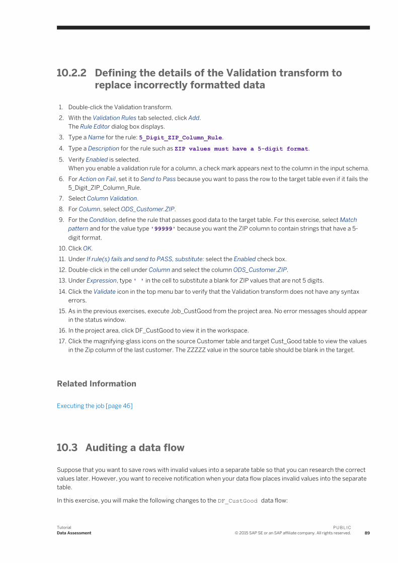
10.2.2 Defining the details of the Validation transform to replace incorrectly formatted data
1. Double-click the Validation transform.2. With the Validation Rules tab selected, click Add.
The Rule Editor dialog box displays.3. Type a Name for the rule: 5_Digit_ZIP_Column_Rule.
4. Type a Description for the rule such as ZIP values must have a 5-digit format.
5. Verify Enabled is selected.When you enable a validation rule for a column, a check mark appears next to the column in the input schema.
6. For Action on Fail, set it to Send to Pass because you want to pass the row to the target table even if it fails the 5_Digit_ZIP_Column_Rule.
7. Select Column Validation.8. For Column, select ODS_Customer.ZIP.9. For the Condition, define the rule that passes good data to the target table. For this exercise, select Match
pattern and for the value type '99999' because you want the ZIP column to contain strings that have a 5-digit format.
10. Click OK.11. Under If rule(s) fails and send to PASS, substitute: select the Enabled check box.12. Double-click in the cell under Column and select the column ODS_Customer.ZIP.13. Under Expression, type ' ' in the cell to substitute a blank for ZIP values that are not 5 digits.
14. Click the Validate icon in the top menu bar to verify that the Validation transform does not have any syntax errors.
15. As in the previous exercises, execute Job_CustGood from the project area. No error messages should appear in the status window.
16. In the project area, click DF_CustGood to view it in the workspace.17. Click the magnifying-glass icons on the source Customer table and target Cust_Good table to view the values
in the Zip column of the last customer. The ZZZZZ value in the source table should be blank in the target.
Related Information
Executing the job [page 46]
10.3 Auditing a data flow
Suppose that you want to save rows with invalid values into a separate table so that you can research the correct values later. However, you want to receive notification when your data flow places invalid values into the separate table.
In this exercise, you will make the following changes to the DF_CustGood data flow:
TutorialData Assessment
P U B L I C© 2015 SAP SE or an SAP affiliate company. All rights reserved. 89
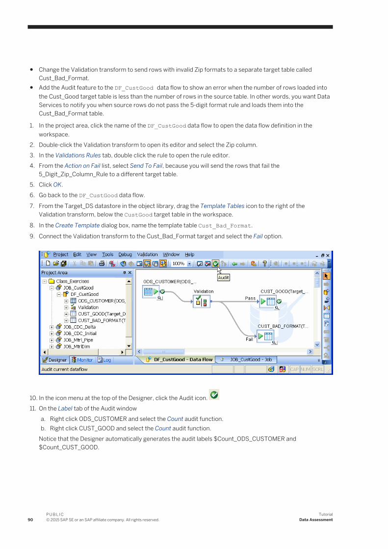
● Change the Validation transform to send rows with invalid Zip formats to a separate target table called Cust_Bad_Format.
● Add the Audit feature to the DF_CustGood data flow to show an error when the number of rows loaded into the Cust_Good target table is less than the number of rows in the source table. In other words, you want Data Services to notify you when source rows do not pass the 5-digit format rule and loads them into the Cust_Bad_Format table.
1. In the project area, click the name of the DF_CustGood data flow to open the data flow definition in the workspace.
2. Double-click the Validation transform to open its editor and select the Zip column.3. In the Validations Rules tab, double click the rule to open the rule editor.4. From the Action on Fail list, select Send To Fail, because you will send the rows that fail the
5_Digit_Zip_Column_Rule to a different target table.5. Click OK.6. Go back to the DF_CustGood data flow.
7. From the Target_DS datastore in the object library, drag the Template Tables icon to the right of the Validation transform, below the CustGood target table in the workspace.
8. In the Create Template dialog box, name the template table Cust_Bad_Format.
9. Connect the Validation transform to the Cust_Bad_Format target and select the Fail option.
10. In the icon menu at the top of the Designer, click the Audit icon. 11. On the Label tab of the Audit window
a. Right click ODS_CUSTOMER and select the Count audit function.b. Right click CUST_GOOD and select the Count audit function.
Notice that the Designer automatically generates the audit labels $Count_ODS_CUSTOMER and $Count_CUST_GOOD.
90P U B L I C© 2015 SAP SE or an SAP affiliate company. All rights reserved.
TutorialData Assessment

12. Click the Rule tab of the Audit window.13. Click Add to enable the expression editor, which consists of three text boxes with drop-down lists:
a. Select the $Count_ODS_CUSTOMER audit label in the first drop-down list.b. Choose the equal sign (=) from the second drop-down list.c. Select the $Count_CUST_GOOD audit label in the third drop-down list.
14. In the Action on failure area on the Rule tab, clear the Raise exception check box because you want the job to continue loading even if rows fail the audit rule.
TutorialData Assessment
P U B L I C© 2015 SAP SE or an SAP affiliate company. All rights reserved. 91
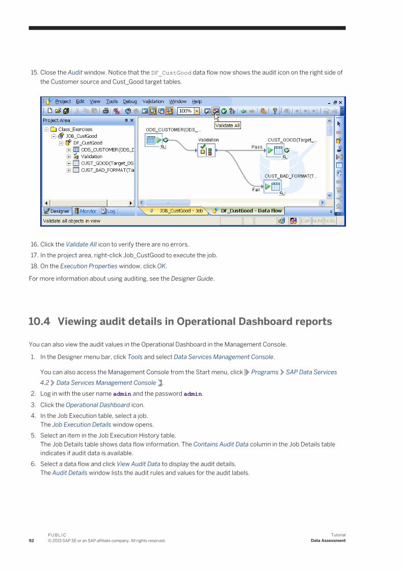
15. Close the Audit window. Notice that the DF_CustGood data flow now shows the audit icon on the right side of the Customer source and Cust_Good target tables.
16. Click the Validate All icon to verify there are no errors.17. In the project area, right-click Job_CustGood to execute the job.18. On the Execution Properties window, click OK.
For more information about using auditing, see the Designer Guide.
10.4 Viewing audit details in Operational Dashboard reports
You can also view the audit values in the Operational Dashboard in the Management Console.
1. In the Designer menu bar, click Tools and select Data Services Management Console.
You can also access the Management Console from the Start menu, click Programs SAP Data Services 4.2 Data Services Management Console .
2. Log in with the user name admin and the password admin.
3. Click the Operational Dashboard icon.4. In the Job Execution table, select a job.
The Job Execution Details window opens.5. Select an item in the Job Execution History table.
The Job Details table shows data flow information. The Contains Audit Data column in the Job Details table indicates if audit data is available.
6. Select a data flow and click View Audit Data to display the audit details.The Audit Details window lists the audit rules and values for the audit labels.
92P U B L I C© 2015 SAP SE or an SAP affiliate company. All rights reserved.
TutorialData Assessment

10.5 Summary and what to do next
In this section you:
● Learned one way to obtain profile statistics● Learned one way to use the validation transform to improve data quality● Defined an audit rule on a data flow to ensure data quality● Viewed audit details
You can now go on to the next section, which describes how to recover from exceptions.
For more information about data assessment, see the Designer Guide.
TutorialData Assessment
P U B L I C© 2015 SAP SE or an SAP affiliate company. All rights reserved. 93

11 Recovery Mechanisms
This section introduces the concepts of recoverable jobs and work flows.
11.1 Creating a recoverable work flow manually
A recoverable work flow is one that can run repeatedly after failure without loading duplicate data. Examples of failure include source or target server crashes or target database errors that could cause a job or work flow to terminate prematurely.
In the following exercise, you will learn how to:
● Design and implement recoverable work flows● Use Data Services conditionals● Specify and use the auto-correction table loader option● Replicate and rename objects in the object library
This exercise creates a recoverable job that loads the sales organization dimension table that was loaded in the section Populating the SalesOrg Dimension from a Flat File [page 38]. You will reuse some of the work completed earlier, which you can revisit at this time if necessary before proceeding.
11.2 Adding the job and defining local variables
1. In the Class_Exercises project, add a new job named JOB_Recovery.2. Open the job and declare these local variables:
Table 24:
Variable Type
$recovery_needed int
$end_time varchar(20)
The $recovery_needed variable determines whether or not to run a data flow in recovery mode. The $end_time variable determines the value of $recovery_needed. These local variables initialize in the script named GetWFStatus (which you will add in the next procedure).
94P U B L I C© 2015 SAP SE or an SAP affiliate company. All rights reserved.
TutorialRecovery Mechanisms

11.3 Specifying a recoverable job
This recoverable job will consist of three objects:
● A script to determine if recovery is required● A conditional to invoke the appropriate data flow● A script to update a status table, signifying successful execution
These objects and their contents are defined in the following sections.
11.3.1 Creating the script that determines the status
First you need to create a script called GetWFStatus.
The script reads the ending time in the status table that corresponds to the most recent start time. The idea is that if there is no ending time for the most recent starting time, the prior data flow invocation must not have completed properly.
1. In JOB_Recovery, add a script to the left side of the workspace and name it GetWFStatus.2. Enter the script contents, which depend on the RDBMS on which status_table resides, as shown in the
following table. Be sure that the SQL statements are on a single line (as opposed to multiple lines, as shown).
NoteThe quotes in the expression $end_time = '' are two single quotes (to denote an empty string).
TutorialRecovery Mechanisms
P U B L I C© 2015 SAP SE or an SAP affiliate company. All rights reserved. 95

Table 25:
RDBMS Script
Oracle $end_time = sql('Target_DS', 'select to_char(end_time, \'YYYY-MM-DD HH24:MI:SS\') from status_table where start_time = (select max(start_time) from status_table)');
if (($end_time IS NULL) or ($end_time = '')) $recovery_needed = 1;
else $recovery_needed = 0;
Microsoft SQL Server,
Sybase ASE
$end_time = sql('Target_DS', 'select convert(char(20), end_time, 0) from status_table where start_time = (select max(start_time) from status_table)');
if (($end_time IS NULL) or ($end_time = '')) $recovery_needed = 1;
else $recovery_needed = 0;
3. Validate the script.
11.3.2 Defining the recoverable data flow with a conditional
You can use a conditional to specify a recoverable data flow. Conditionals have three components:
● A conditional expression to determine an execution path● A work flow to execute for the true branch● A work flow to execute for the false branch
A conditional is a single-use object in work flows that allows you to branch execution logic based on the results of an expression. A conditional takes the form of an if/then/else expression.
11.3.2.1 Adding the conditional
1. Open JOB_Recovery.
2. Click the conditional icon on the tool palette. 3. Click in the workspace to the right of the script GetWFStatus and name the conditional recovery_needed.4. Open the conditional by clicking its name.
The conditional window contains three areas:
○ The if expression○ A box for specifying the work flow to execute if the if condition evaluates true○ A box for specifying the work flow to execute if the if condition evaluates false
96P U B L I C© 2015 SAP SE or an SAP affiliate company. All rights reserved.
TutorialRecovery Mechanisms
5. Specify the if expression. Enter an expression that evaluates to true or false. In this instance, enter:
($recovery_needed = 1)
11.3.2.2 Defining the normal mode work flow
You will reuse the data flow created previously.
1. In the object library, click the Data Flows tab.2. In the Data Flows list, drag DF_SalesOrg into the lower (Else) box of the conditional. This data flow is for the
"false" branch of the conditional.
11.3.2.3 Specifying the recovery mode work flow
The recovery mode work flow will call a modified version of DF_SalesOrg. The only difference is that the Update control for the salesorg_dim target table will have the Auto correct load option enabled. The Auto correct load option causes the table loader to check for existing rows with the same key as each INSERT/UPDATE. When there is a match, the preexisting row will be deleted before inserting a new row (UPDATEs are mapped to INSERTs).
To minimize work in defining this new data flow, the following procedure replicates, renames, and edits DF_SalesOrg for the recovery branch.
1. In the object library, click the Data Flows tab.2. In the Data Flows list, right-click DF_SalesOrg and click Replicate. The replicated data flow will be named
Copy_1_DF_SalesOrg.3. Click the highlighted name and rename the data flow to ACDF_SalesOrg.4. Drag ACDF_SalesOrg to the upper (Then) box of the conditional. This data flow is for the "true" branch of the
conditional.
11.3.2.4 Specifying auto correction for the target table
1. Open the data flow ACDF_SalesOrg.2. Open the target table SALESORG_DIM.3. Click the Options tab. In the Update control area, select the Auto correct load to Yes.
11.3.3 Adding the script that updates the status
This script executes after the work flows in the conditional have completed. Its purpose is to update the status table with the current timestamp to indicate successful execution.
TutorialRecovery Mechanisms
P U B L I C© 2015 SAP SE or an SAP affiliate company. All rights reserved. 97
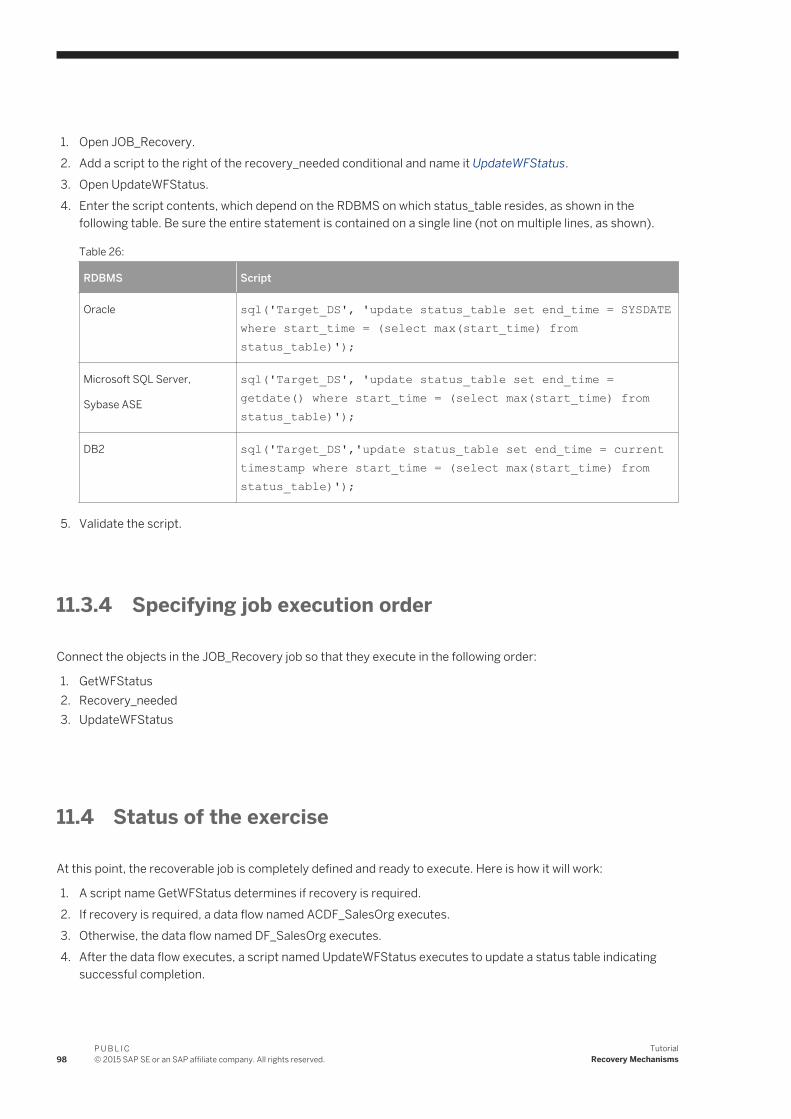
1. Open JOB_Recovery.2. Add a script to the right of the recovery_needed conditional and name it UpdateWFStatus.3. Open UpdateWFStatus.4. Enter the script contents, which depend on the RDBMS on which status_table resides, as shown in the
following table. Be sure the entire statement is contained on a single line (not on multiple lines, as shown).
Table 26:
RDBMS Script
Oracle sql('Target_DS', 'update status_table set end_time = SYSDATE where start_time = (select max(start_time) from status_table)');
Microsoft SQL Server,
Sybase ASE
sql('Target_DS', 'update status_table set end_time = getdate() where start_time = (select max(start_time) from status_table)');
DB2 sql('Target_DS','update status_table set end_time = current timestamp where start_time = (select max(start_time) from status_table)');
5. Validate the script.
11.3.4 Specifying job execution order
Connect the objects in the JOB_Recovery job so that they execute in the following order:
1. GetWFStatus2. Recovery_needed3. UpdateWFStatus
11.4 Status of the exercise
At this point, the recoverable job is completely defined and ready to execute. Here is how it will work:
1. A script name GetWFStatus determines if recovery is required.2. If recovery is required, a data flow named ACDF_SalesOrg executes.3. Otherwise, the data flow named DF_SalesOrg executes.4. After the data flow executes, a script named UpdateWFStatus executes to update a status table indicating
successful completion.
98P U B L I C© 2015 SAP SE or an SAP affiliate company. All rights reserved.
TutorialRecovery Mechanisms
11.5 Executing the job
1. Use a query tool and delete the existing data from the target table SALESORG_DIM.2. Check the contents of status_table and notice that the end_time field is NULL.3. Execute JOB_Recovery.
Because the end_time field is NULL in status_table, the initial execution of this job invokes the recovery-mode data flow.
4. Check the Monitor log to see which data flow was invoked.5. Use a query tool to check the contents of the SALESORG_DIM table. You should see three rows.6. Check the contents of status_table and notice that the end_time field now contains a value.7. Execute the job again.
This time, the non-recovery-mode data flow runs. Verify by examining the monitor log messages.
11.6 Data Services automated recovery properties
Data Services provides job and work flow properties that you can use for automated recovery:
● In the job execution properties, you can select Enable recovery. Then, if the job fails, you will be able to select the job property Recover from last failed execution to skip any steps that successfully completed.
● In work flow properties, you can select Recover as a unit to guarantee that the entire work flow runs again if any part of it requires recovery (per the previous bullet).
11.7 Summary and what to do next
You should now be able to:
● Design and implement recoverable work flows.● Use Data Services conditionals.● Specify and use the Auto correct load option.● Replicate and rename objects in the object library.
The next two sections are optional:
To set up Data Services for multiple users, proceed to the next section.
To use SAP application sources, see Extracting SAP Application Data [page 117].
TutorialRecovery Mechanisms
P U B L I C© 2015 SAP SE or an SAP affiliate company. All rights reserved. 99
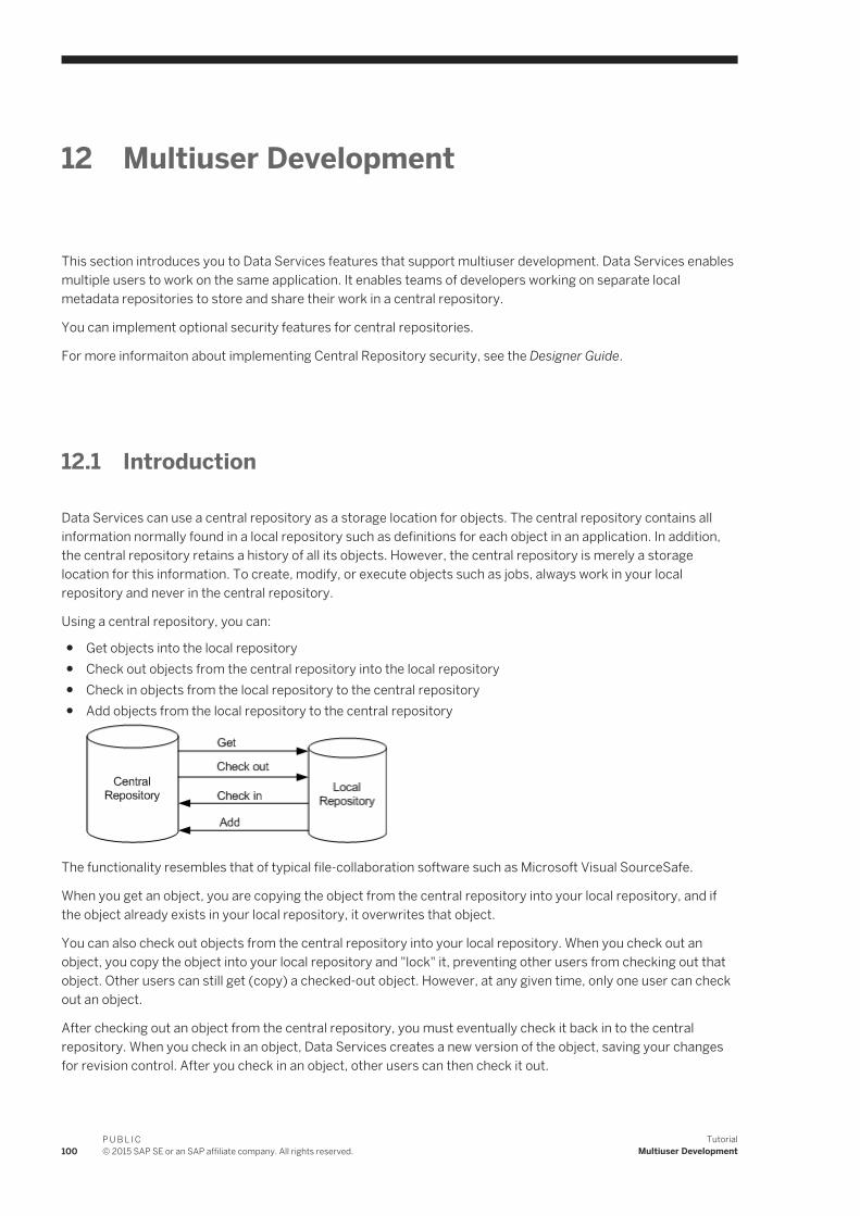
12 Multiuser Development
This section introduces you to Data Services features that support multiuser development. Data Services enables multiple users to work on the same application. It enables teams of developers working on separate local metadata repositories to store and share their work in a central repository.
You can implement optional security features for central repositories.
For more informaiton about implementing Central Repository security, see the Designer Guide.
12.1 Introduction
Data Services can use a central repository as a storage location for objects. The central repository contains all information normally found in a local repository such as definitions for each object in an application. In addition, the central repository retains a history of all its objects. However, the central repository is merely a storage location for this information. To create, modify, or execute objects such as jobs, always work in your local repository and never in the central repository.
Using a central repository, you can:
● Get objects into the local repository● Check out objects from the central repository into the local repository● Check in objects from the local repository to the central repository● Add objects from the local repository to the central repository
The functionality resembles that of typical file-collaboration software such as Microsoft Visual SourceSafe.
When you get an object, you are copying the object from the central repository into your local repository, and if the object already exists in your local repository, it overwrites that object.
You can also check out objects from the central repository into your local repository. When you check out an object, you copy the object into your local repository and "lock" it, preventing other users from checking out that object. Other users can still get (copy) a checked-out object. However, at any given time, only one user can check out an object.
After checking out an object from the central repository, you must eventually check it back in to the central repository. When you check in an object, Data Services creates a new version of the object, saving your changes for revision control. After you check in an object, other users can then check it out.
100P U B L I C© 2015 SAP SE or an SAP affiliate company. All rights reserved.
TutorialMultiuser Development
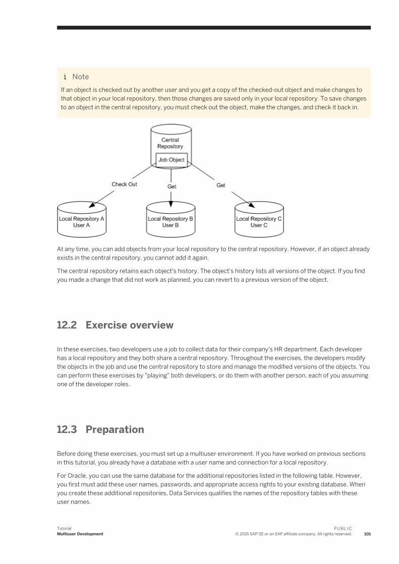
NoteIf an object is checked out by another user and you get a copy of the checked-out object and make changes to that object in your local repository, then those changes are saved only in your local repository. To save changes to an object in the central repository, you must check out the object, make the changes, and check it back in.
At any time, you can add objects from your local repository to the central repository. However, if an object already exists in the central repository, you cannot add it again.
The central repository retains each object's history. The object's history lists all versions of the object. If you find you made a change that did not work as planned, you can revert to a previous version of the object.
12.2 Exercise overview
In these exercises, two developers use a job to collect data for their company's HR department. Each developer has a local repository and they both share a central repository. Throughout the exercises, the developers modify the objects in the job and use the central repository to store and manage the modified versions of the objects. You can perform these exercises by "playing" both developers, or do them with another person, each of you assuming one of the developer roles.
12.3 Preparation
Before doing these exercises, you must set up a multiuser environment. If you have worked on previous sections in this tutorial, you already have a database with a user name and connection for a local repository.
For Oracle, you can use the same database for the additional repositories listed in the following table. However, you first must add these user names, passwords, and appropriate access rights to your existing database. When you create these additional repositories, Data Services qualifies the names of the repository tables with these user names.
TutorialMultiuser Development
P U B L I C© 2015 SAP SE or an SAP affiliate company. All rights reserved. 101
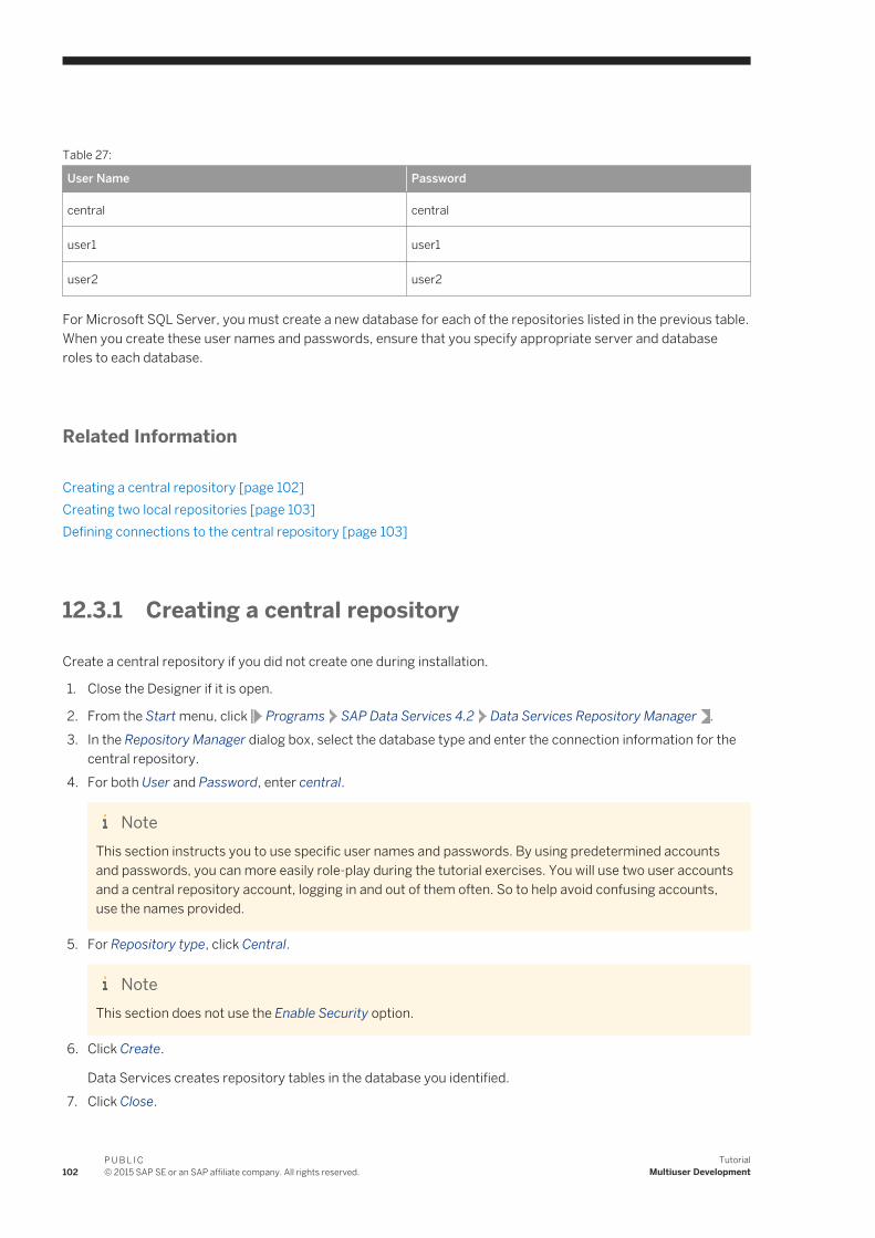
Table 27:
User Name Password
central central
user1 user1
user2 user2
For Microsoft SQL Server, you must create a new database for each of the repositories listed in the previous table. When you create these user names and passwords, ensure that you specify appropriate server and database roles to each database.
Related Information
Creating a central repository [page 102]Creating two local repositories [page 103]Defining connections to the central repository [page 103]
12.3.1 Creating a central repository
Create a central repository if you did not create one during installation.
1. Close the Designer if it is open.
2. From the Start menu, click Programs SAP Data Services 4.2 Data Services Repository Manager .3. In the Repository Manager dialog box, select the database type and enter the connection information for the
central repository.4. For both User and Password, enter central.
NoteThis section instructs you to use specific user names and passwords. By using predetermined accounts and passwords, you can more easily role-play during the tutorial exercises. You will use two user accounts and a central repository account, logging in and out of them often. So to help avoid confusing accounts, use the names provided.
5. For Repository type, click Central.
NoteThis section does not use the Enable Security option.
6. Click Create.
Data Services creates repository tables in the database you identified.7. Click Close.
102P U B L I C© 2015 SAP SE or an SAP affiliate company. All rights reserved.
TutorialMultiuser Development

For more information about implementing Central Repository security, see the Designer Guide.
12.3.2 Creating two local repositories
In a multiuser environment, many users can access a single central repository. Each user must have his or her own local repository in which to work. If you did not create two local repositories during installation, create them using the following procedure.
1. From the Start menu, click Programs SAP Data Services 4.2 Data Services Repository Manager .2. Enter the database connection information for the local repository.3. Type user1 for both User and Password.4. For Repository type, click Local.5. Click Create.6. Type user2 for both User and Password.7. Click Create.8. Click Close.
12.3.3 Associating repositories to your job server
You must associate the local repositories to a job server in order to execute jobs.
1. From the Start menu, click Programs SAP Data Services 4.2 Data Services Server Manager .2. In the SAP Data Services Server Manager dialog box, on the Job Server tab, click Configuration Editor.3. In the Job Server Configuration Editor, select the Job Server Name and click Edit.4. In the Job Server Properties dialog box, in the Associated Repositories area, click Add.5. In the Database type list in the Repository Information area, select the appropriate database type for your
local repository.6. Complete the appropriate connection information for your database type.7. Type user1 in both the User name and Password fields.
8. Click Apply. You should see <databasename>_user1 in the list of Associated Repositories.
9. Repeat steps 4 through 8 to associate user2 to your job server.
10. Click OK to close the Job Server Properties dialog box.11. Click OK to close the Job Server Configuration Editor.12. Click Close and Restart on the Server Manager dialog box.13. Click OK to confirm that you want to restart the Data Services Service.
12.3.4 Defining connections to the central repository
Each local repository requires connection information to any central repository it must access.
TutorialMultiuser Development
P U B L I C© 2015 SAP SE or an SAP affiliate company. All rights reserved. 103
1. Start the Designer and log on to get a list of local repositories.2. Log onto the user1 repository.3. From the Tools menu, click Central Repositories.
In the Designer list, the Central Repository Connections option should be selected.4. Click Add.5. In the Connect to Central repository dialog box, select Central from the list of available repositories and click
OK.6. Click OK.7. Click Yes at the prompt to overwrite the Job Server option parameters.8. Exit the Designer.9. Start Data Services log onto the user2 repository.10. Repeat steps 2 through 8 to establish a connection between the user2 local object library and the central
repository.
12.4 Working in a multiuser environment
After setting up the multiuser environment, you can begin working in it. Remember, Data Services adds all objects to your local repositories.
The tasks in this section include:
● Importing objects into your local repository [page 104]● Activating a connection to the central repository [page 105]● Adding objects to the central repository [page 106]● Checking out objects from the central repository [page 107]● Checking in objects to the central repository [page 108]● Undoing check out [page 109]● Comparing objects [page 110]● Checking out without replacement [page 112]● Getting objects [page 113]● Using filtering [page 114]● Deleting objects [page 115]
12.4.1 Importing objects into your local repository
For these exercises, you will use a job containing previously created work flows and data flows. To use this job, complete the next procedure.
1. Start Data Services and log in as user1 with password user1.Notice that the type of repository, connection, and user ID display above the object library. Use this information to confirm that you logged in to the correct repository.
104P U B L I C© 2015 SAP SE or an SAP affiliate company. All rights reserved.
TutorialMultiuser Development
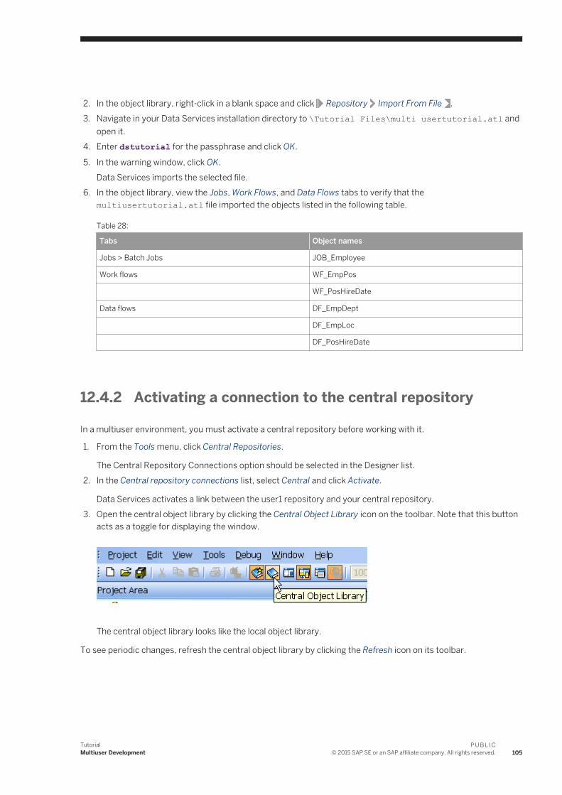
2. In the object library, right-click in a blank space and click Repository Import From File .3. Navigate in your Data Services installation directory to \Tutorial Files\multi usertutorial.atl and
open it.4. Enter dstutorial for the passphrase and click OK.
5. In the warning window, click OK.Data Services imports the selected file.
6. In the object library, view the Jobs, Work Flows, and Data Flows tabs to verify that the multiusertutorial.atl file imported the objects listed in the following table.
Table 28:
Tabs Object names
Jobs > Batch Jobs JOB_Employee
Work flows WF_EmpPos
WF_PosHireDate
Data flows DF_EmpDept
DF_EmpLoc
DF_PosHireDate
12.4.2 Activating a connection to the central repository
In a multiuser environment, you must activate a central repository before working with it.
1. From the Tools menu, click Central Repositories.
The Central Repository Connections option should be selected in the Designer list.2. In the Central repository connections list, select Central and click Activate.
Data Services activates a link between the user1 repository and your central repository.3. Open the central object library by clicking the Central Object Library icon on the toolbar. Note that this button
acts as a toggle for displaying the window.
The central object library looks like the local object library.
To see periodic changes, refresh the central object library by clicking the Refresh icon on its toolbar.
TutorialMultiuser Development
P U B L I C© 2015 SAP SE or an SAP affiliate company. All rights reserved. 105

12.4.3 Adding objects to the central repository
After importing objects into the user1 local repository, you can add them to the central repository for storage. When adding objects to the central repository, you can add a single object or the object and its dependents. All projects and objects in the object library can be stored in a central repository.
Related Information
Objects and their hierarchical relationships [page 38]
12.4.3.1 Adding a single object to the central repository
1. Click the Formats tab in the user1 local object library.2. Expand Flat Files to display the file names.
3. Right-click NameDate_Format and click Add to Central Repository Object .
Data Services prompts you to add optional comments about adding this object to the central repository.4. Click OK.
Data Services adds the object to the active central repository. The Output window opens to indicate that Data Services added the object successfully.
NoteThe Add to Central Repository command will not be available if the object already exists in the central repository.
5. If it is not already open, open the central object library by clicking its icon on the toolbar.
NoteYou can add the central object library to the Designer window by dragging it over the window and one of the arrows that each represent a location where you can place the library. Each arrow displays the shape and location of where the library will fit. To separate again, drag the central object library away from the Designer window.
6. Click the Formats tab of the Central object library and verify that NameDate_Format is listed under Flat Files.
12.4.3.2 Adding an object and its dependents to the central repository
1. Click the Work Flows tab in the user1 local object library.
106P U B L I C© 2015 SAP SE or an SAP affiliate company. All rights reserved.
TutorialMultiuser Development

2. Double-click WF_EmpPos and notice that DF_EmpDept and DF_EmpLoc are inside it.
3. Right-click WF_EmpPos and click Add to Central Repository Object and dependents . The Comments window opens.
4. In the comments field, type:
Adding WF_EmpPos, DF_EmpDept, and DF_EmpLoc to the central repository. 5. Click Apply to all.6. Close the Output window. (The toolbar also has a toggle button for the Output window.)7. In the central object library, click the Data Flows tab and verify that the DF_EmpDept and DF_EmpLoc data
flows are listed under Data Flows.8. Click the Work Flows tab of the central object library.9. In the Work Flows tab of the local object library, drag the WF_PosHireDate work flow to the work flow tab of
the central object library, which will add it and its data flow (DF_PosHireDate) to the central repository.10. In the Version Control Confirmation window, click Next.11. In the Datastore Options window, click Finish.
NoteIf you see an alert that some objects already exist in the repository, click Yes to continue.
12. In the Comments dialog box, type:
Adding WF_PosHireDate and DF_PosHireDate to the central repository 13. Click Apply to all.14. Click the Data Flows tab in the central object library and verify that the DF_PosHireDate data flow is listed
under Data Flows.
Now that the central repository contains all objects in the user1 local repository, developers can check out, check in, label, and get those objects.
12.4.4 Checking out objects from the central repository
When you check out an object, it becomes unavailable to other users. Other users can view the object but cannot make changes to it. You can check out a single object or check out an object with all of its dependents.
If you check out a single object such as WF_EmpPos, then you cannot change its dependents (such as DF_EmpDept) and save those changes in the central repository. You can only save changes to dependent objects that are not checked out in your local repository.
Alternatively, if you check out WF_EmpPos with all of its dependents, you can make changes to the dependent objects (DF_EmpDept or DF_EmpLoc). Because you checked out the dependents, you can save changes in both the central repository and your local repository.
TutorialMultiuser Development
P U B L I C© 2015 SAP SE or an SAP affiliate company. All rights reserved. 107

12.4.4.1 Checking out an object and its dependent objects
1. Open the central object library.2. In the central object library, right-click the WF_EmpPos work flow.
3. Click Check Out Object and dependents .
Alternatively, you can select the object in the central object library, then click the Check out object and dependents icon on the central object library toolbar.
Data Services copies the most recent version of WF_EmpPos and its dependent objects from the central repository into the user1 local repository. A red check mark appears on the icon for objects that are checked out in both the local and central repositories.
While user1 has the WF_EmpPos work flow checked out, he or she can modify it or its dependents in the user1 local repository.
12.4.4.2 Modifying dependent objects in the WF_EmpPos work flow
1. In the local object library, click the Data Flows tab.2. Open the DF_EmpDept data flow.3. In the DF_EmpDept workspace, double-click the query icon's name to open the query editor.4. Change the mapping: Right-click FName in the target schema (Schema Out) and click Cut.5. Click the Back arrow in the icon bar to return to the data flow.6. Open the DF_EmpLoc data flow.7. Click the query icon's name to open the query editor.8. Change the mapping:
a. Right-click FName in the target schema and click Cut.b. Right-click LName in the target schema and click Cut.
9. From the Project menu, click Save All (even though there are no actual projects open).10. Click OK to save your changes.
Next, user1 will check in one of the modified objects.
12.4.5 Checking in objects to the central repository
You can check in an object by itself or check it in along with all associated dependent objects. When an object and its dependents are checked out and you check in the single object without its dependents, the dependent objects remain checked out.
108P U B L I C© 2015 SAP SE or an SAP affiliate company. All rights reserved.
TutorialMultiuser Development
12.4.5.1 Checking in a single object
1. Open the central object library.
2. Right-click the DF_EmpDept data flow in the central object library and click Check In Object .
A Comment window opens.3. In the comments field, type:
Removed FName and LName columns from NAMEDEPT target table 4. Click OK.
Data Services copies the object from the user1 local repository to the central repository and removes the check-out marks.
5. In the central object library window, right-click DF_EmpDept and click Show History.6. Close the History window and Exit Data Services.
The next portion of this exercise involves a second developer (user2).
12.4.5.2 Setting up the second developer's environment
1. Start the Designer and log into the user2 repository.2. Import the multiusertutorial.atl file.
Enter dstutorial for the passphrase, and click OK.
3. Activate the connection to the central repository.4. Open the central object library.5. Notice that you cannot check out DF_EmpLoc because it is still checked out by user1.
Related Information
Activating a connection to the central repository [page 105]Importing objects into your local repository [page 104]
12.4.6 Undoing check out
Suppose you check out DF_PosHireDate from the central repository and begin modifying it in your local repository. Then you realize you are working with the wrong data flow—you intended to modify DF_EmpLoc. In this situation, you can undo the check out of DF_PosHireDate from the central repository.
When you undo a check out, you leave the object in the central repository as is. Data Services does not save changes or create a new version in the central repository. Your local repository, however, retains any changes you made. To undo changes in the local repository, you must get a copy of the current, unchanged object from the central repository.
TutorialMultiuser Development
P U B L I C© 2015 SAP SE or an SAP affiliate company. All rights reserved. 109

Undo check out works for both a single object as well as objects with dependents.
In the next exercise, user2 will check out objects from the central repository, modify the objects in the user2 local object library, and then undo the check out.
Related Information
Getting objects [page 113]
12.4.6.1 Checking out and modifying the DF_PosHireDate data flow
1. Open the central object library.
2. In the central object library, right-click the DF_PosHireDate data flow and click Check Out Object .3. In the local object library, open the DF_PosHireDate data flow.4. Click the query icon's name.5. Change the mapping: Right-click LName in the target schema and click Cut.6. From the Project menu, click Save All.7. Click OK.
Now suppose you realize you modified the wrong data flow. You intended to modify the DF_EmpLoc data flow instead.
12.4.6.2 Undoing a check out of the DF_PosHireDate data flow
In the central object library, right-click DF_PosHireDate and click Undo Check Out Object .
Data Services removes the check-out symbol from DF_PosHireDate without saving changes to it in the central repository. In the next procedure, you will verify this by comparing the copy of DF_PosHireDate in the user2 local object library to the version of DF_PosHireDate in the central repository.
12.4.7 Comparing objects
Data Services allows you to compare two objects from local and central repositories to determine the differences, if any, between those objects.
In this exercise, the second developer will compare the copy of the DF_PosHireDate data flow in the user2 local object library to the version of the DF_PosHireDate data flow in the central repository to verify the undo check-out performed in Undoing check out [page 109].
110P U B L I C© 2015 SAP SE or an SAP affiliate company. All rights reserved.
TutorialMultiuser Development

1. From the user2 local object library, right-click DF_PosHireDate and click Compare Object with dependents to Central .
The Difference Viewer opens in the workspace.
2. The query icon in the left pane shows the consolidated symbol, so click the plus symbol to expand the object
tree and find the changed object.
The Differences Viewer indicates that the LName column is missing in the local copy, but the central repository copy still shows the previous version of DF_PosHireDate with the LName column present.
Data Services shows the differences between the two objects in the panes. If there are no differences, the status bar below the panes indicates Difference [ ] of 0. If there are differences between the objects, Data Services indicates each difference with a symbol and highlights the affected objects. The left side of the status bar shows the key to the symbols and the meaning of each, as described in the following table.
Table 29:
Icon Difference Description
Deleted The item does not appear in the object in the right pane.
Changed The differences between the items are highlighted in blue (the default) text.
Inserted The item has been added to the object in the right pane.
Consolidated This icon appears next to an item if items within it have differences. Expand the item by clicking its plus sign to view the differences
TutorialMultiuser Development
P U B L I C© 2015 SAP SE or an SAP affiliate company. All rights reserved. 111

12.4.8 Checking out without replacement
Suppose you continue to work in the user2 local object library and modify the DF_EmpLoc data flow. After modifying it, you want to place your copy of this data flow in the central repository. However, you never checked out DF_EmpLoc from the central repository. If you now checked out DF_EmpLoc from the central repository, Data Services would copy the most recent version from the central repository into the user2 local object library, overwriting your local copy. All your work on your copy of DF_EmpLoc would be lost.
Data Services provides an option that allows you to check out an object without copying the latest version of the object from the central repository into your local repository. This option is called checking out without replacement. You can check out a single object or an object and its dependents without replacement.
In the next exercise, the second developer will modify the DF_EmpLoc data flow in the user2 local object library, check it out without replacement, and then check his unaltered, local copy of the data flow back in to the central repository.
12.4.8.1 Modifying the data flow DF_EmpLoc
1. In the local repository, open the DF_EmpLoc data flow.2. Click the query icon's name to open the query editor.3. Change the mapping: Right-click FName in the output schema and click Cut.4. From the Project menu, click Save All to save your work.
Now you realize that you want to place your copy of DF_EmpLoc in the central repository.
12.4.8.2 Checking out an object without replacement
1. Open the central object library.
2. In the central object library, right-click DF_EmpLoc and click Check Out Object without replacement .
Now the DF_EmpLoc data flow in the central repository is "locked" so other users cannot check it out, but the copy of the DF_EmpLoc data flow in the user2 local object library remains unchanged.
12.4.8.3 Checking in the DF_EmpLoc data flow
1. From the central repository, check in the DF_EmpLoc data flow. In the Comment field of the Check In window, type Removed FName from POSLOC, and click OK.
(See Checking in objects to the central repository [page 108].)
Now the central repository contains a third version of DF_EmpLoc. This version is the same as the copy of DF_EmpLoc in the user2 local object library.
2. Compare the copy of DF_EmpLoc in the user2 local object library with the third version of DF_EmpLoc in the central repository to verify they are the same.
112P U B L I C© 2015 SAP SE or an SAP affiliate company. All rights reserved.
TutorialMultiuser Development

(See Comparing objects [page 110].)3. Exit Data Services.
Next, the first developer (user1) will check in the DF_EmpDept data flow into the central repository. Then no objects will be checked out of the central repository.
12.4.8.4 Checking in DF_EmpDept and WF_EmpPos
1. Start the Designer and log back in as user1 with password user1.2. Open the central object library.
NoteRemember to reactivate the connection to the central repository from user1 (see Activating a connection to the central repository [page 105]).
3. Check in DF_EmpDept, and type Removed FName from NAMEDEPT in the Comment field. (See Checking in objects to the central repository [page 108].)
4. Click Yes in the Check In Warning window.
Now the central repository contains three versions of DF_EmpLoc, two versions of DF_EmpDept, and one version of DF_PosHireDate.
5. To confirm, right-click each object and click Show History.6. Check in WF_EmpPos without dependents and type Modified DF_EmpLoc and DF_EmpDept in the Comment
field.
12.4.9 Getting objects
You might want to copy a specific version of an object from the central repository into your local repository. Getting objects allows you to do so. When you get an object, you copy a version of that object from the central repository into your local repository, replacing the version in your local repository. Getting an object is not equivalent to checking out an object.
12.4.9.1 Getting the latest version of an object
1. In the local object library, open the DF_EmpLoc data flow.2. Click the query icon's name to open the query editor.3. Make note of the Pos and Loc columns in the target schema (POSLOC target table.).4. Click the Back arrow in the icon bar to return to the data flow.
5. In the central object library, right-click the DF_EmpLoc data flow in the central object library and click Get Latest Version Object .
TutorialMultiuser Development
P U B L I C© 2015 SAP SE or an SAP affiliate company. All rights reserved. 113
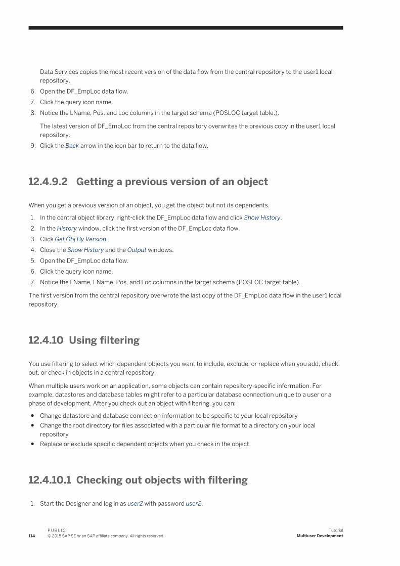
Data Services copies the most recent version of the data flow from the central repository to the user1 local repository.
6. Open the DF_EmpLoc data flow.7. Click the query icon name.8. Notice the LName, Pos, and Loc columns in the target schema (POSLOC target table.).
The latest version of DF_EmpLoc from the central repository overwrites the previous copy in the user1 local repository.
9. Click the Back arrow in the icon bar to return to the data flow.
12.4.9.2 Getting a previous version of an object
When you get a previous version of an object, you get the object but not its dependents.
1. In the central object library, right-click the DF_EmpLoc data flow and click Show History.2. In the History window, click the first version of the DF_EmpLoc data flow.3. Click Get Obj By Version.4. Close the Show History and the Output windows.5. Open the DF_EmpLoc data flow.6. Click the query icon name.7. Notice the FName, LName, Pos, and Loc columns in the target schema (POSLOC target table).
The first version from the central repository overwrote the last copy of the DF_EmpLoc data flow in the user1 local repository.
12.4.10 Using filtering
You use filtering to select which dependent objects you want to include, exclude, or replace when you add, check out, or check in objects in a central repository.
When multiple users work on an application, some objects can contain repository-specific information. For example, datastores and database tables might refer to a particular database connection unique to a user or a phase of development. After you check out an object with filtering, you can:
● Change datastore and database connection information to be specific to your local repository● Change the root directory for files associated with a particular file format to a directory on your local
repository● Replace or exclude specific dependent objects when you check in the object
12.4.10.1 Checking out objects with filtering
1. Start the Designer and log in as user2 with password user2.
114P U B L I C© 2015 SAP SE or an SAP affiliate company. All rights reserved.
TutorialMultiuser Development

2. Open the central object library.
3. Right-click WF_EmpPos and click Check Out With filtering .
The Version Control Confirmation window shows your selected object and any dependent objects.4. Click the plus symbol to expand the Flat Files list.5. Click NamePos_Format, and in the Target status list click exclude.
NamePos_Format will not be checked out.6. Click Next.7. The Datastore Options window shows any datastores used by the object. This window only opens if the
objects that you are adding, checking in, or checking out include a datastore. Click Finish.
12.4.11 Deleting objects
You can delete objects from the local or the central repository.
12.4.11.1 Deleting an object from the central repository
1. Still logged on as user2, open the central object library.2. On the Work Flows tab, right-click WF_PosHireDate and click Delete. Click OK to confirm deletion.
When you delete objects from the central repository, you delete only the selected object and all versions of it; you do not delete any dependent objects.
3. In the central object library, click the Data Flows tab and verify that DF_PosHireDate was not deleted from the central repository.
When you delete an object from a central repository, it is not automatically deleted from the connected local repositories.
4. Open the Work Flows tab in the local object library to verify that WF_PosHireDate was not deleted from the user2 local object library.
12.4.11.2 Deleting an object from a local repository
1. Click the Data Flows tab in the user2 local object library.2. Right-click DF_EmpDept and click Delete.
When you delete an object from a local repository, it does not get deleted from the active central repository. In fact, you can get or check out an object from the central repository to reinsert it.
3. Open the central object library.4. Click Refresh on the toolbar.5. In the central repository, click the Data Flows tab and verify that DF_EmpDept was not deleted from the
central repository.
TutorialMultiuser Development
P U B L I C© 2015 SAP SE or an SAP affiliate company. All rights reserved. 115

6. Exit Data Services.
12.5 Summary and what to do next
You have created two local repositories and one central repository and performed the tasks associated with sharing objects using Data Services.
For more information about the topics covered in this section, see the Data Services Designer Guide.
116P U B L I C© 2015 SAP SE or an SAP affiliate company. All rights reserved.
TutorialMultiuser Development

13 Extracting SAP Application Data
This optional section introduces the SAP Data Services objects for extracting data from SAP application sources:
● SAP Applications datastores● ABAP data flows● transports
NoteThe procedures in this section require that the software has the ability to connect to an SAP server. The sample tables provided with Data Services that are used in these procedures do not work with all versions of SAP because the structure of standard SAP tables varies in different versions.
13.1 Defining an SAP Applications datastore
1. In the local object library, click the Datastores tab.2. Right-click inside the blank space and click New.
The Datastore Editor dialog box opens.3. In the Datastore name field, type SAP_DS.
This name identifies the database connection inside the software.
TutorialExtracting SAP Application Data
P U B L I C© 2015 SAP SE or an SAP affiliate company. All rights reserved. 117

4. In the Datastore type list, click SAP Applications to specify the datastore connection path to the database.5. In the Application server field, type the name of the remote SAP Applications computer (host) to which Data
Services connects.6. Enter the user name and password for the SAP applications Server.7. Click OK.
Data Services saves your SAP application database connection to the metadata repository.
13.2 Importing metadata for individual SAP application source tables
You will now import metadata from SAP application tables into Data Services.
1. In the object library on the Datastores tab, right-click SAP_DS and click Import by Name.2. In the Type list, click Table.3. In the Name box, type KNA1.4. Click OK.5. Repeat steps 1 through 4 for the other SAP tables you will need:
○ MAKT○ MARA○ VBAK○ VBAP○ VBUP
6. In the object library, expand SAP_DS, then expand Tables to display the imported SAP tables:
118P U B L I C© 2015 SAP SE or an SAP affiliate company. All rights reserved.
TutorialExtracting SAP Application Data
13.3 Repopulating the customer dimension table
You will now repopulate the customer dimension table from SAP. First you will define a data flow that calls an ABAP data flow to extract SAP data and load it into the customer dimension table.
13.3.1 Adding the SAP_CustDim job, work flow, and data flow
13.3.1.1 Adding the job
1. Open the Class_Exercises project.2. Right-click the project name and click New Batch Job.3. Rename the job JOB_SAP_CustDim.
13.3.1.2 Adding the work flow
1. Open JOB_SAP_CustDim by clicking on its name in the project area.2. Add a new work flow and name it WF_SAP_CustDim.
13.3.1.3 Adding the data flow
1. Click the WF_SAP_CustDim work flow name to open it.2. Add a new data flow to the work flow definition and name it DF_SAP_CustDim.
3. Click the name of the data flow to open its definition.
13.3.2 Defining the SAP_CustDim data flow
So far, you have followed similar procedures as in previous sections. Now, however, because you are loading data from an SAP application, the procedure to define the data flow is somewhat different.
The data flow for building the dimension table will consist of the following objects:
● A data flow to read data from an SAP table and perform any other operations that need to happen in SAP.● The target table into which the customer dimension data loads.
TutorialExtracting SAP Application Data
P U B L I C© 2015 SAP SE or an SAP affiliate company. All rights reserved. 119

13.3.2.1 Naming the source and target tables
1. Ensure the DF_SAP_CustDim data flow is open in the workspace.
2. Click the ABAP data flow icon on the tool palette. 3. Click in the workspace to place the ABAP data flow.
A window appears prompting you for the SAP applications properties.4. On the Options tab, complete the following fields:
a. Datastore: Click SAP_DS.b. Generated ABAP file name: Specify the name of the file that will contain the ABAP code generated by the
software. This file will be created in the Generated ABAP directory specified in the SAP_DS datastore.c. ABAP program name: This is the ABAP program name that will be uploaded into SAP applications. It must
begin with the letter Y or Z and not exceed eight characters.d. Job name: Type SAP_CustDim. This is the job name that will run in SAP applications.
5. Click OK.
A representation of the ABAP data flow appears in the workspace and the project area.6. Name the data flow DF_ABAP_CustDim.7. In the object library, click the Datastores tab and for the Target_DS datastore, expand the Tables list.
120P U B L I C© 2015 SAP SE or an SAP affiliate company. All rights reserved.
TutorialExtracting SAP Application Data

8. Drag the CUST_DIM table into the workspace, drop it to the right of the ABAP data flow DF_ABAP_CustDim, and click Make Target from the shortcut menu.
13.3.3 Defining the ABAP data flow
There are two more components that you must add before all of the objects necessary to populate the customer dimension table are present.
At this point you must:
● Designate the source table named KNA1● Define the query that specifies what data to extract● Define the data transport object into which SAP applications writes the resulting data set● Define the order of execution
13.3.3.1 Bringing the components into the ABAP data flow
1. Click the name of the DF_ABAP_CustDim data flow to open its definition.2. In the object library, click the Datastores tab and for the SAP_DS datastore, expand the Tables list.3. Drag the KNA1 table into the workspace and drop it on the left side.
4. Click the query icon in the tool palette and place it to the right of the table in the workspace.
5. Click the data transport icon in the tool palette and place it to the right of the query in the workspace. 6. Connect the icons to indicate the flow of data as shown.
TutorialExtracting SAP Application Data
P U B L I C© 2015 SAP SE or an SAP affiliate company. All rights reserved. 121

13.3.3.2 Defining the query
1. In the workspace, click the name of the query to open the query editor.2. Expand table KNA1 to see its columns.3. Click the column head (above the table name) to sort the list in alphabetical order.4. Map the following seven source columns to the target schema. Use Ctrl-click to select multiple columns and
drag them to the output schema.○ KUKLA○ KUNNR○ NAME1○ ORT01○ PSTLZ○ REGIO○ STRAS
The Mapping tab of the property sheet shows the mapping relationship, and the icon next to the source column changes to an arrow to indicate that the column has been mapped.
5. Referring to the following table, rename the target columns and verify or change data types and descriptions by right-clicking each name in the output schema and clicking Properties.
Table 30:
Original name New name Data type Description
KUNNR Cust_ID varchar(10) Customer number
KUKLA Cust_classf varchar(2) Customer classification
NAME1 Name1 varchar(35) Customer name
STRAS Address varchar(35) Address
ORT01 City varchar(35) City
REGIO Region_ID varchar(3) Region
PSTLZ Zip varchar(10) Postal code
NoteIn Microsoft SQL Server and Sybase ASE, the columns must be specified in the order shown here, not alphabetically.
122P U B L I C© 2015 SAP SE or an SAP affiliate company. All rights reserved.
TutorialExtracting SAP Application Data
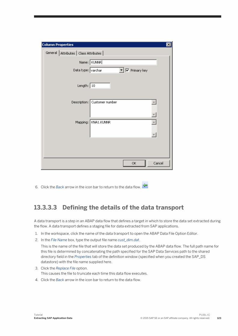
6. Click the Back arrow in the icon bar to return to the data flow.
13.3.3.3 Defining the details of the data transport
A data transport is a step in an ABAP data flow that defines a target in which to store the data set extracted during the flow. A data transport defines a staging file for data extracted from SAP applications.
1. In the workspace, click the name of the data transport to open the ABAP Data File Option Editor.2. In the File Name box, type the output file name cust_dim.dat.
This is the name of the file that will store the data set produced by the ABAP data flow. The full path name for this file is determined by concatenating the path specified for the SAP Data Services path to the shared directory field in the Properties tab of the definition window (specified when you created the SAP_DS datastore) with the file name supplied here.
3. Click the Replace File option.This causes the file to truncate each time this data flow executes.
4. Click the Back arrow in the icon bar to return to the data flow.
TutorialExtracting SAP Application Data
P U B L I C© 2015 SAP SE or an SAP affiliate company. All rights reserved. 123

13.3.3.4 Defining the execution order for the data flow
1. Click the Back arrow again to open the DF_ABAP_CustDim data flow in the workspace.2. Click and drag to connect the output of the DF_ABAP_CustDim data flow to the input of the CUST_DIM table.
13.3.4 Validating the SAP_CustDim data flow
Next you will verify that the data flow has been constructed properly.
Click the Validate All button on the toolbar.
If your design contains errors, a message appears describing the error, which requires solving before you can proceed.
A warning message provides information only and does not interfere with proper job execution.
If your data flow contains no errors, you will see the message:
Validate: No errors found
13.3.5 Executing the SAP_CustDim job
13.3.5.1 Executing the JOB_SAP_CustDim job
1. Right-click the job name in the project area and click Execute.
You will be prompted to save your work.2. Click OK.
The job executes after you save your work. The Execution Properties dialog box appears. Use the default settings.
After the job completes, check the Output window for any error or warning messages (there should be none; see the next section if you get ABAP errors).
3. Using a query tool, check the contents of the cust_dim table.
13.3.6 About ABAP job execution errors
The following table describes some common ABAP job execution errors.
124P U B L I C© 2015 SAP SE or an SAP affiliate company. All rights reserved.
TutorialExtracting SAP Application Data

Table 31:
Error Probable cause Solution
Cannot open ABAP output file
Lack of permissions for Job Server service account.
Open the Services Control Panel, double-click the Data Services service, and select a user account with permissions to the working folder on the SAP server.
Cannot create ABAP output file
Working directory on SAP server specified incorrectly.
In the object library on the Datastores tab, right-click the SAP datastore and click Edit. Review the Working Directory on SAP Server box and edit if necessary. Verify by copying the path
and pasting it into the Start Run dialog box and executing. This should open a window to the working directory on the SAP server.
13.4 Repopulating the material dimension table
You will now repopulate the material dimension table from SAP. This data flow is similar to the customer dimension data flow except that the data for the material dimension table is the result of a join between two SAP application tables.
13.4.1 Adding the SAP_MtrlDim job, work flow, and data flow
13.4.1.1 Adding the job
1. Open the Class_Exercises project.2. Right-click the project name and click New Batch Job.3. Rename the job JOB_SAP_MtrlDim.
13.4.1.2 Adding the work flow
1. Open JOB_SAP_MtrlDim by clicking on its name in the project area.2. Add a new work flow and name it WF_SAP_MtrlDim.
TutorialExtracting SAP Application Data
P U B L I C© 2015 SAP SE or an SAP affiliate company. All rights reserved. 125

13.4.1.3 Adding the data flow
1. Click the WF_SAP_MtrlDim work flow name to open its definition.2. Add a new data flow to the work flow definition and name it DF_SAP_MtrlDim.
3. Click the name of the data flow to open its definition.
13.4.2 Defining the DF_SAP_MtrlDim data flow
The data flow for building a material dimension table will consist of the following objects:
● An ABAP data flow to read data from an SAP table and perform any other operations that need to happen in the SAP database.
● Target table into which the material dimension data loads.
13.4.2.1 Naming the source and target tables
1. Ensure the DF_ABAP_MtrlDim data flow is open in the workspace.
2. Click the ABAP data flow icon in the tool palette. 3. Click in the workspace.
A dialog box appears prompting you for properties.4. On the Options tab, complete the following fields:
a. Datastore: Click SAP_DS.b. Generated ABAP file name: Specify the name of the file that will contain the ABAP code generated by the
software. This file will be created in the Generated ABAP directory specified in the SAP_DS datastore (for example mtrldim.aba).
c. ABAP program name: This is the ABAP program name that will be uploaded into SAP. It must begin with the letter Y or Z and not exceed eight characters (for example zmtrldim.)
d. Job name: Type SAP_MtrlDim. This is the job name that will run in SAP.5. Click the General tab and name the data flow DF_ABAP_MtrlDim.6. Click OK.
A representation of the data flow appears in the workspace and project area.7. In the object library, click the Datastores tab and for the Target_DS datastore, expand the Tables list.8. Drag the MTRL_DIM table into the workspace, drop it to the right of the data flow DF_ABAP_MtrlDim, and click
Make Target from the shortcut menu.
13.4.3 Defining the data flow
Next, designate the two source tables MARA and MAKT, then:
126P U B L I C© 2015 SAP SE or an SAP affiliate company. All rights reserved.
TutorialExtracting SAP Application Data

● Define a query to join these tables and determine from which columns to read data● Define a data transport into which the SAP application writes the resulting data set● Define the order of execution
13.4.3.1 Bringing the components into the data flow
1. Click the name of the DF_ABAP_MtrlDim data flow to open its definition.2. In the object library, click the Datastores tab and for the SAP_DS datastore, expand the Tables list.3. Drag the MARA table into the workspace and drop it on the left side.4. Drag the MAKT table into the workspace and drop it on the left side below the MARA table.
5. Click the query transform icon in the tool palette and place it to the right of the table in the workspace.
6. Click the data transport icon in the tool palette and place it to the right of the query in the workspace. 7. Connect the icons to indicate the flow of data as shown.
TutorialExtracting SAP Application Data
P U B L I C© 2015 SAP SE or an SAP affiliate company. All rights reserved. 127

13.4.3.2 Defining the details of the query including the join between source tables
1. Click the name of the query to open the query editor.2. In the FROM tab, in the Join pairs area, select MARA from the Left drop-down list.3. Select MAKT from the Right drop-down list.
Similar to the where clause of a SQL statement, the FROM tab in this query contains the conditions that the source rows must meet to be passed to the target including the join relationship between sources.
The resulting relationship appears in the From clause text box:
(MARA.MATNR = MAKT.MATNR)
4. Click the smart editor icon. 5. In the Smart Editor, type the following text. Use all uppercase, as shown. This statement filters the material
descriptions by language and brings the only English-language material records into the target.
AND (SPRAS = 'E')
6. Click OK.7. Map the following source columns to output columns. Remember that to map the contents of a column,
select the column in the source schema and drag it to the target schema.
Table 32:
Table Column
MARA MATNR
MTART
MBRSH
MATKL
MAKT MAKTX
8. As described in the following table, rename the target columns, verify data types, and add descriptions.To change the name or description of a target column, double-click the column name (or right-click and click Properties). In the Properties window, type the new column name and description.
Use the following column names, data types, and descriptions:
Table 33:
Original name New name Data type Description
MATNR Mtrl_id varchar(18) Material number
MTART Mtrl_typ varchar(4) Material type
MBRSH Ind_sector varchar(1) Industry sector
MATKL Mtrl_grp varchar(9) Material group
MAKTX Descr varchar(60) Material description
9. Click the Back arrow in the icon bar to return to the data flow.
128P U B L I C© 2015 SAP SE or an SAP affiliate company. All rights reserved.
TutorialExtracting SAP Application Data

13.4.3.3 Defining data transport details
1. Click the name of the data transport object to open the ABAP Data File Option Editor.2. Enter the output file name in the File Name box:
mtrl_dim.datThis is where the data set produced by the data flow will be stored.
3. Click Replace File.This truncates the file each time the data flow runs.
4. Click the Back arrow in the icon bar.
13.4.3.4 Defining the order of execution for the data flow
1. Ensure the DF_ABAP_MtrlDim data flow is open in the workspace.2. Connect the right side of DF_ABAP_MtrlDim to the left side of the mtrl_dim table.3. Click the Validate All button on the toolbar.
If your design contains errors, a dialog box appears with a message describing the error. As before, warning messages are OK.
13.4.4 Executing the SAP_MtrlDim job
1. Execute the job named JOB_SAP_MtrlDim as you did in Executing the SAP_CustDim job [page 124]. Check the Output window for any error or warning messages.
2. Using a query tool, check the MTRL_DIM table.3. From the Project menu, click Save All.
13.5 Repopulating the SalesFact table
The exercise populates a sales fact table from an SAP application source. You will also add a column to one of the output schemas that allows you to access a value in another table using a lookup.
13.5.1 Adding the SAP_SalesFact job, work flow, and data flow
1. Add the job that will load data into the sales fact table and name it JOB_SAP_SalesFact.
2. Open the job definition, add the work flow for the sales fact table and name it WF_SAP_SalesFact.
3. Open the work flow definition, add the data flow for the sales fact table and name it DF_SAP_SalesFact.
TutorialExtracting SAP Application Data
P U B L I C© 2015 SAP SE or an SAP affiliate company. All rights reserved. 129
13.5.2 Defining the DF_SAP_SalesFact data flow
The data flow instructions for building the fact table are the same as the previous section's exercise. The data flow consists of the following objects:
● An ABAP data flow to read data from an SAP application table and perform any other operations that need to happen in the SAP database
● The target file into which the customer dimension data loads
Related Information
Defining the DF_SAP_MtrlDim data flow [page 126]
13.5.2.1 Naming the source and target tables
1. Click the name of the data flow to open the data flow definition.
2. Click the ABAP data flow icon in the tool palette. 3. Click a location in the workspace to place the data flow.
A dialog box appears prompting you for properties.4. Complete the following fields:
a. Datastore: Click SAP_DS.b. Generated ABAP file name: Specify the name of the file that will contain the ABAP code that software
generates. This file will be created in the Generated ABAP directory specified in the SAP_DS datastore (for example SalesFact.aba).
c. ABAP program name: This is the ABAP program name that will be uploaded into SAP. It must begin with the letter z and not exceed eight characters (for example zSaleFac).
d. Job name: This is the job name that will run in the SAP application. Rename it SAP_SalesFact.5. Click the General tab and name the data flow DF_ABAP_SalesFact.6. Click OK.
A representation of the ABAP data flow appears in the workspace and project area.7. In the object library, click the Datastores tab and for the Target_DS datastore, expand the Tables list.8. Drag the SALES_FACT table into the workspace, drop it to the right of the ABAP data flow
DF_ABAP_SalesFact, and click Make Target from the shortcut menu.9. Connect the right side of DF_ABAP_SalesFact to the left side of the SALES_FACT table.
13.5.3 Defining the ABAP data flow
Next you will designate two source tables named VBAP and VBAK.
130P U B L I C© 2015 SAP SE or an SAP affiliate company. All rights reserved.
TutorialExtracting SAP Application Data

Then you will:
● Define the query that joins the two tables and determines which columns to read data from● Define a column to reflect a value in another table using a lookup● Define the data transport● Define the order of execution
13.5.3.1 Bringing the components into the ABAP data flow
1. Open DF_ABAP_SalesFact ABAP data flow.2. From the list of tables in the SAP_DS datastore in the object library, drag the VBAP table into the workspace
and drop it on the left.3. Drag the VBAK table into the workspace and drop below the VBAP table.
4. Click the query transform icon on the tool palette and place it to the right of the tables in the workspace.
5. Click the data transport icon on the tool palette and place it to the right of the query in the workspace.6. Connect the icons to indicate the flow of data as shown.
TutorialExtracting SAP Application Data
P U B L I C© 2015 SAP SE or an SAP affiliate company. All rights reserved. 131
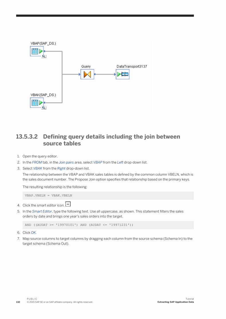
13.5.3.2 Defining query details including the join between source tables
1. Open the query editor.2. In the FROM tab, in the Join pairs area, select VBAP from the Left drop-down list.3. Select VBAK from the Right drop-down list.
The relationship between the VBAP and VBAK sales tables is defined by the common column VBELN, which is the sales document number. The Propose Join option specifies that relationship based on the primary keys.
The resulting relationship is the following:
VBAP.VBELN = VBAK.VBELN
4. Click the smart editor icon. 5. In the Smart Editor, type the following text. Use all uppercase, as shown. This statement filters the sales
orders by date and brings one year's sales orders into the target.
AND ((AUDAT >= '19970101') AND (AUDAT <= '19971231'))
6. Click OK.7. Map source columns to target columns by dragging each column from the source schema (Schema In) to the
target schema (Schema Out).
132P U B L I C© 2015 SAP SE or an SAP affiliate company. All rights reserved.
TutorialExtracting SAP Application Data

Table 34:
Table Column
VBAP VBELN
POSNR
MATNR
NETWR
VBAK KVGR1
AUDAT
8. As shown in the following table, rename the target columns, verify data types, and add descriptions.To change the name or description of a target column, double-click the column name. In the Properties dialog box, type the new column name and description.
Use the following column names, data types, and descriptions:
Table 35:
Original name New name Data type Description
VBELN SLS_doc_no varchar(10) Sales document
POSNR SLS_doc_line_no varchar(6) Sales document line item
MATNR Material_no varchar(18) Material number
NETWR Net_value varchar(15) Order item value
KVGR1 Cust_ID varchar(3) Customer ID
AUDAT SLS_doc_date date Document date
The sales fact table contains a column named ord_status that indicates an order's status. The order status value comes from a table that is not one of the input tables. To implement this, add a column to the output table and map its value by using a function call that looks up the order status value.
13.5.3.3 Adding a column that reflects a value in another table using a lookup
1. In the query editor, right-click the target schema query name and click New Output Column.2. Define the column as follows:
Name: ord_status
Data type: varchar(1)
Description: Order item status
Click OK.3. The order item status comes from a value in the VBUP table. To indicate the correct row and value to populate
the ord_status column, you define a lookup function in the Mapping text box.Click the ord_status column in the target schema.
TutorialExtracting SAP Application Data
P U B L I C© 2015 SAP SE or an SAP affiliate company. All rights reserved. 133
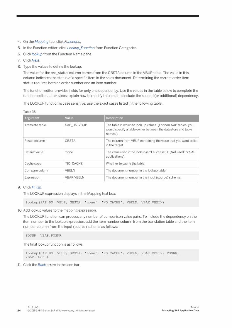
4. On the Mapping tab, click Functions.5. In the Function editor, click Lookup_Function from Function Categories.6. Click lookup from the Function Name pane.7. Click Next.8. Type the values to define the lookup.
The value for the ord_status column comes from the GBSTA column in the VBUP table. The value in this column indicates the status of a specific item in the sales document. Determining the correct order item status requires both an order number and an item number.
The function editor provides fields for only one dependency. Use the values in the table below to complete the function editor. Later steps explain how to modify the result to include the second (or additional) dependency.
The LOOKUP function is case sensitive; use the exact cases listed in the following table.
Table 36:
Argument Value Description
Translate table SAP_DS..VBUP The table in which to look up values. (For non-SAP tables, you would specify a table owner between the datastore and table names.)
Result column GBSTA The column from VBUP containing the value that you want to list in the target.
Default value 'none' The value used if the lookup isn't successful. (Not used for SAP applications).
Cache spec 'NO_CACHE' Whether to cache the table.
Compare column VBELN The document number in the lookup table.
Expression VBAK.VBELN The document number in the input (source) schema.
9. Click Finish.The LOOKUP expression displays in the Mapping text box:
lookup(SAP_DS..VBUP, GBSTA, 'none', 'NO_CACHE', VBELN, VBAK.VBELN)
10. Add lookup values to the mapping expression.The LOOKUP function can process any number of comparison value pairs. To include the dependency on the item number to the lookup expression, add the item number column from the translation table and the item number column from the input (source) schema as follows:
POSNR, VBAP.POSNR
The final lookup function is as follows:
lookup(SAP_DS..VBUP, GBSTA, 'none', 'NO_CACHE', VBELN, VBAK.VBELN, POSNR, VBAP.POSNR)
11. Click the Back arrow in the icon bar.
134P U B L I C© 2015 SAP SE or an SAP affiliate company. All rights reserved.
TutorialExtracting SAP Application Data
13.5.3.4 Defining data transport details
1. Click the name of the data transport object to open its editor.2. Enter the output file name in the File name box:
sales_fact.dat
3. Click Replace File.This truncates the file each time the data flow runs.
4. Click the Back arrow in the icon bar.
13.5.3.5 Defining the order of execution for the data flow
1. Make sure the DF_SAP_SalesFact data flow is open in the workspace.2. Connect the right of the DF_ABAP_SalesFact ABAP data flow to the left of the SALES_FACT table.
13.5.4 Validating the SAP_SalesFact data flow and executing the job
13.5.4.1 Validating and executing
1. With the DF_SAP_SalesFact data flow open in the workspace, click the Validate All button on the toolbar. If your design contains errors, the Output window describes them.
2. As you did in previous exercises, execute the job named JOB_SAP_SalesFact. No error messages should appear in the Output window. You might see a warning message indicating that a conversion from a date to datetime value occurred.
3. Using a DBMS query tool, check the contents of the SALES_FACT table.
13.6 New Terms
Terms examined in this section included:
TutorialExtracting SAP Application Data
P U B L I C© 2015 SAP SE or an SAP affiliate company. All rights reserved. 135

Table 37:
Term Meaning
ABAP data flow A Data Services object that generates ABAP to extract data from SAP application sources.
An ABAP data flow can only be defined in a data flow definition.
Data transport A Data Services object that stores the output of an ABAP data flow.
13.7 Summary
In this section, you have repopulated the following tables from an SAP source:
● Customer dimension● Material dimension● Sales fact
For more information, see the Supplement for SAP.
136P U B L I C© 2015 SAP SE or an SAP affiliate company. All rights reserved.
TutorialExtracting SAP Application Data

14 Running a Real-time Job in Test Mode
Data Services supports real-time data transformation. Real-time means that Data Services can receive requests from ERP systems and Web applications and send replies immediately after getting the requested data from a data cache or a second application. You define operations for processing on-demand messages by building real-time jobs in the Designer.
Data Services real-time jobs have the following characteristics.
● Each real-time job contains a single real-time data flow (RTDF) that runs until explicitly stopped.● Real-time jobs can process requests in XML message format and SAP applications via IDoc format. This
exercise focuses on a simple XML-based example that you will import.● In normal operation, the Data Services Access Server provides a listener that forwards XML requests to the
appropriate real-time job (or "service").● In development, you can run Data Services real-time jobs in test mode from the Designer using XML files
rather than XML messages for the sources and targets.
NoteIf you are unsure whether your Data Services license includes real-time capabilities, contact your sales representative.
For more information about real-time jobs, see the Reference Guide.
14.1 Exercise
This optional exercise imports a real-time job and runs it in test mode. The job transforms the input string Hello World to World Hello.
1. Navigate in your Data Services installation directory to the \ConnectivityTest subdirectory. Copy the files TestOut.dtd, TestIn.dtd, TestIn.xml, and ClientTest.txt to the C:\temp directory.
2. Navigate in your Data Services installation directory to the \bin subdirectory. Copy the file ClientTest.exe to the C:\temp directory.
NoteClientTest.exe uses DLLs in your Data Services\bin directory. If you encounter problems, ensure that you have included Data Services\bin in the Windows environment variables path statement.
3. Start the Designer and log in to your repository.4. Import TestConnectivity.atl: In the object library with any tab selected, right-click in the blank space and
click Repository Import From File . Navigate in your Data Services installation directory to \ConnectivityTest and open TestConnectivity.atl.
TutorialRunning a Real-time Job in Test Mode
P U B L I C© 2015 SAP SE or an SAP affiliate company. All rights reserved. 137
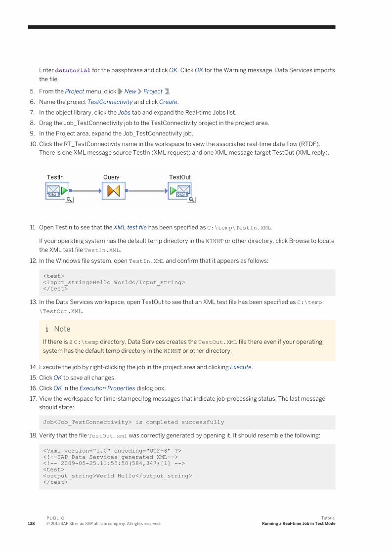
Enter dstutorial for the passphrase and click OK. Click OK for the Warning message. Data Services imports the file.
5. From the Project menu, click New Project .6. Name the project TestConnectivity and click Create.7. In the object library, click the Jobs tab and expand the Real-time Jobs list.8. Drag the Job_TestConnectivity job to the TestConnectivity project in the project area.9. In the Project area, expand the Job_TestConnectivity job.10. Click the RT_TestConnectivity name in the workspace to view the associated real-time data flow (RTDF).
There is one XML message source TestIn (XML request) and one XML message target TestOut (XML reply).
11. Open TestIn to see that the XML test file has been specified as C:\temp\TestIn.XML.
If your operating system has the default temp directory in the WINNT or other directory, click Browse to locate the XML test file TestIn.XML.
12. In the Windows file system, open TestIn.XML and confirm that it appears as follows:
<test> <Input_string>Hello World</Input_string> </test>
13. In the Data Services workspace, open TestOut to see that an XML test file has been specified as C:\temp\TestOut.XML.
NoteIf there is a C:\temp directory, Data Services creates the TestOut.XML file there even if your operating system has the default temp directory in the WINNT or other directory.
14. Execute the job by right-clicking the job in the project area and clicking Execute.15. Click OK to save all changes.16. Click OK in the Execution Properties dialog box.17. View the workspace for time-stamped log messages that indicate job-processing status. The last message
should state:
Job<Job_TestConnectivity> is completed successfully
18. Verify that the file TestOut.xml was correctly generated by opening it. It should resemble the following:
<?xml version="1.0" encoding="UTF-8" ?> <!--SAP Data Services generated XML--> <!-- 2009-05-25.11:55:50(584,347)[1] --><test> <output_string>World Hello</output_string> </test>
138P U B L I C© 2015 SAP SE or an SAP affiliate company. All rights reserved.
TutorialRunning a Real-time Job in Test Mode

19. If the job did not execute successfully, view the error log and troubleshoot as necessary.
TutorialRunning a Real-time Job in Test Mode
P U B L I C© 2015 SAP SE or an SAP affiliate company. All rights reserved. 139

Important Disclaimers and Legal Information
Coding SamplesAny software coding and/or code lines / strings ("Code") included in this documentation are only examples and are not intended to be used in a productive system environment. The Code is only intended to better explain and visualize the syntax and phrasing rules of certain coding. SAP does not warrant the correctness and completeness of the Code given herein, and SAP shall not be liable for errors or damages caused by the usage of the Code, unless damages were caused by SAP intentionally or by SAP's gross negligence.
AccessibilityThe information contained in the SAP documentation represents SAP's current view of accessibility criteria as of the date of publication; it is in no way intended to be a binding guideline on how to ensure accessibility of software products. SAP in particular disclaims any liability in relation to this document. This disclaimer, however, does not apply in cases of wilful misconduct or gross negligence of SAP. Furthermore, this document does not result in any direct or indirect contractual obligations of SAP.
Gender-Neutral LanguageAs far as possible, SAP documentation is gender neutral. Depending on the context, the reader is addressed directly with "you", or a gender-neutral noun (such as "sales person" or "working days") is used. If when referring to members of both sexes, however, the third-person singular cannot be avoided or a gender-neutral noun does not exist, SAP reserves the right to use the masculine form of the noun and pronoun. This is to ensure that the documentation remains comprehensible.
Internet HyperlinksThe SAP documentation may contain hyperlinks to the Internet. These hyperlinks are intended to serve as a hint about where to find related information. SAP does not warrant the availability and correctness of this related information or the ability of this information to serve a particular purpose. SAP shall not be liable for any damages caused by the use of related information unless damages have been caused by SAP's gross negligence or willful misconduct. All links are categorized for transparency (see: http://help.sap.com/disclaimer).
140P U B L I C© 2015 SAP SE or an SAP affiliate company. All rights reserved.
TutorialImportant Disclaimers and Legal Information

TutorialImportant Disclaimers and Legal Information
P U B L I C© 2015 SAP SE or an SAP affiliate company. All rights reserved. 141

www.sap.com/contactsap
© 2015 SAP SE or an SAP affiliate company. All rights reserved.No part of this publication may be reproduced or transmitted in any form or for any purpose without the express permission of SAP SE or an SAP affiliate company. The information contained herein may be changed without prior notice.Some software products marketed by SAP SE and its distributors contain proprietary software components of other software vendors. National product specifications may vary.These materials are provided by SAP SE or an SAP affiliate company for informational purposes only, without representation or warranty of any kind, and SAP or its affiliated companies shall not be liable for errors or omissions with respect to the materials. The only warranties for SAP or SAP affiliate company products and services are those that are set forth in the express warranty statements accompanying such products and services, if any. Nothing herein should be construed as constituting an additional warranty.SAP and other SAP products and services mentioned herein as well as their respective logos are trademarks or registered trademarks of SAP SE (or an SAP affiliate company) in Germany and other countries. All other product and service names mentioned are the trademarks of their respective companies.Please see http://www.sap.com/corporate-en/legal/copyright/index.epx for additional trademark information and notices.
![2012.04.19 - SmartCloud Enterprise - object storage [SmartCloud Services]](https://static.fdocuments.us/doc/165x107/5490ab89b479596a158b458d/20120419-smartcloud-enterprise-object-storage-smartcloud-services.jpg)