• 95 •

DANIEL FERRÉS

BUSINESS CYCLES AND THE CHOICEOF MONETARY POLICY

TARGETS WITH CENTRAL BANKLEARNING

Victor Pacharoni*June 29, 2006

REVISTA DE CIENCIAS EMPRESARIALES Y ECONOMÍA, PP. 95 - 114, AÑO 5 (2006) – UNIVERSIDAD DE MONTEVIDEO

In the “new open economy” macro literature, the role of monetary policy focuses on Taylor rules,with some “stickiness” in price or wage dynamics.However this paper incorporates a “learning” process on the side of the Central Bank. This paperuses a stochastic dynamic general equilibrium model for small open economy, with terms of tradeshocks and different degrees of information stickiness. This paper has produces results showingthat the central bank should target another variable (besides inflation) to improve welfare. Theresult is on based on incomplete pass-through of exchange rate and stickiness in the Central Bank“learning” the true model. However this model has neither labor decisions nor productivity shocks.This model shows that if there are more sources of “noise” in the economy, a second variable in thepolicy function improves welfare.

RESUMEN

En la literatura de la “nueva macroeconomía abierta”, el rol de la política monetaria se enfoca en laregla de Taylor, con precios o salarios “pegajosos”. Sin embargo este artículo incorpora un procesode “aprendizaje” por parte del Banco Central. El trabajo usa un modelo dinámico de equilibriogeneral estocástico para pequeñas economías abiertas, con movimientos en los Términos de Inter-cambio y diferentes tiempos para conocer la información. El resultado de este artículo muestra queel Banco Central debe tener por objetivo otra variable, además de la inflación, para mejorar elbienestar. El resultado está basado en el pasaje incompleto de tasa de cambio y el tiempo en elBanco Central “aprende” el verdadero modelo. Sin embargo este modelo no tiene en cuenta, nidecisiones de trabajo, ni perturbaciones de la productividad. Este modelo muestra que si hay másfuentes de ruido en la economía, una segunda variable en la función de política mejora el bienestar.

ABSTRACT

*Universidad Católica de Córdoba, Argentina. Email: victorp@uccor.edu.ar

• 96 •

BUSINESS CYCLES AND THE CHOICE OF MONETARY POLICY TARGETS WITH CENTRAL BANK LEARNING

INTRODUCTION

In the Real Business Cycle (RBC) approach to open economics, large and recurrent fluctuations interms of trade are widely viewed as an important driving force of business cycles. The terms oftrade affect the industrial countries mainly by raising the relative price of energy. In developingcountries this effect primarily affects the price of imported capital goods.

In the literature of the “new open economy” macro, the role of monetary policy focuses on Taylorrules, with some “stickiness” in price or wage dynamics. However there is another form of stickiness,and that is in the form of “sticky information”. Mankiw and Reis (2002) contend that this form ofstickiness displays properties that are more consistent with accepted views about monetary policythan the commonly used sticky price model. One form of sticky information is when one or moreagent has to “learn” the process of the economy.

Many of the papers in this literature focus on the learning process in the private sector and howthey need to learn the behavior of public sector, specially the central bank policy rule. (Bullard andMetra, 2002, and Orphanides and Willams, 2003). Following Sargent (1999) and Lim and McNelis(2003), this paper incorporates a “learning” process on the side of the central bank. This meansthat the central bank does not know the true “laws of motion” of the macroeconomic variablesgenerated by the private sector.

Asset price booms and busts have been important factors in macroeconomic fluctuations in bothindustrial and developing countries. Developments in asset markets can have a significant impacton both inflation and real economic activity. Bernanke and Gertler (2001) argue that it is appropriatethat the central bank respond to them. However they contend that changes in asset prices shouldaffect monetary policy only to the extent that they affect the central bank’s forecast of inflation.Moreover Cecchetti, Genberg, Lipsky and Wadhwani (2002) argue that the central bank can achievesuperior performance by adjusting its policy instruments not only in response to its forecast offuture inflation and the output gap, but to asset prices as well.

Tobin’s q is used to account for the price of replacement of the capital. Tobin’s q is the ratio of themarket value of an additional unit of capital to its replacement cost. Hayashi (1982) shows that theaverage and the marginal values of capital are identical under neoclassical assumptions. Tobin andBrainard (1977) conjecture that the average and marginal values respond in similar ways to shocks,and the empirical evidence in Abel and Blanchard (1986) appears to support the conjecture. Thestock market indices are the value for the Tobin’s q used in this research.

The specific aim of the paper is to examine the welfare implications of incorporating a second keyvariable output growth or asset price volatility to determine the interest rate policy in a small openeconomy subject to terms of trade shocks with the central bank facing limited information.

This paper examines different scenarios where the central bank applies different policy targets ina stochastic dynamic general equilibrium model subject to terms of trade shocks. The behavior ofthe private sector is consistent with forward-looking rational expectations.

• 97 •

VICTOR PACHARONI

The welfare implications are evaluated in different scenarios according to two different stickinesslevels: first, in the learning process of the central bank, and secondly, in the degree of “pass-through” of the exchange rate.

The central bank needs to learn about the laws of motion of goods prices, output, and asset pricesfrom past data, through least squares regression period by period. Using this information, it updatesthe policy rule by a linear quadratic optimization. The monetary authority is thus “boundedly rational”,in the sense of Sargent (1999), where “bounded” means misspecification of the model and “rational”describes the use of least squares. The other scenario is when the central bank follows an “optimal”Taylor rule for each target. In this case, the central bank uses a rule with optimal weights on pastinflation, growth, and asset prices. The weights are selected to maximize welfare.

Following Lim and McNelis (2003), the “pass-through” of the price of imported goods is determinedaccording to the local currency pricing formulation of Betts and Devereux (2000). This paperanalyzes only two cases, full and low pas-through.

The methodology used here is a combination of parameterized expectation algorithm (used for theprivate sector) with a linear quadratic approach when the central bank updates its forecast in thelearning process. Aruoba, Fernández -Villaverde and Rubio Ramírez (2003) show that polynomialsare better than Finite Elements or perturbation methods when there are large shocks. Duffy andMcNelis (2001), show that the neural network approach gives better approximation than thepolynomials with the same number of parameters, or equivalent accuracy with less parameters.

The next Section describes the model, for the private sector and the monetary authority. Section 3presents equilibrium and dynamic programming formulations. Section 4 describes the parametersand initial conditions. Section 5 presents the results of the simulations and Section 6 concludes.

1 MODEL

The framework of analysis contains two modules - a module which describes the behavior of theprivate sector, and module which describes the behavior of the central bank.

1.1 Private Sector Behavior

There are three parts in this subsection: The first is consumption, derived from the utility function,and the demand side of the economy. The second is production from which I derive investment.The third gives constraints of the representative household-firm, of the government and of thecountry.

1.1.1 Consumption

In this economy, there is a representative agent who lives forever. The preferences are given bymaximizing the welfare, the present value of expected utility given by a composite good, Ct, andsubjective endogenous discount factor, ξt.

• 98 •

The symbol Et is the expectations operator, conditional on informationavailable at time t, while βapproximates the elasticity of the endogenous discount factor, ξt, with respect to the averageconsumption index, C. The endogenous discount factor is due to Uzawa (1968) and Mendoza(1991,1995). The main reason for using the endogenous discounting factor is that it produces wellbehaved dynamics with deterministic stationary equilibria in an open economy.

This paper uses a modified endogenous discount function following Schmitt-Grohé and Uribe (2001).The individual agent’s discount factor does not depend on the agent’s consumption, but rather thediscount factor depends on the average level of past consumption. In equilibrium, the individualconsumption index and the average index are identical, Ct = Ct.With that, the representative agent takes, the endogenous discount factor, as given during themaximization problem.

The composite good has the following structure:

Tradeable, (Cr,t) and non-tradeable, (Cn,t), goods are expressed in Cobb-Douglas unitary-elasticityform where θ is the share in traded goods. Tradeable goods are also expressed in a Cobb-Douglasfunction between exportable, (Cx,t), and importable, (Cm,t), goods where a is the share in exportablegoods. The aggregate consumption expenditure constraints are given by the following equations:

where Pt, Pr,t Pn,t, Px,t and Pm,t are the prices in the economy, in traded, in non-traded, exportableand importable goods respectively. The definition of the real exchange rate,(Zt), and the terms oftrade, (Jt), are

BUSINESS CYCLES AND THE CHOICE OF MONETARY POLICY TARGETS WITH CENTRAL BANK LEARNING

• 99 •

VICTOR PACHARONI

1.1.2 Production

There are two production sectors: export and non-traded. Production of exports, (Yx,t), has a Cobb-Douglas technology:

where Ax,t represents the labour factor productivity term in the production of export goods and Kt isthe amount of capital. The production of non-traded goods, (Yn,t), which is usually in services, isgiven by the labour productivity term, (An,t):

Capital has a depreciation rate, (delta), and evolves according the following identity:

where It represents “net” investment. The “gross” investment is the sum of the “net” investmentplus a quadratic adjustment cost function for accumulation of capital, .The parameter governs the adjustment cost of capital. This specific cost function shows anincreasing marginal cost of investment. This assumption captures the observation that a fasterpace of change requires a greater than proportional rise in installation costs. This function also hasthe advantage of equal marginal and average shadow prices for capital. (see Obstfeld and Roggoff,1996).

1.1.3 Constraints

Agent’s Budget Constraint

The representative household-firm has the following budget constraint:

where there are two different taxes: a fixed proportion of the consumption, , and a sum lump tax, , period by period. The nominal exchange rate, (St), translates the international prices to domesticones. The household-firm may lend to the domestic government and accumulate bonds, (Bt), whichpay the nominal interest rate, (it), given by the central bank. They can also borrow and accumulateinternational assets, (Lt), at the fixed interest rate (i*).

The budget constraint presents an equilibrium between expenditures and profits. The expenditureshows the decision which the representative agent makes between consumption and the change inasset position in each period. The profits are defined as the value of production in exportable and

• 100 •

BUSINESS CYCLES AND THE CHOICE OF MONETARY POLICY TARGETS WITH CENTRAL BANK LEARNING

non-traded goods minus the “gross” investment. In this economy all investment takes place inimported goods, produced overseas, and the costs are paid in importable prices.

Government

In this model, the Government makes expenditures, (Gt), in domestic goods and pays for them withtaxes that it collects from households. The government also has a bond with one period of maturitythat pays a nominal interest rate of it. The government covers its deficit period by period with thebonds and the lump sum taxes.

The agents do not received any utility from the government expenditures.

Country

The value of net exports are equal to the change in international bond holdings as follows:

where Xt is the export production and Mt is the import goods. In aggregate terms export productionis identical to the consumption of the export good plus actual exports. Total importable goods equalthe consumption of the importable goods. The non-traded sector is in en equilibrium between supplyand demand by the households and the government.

The usual no-Ponzi game applies to the evolution of real government debt andforeign assets, namely:

This paper imposes more restrictive asset constraints on the international bond by a penalty functionif the ratio of debt and traded GDP is violated with a value grater than L. Thus, the solution methodavoids a corner solution. The government deficit from the previous period is paid bythe lump sum tax,

• 101 •

VICTOR PACHARONI

Exchange rate pass-through and stickiness

Prices of exports and imports are determined exogenously for a small open economy. This paperassumes that price changes are incompletely passed through in import prices. In domestic currencythese prices are given by:

where ω indicates the degree of pass-through of foreign price changes.

The only shocks explored in this paper come from the terms of trade. Specifically:

where lower lecture cases denote the logarithm of the respective prices. It is assumed that eachprice has a unit root process, in logarithms, with random shocks, (εx*,t) and (εx*,t), independently andidentically distributed with standard deviation σ.

1.2 Monetary Authority

The central bank practices are consistent with optimal control models. It chooses an optimal interestrate reaction function (equation 25), given its loss function equation, following the linear quadraticregulator problem (equation 27), and its perception of the evolution of the state variables (equation27).

This study assumes that the monetary authority does not know the exact nature of the privatesector model, and “learns” and updates the state space model period by period. The learningprocess focuses in the evolution of the state variables, (xt), as a function of its own lags as well asthe changes in the interest rate (∆it),

• 102 •

BUSINESS CYCLES AND THE CHOICE OF MONETARY POLICY TARGETS WITH CENTRAL BANK LEARNING

The control variable ∆it is solved as feedback response to the state variables. The feedback functionh is obtained by solving the linear quadratic regulator problem, as discussed in Sargent (1999). Themaximization of loss function, (Λ), is done since the weights, (λt), are negative.

This paper compares different scenarios of state variables (xt), which are combinations of inflation,growth in Tobin’s q and GDP growth:

where πt = ∆pt, ϕt = ∆qt and ηt = ∆yt are the logarithm annualized changes in the respectivevariable.

To do that, the weights on the loss function are chosen to reflect the central bank’s concerns aboutits policy function, as shown in Table 1:

In the first scenario, with a pure inflation target, the policy calls for no change if the key variable isless than the critical value of the policy target. In the other two scenarios, the central bank putsdifferent weights depending the combination of both targets, as Lim and McNelis (2003).

Corresponding to each scenario, the central bank formulates its optimal interest rate feedback rule.It also acts at time t as if its estimated model for the evolution of the variables is true “forever”, thatthe values of the weights in the loss function are permanently fixed. However central bank “falsifies”its own procedure when it updates the coefficients every period (see Sargent, 1999).

• 103 •

2 Equilibrium and Dynamic Programming Formulations

The competitive equilibrium is defined by stochastic processes Ιt, Kt+1, Ct, Px,t, Pm,t, Pn,t, Lt, Bt ,it , ξt t=0 , where the household optimizes the expected value of consumption (1) subject to thebudget constraint (13). The market clears in non-traded sector given by (18), and the restriction oncapital is satisfied by (12).

The Lagrangean for solving the model is given by:

The variable λt is the familiar Lagrangean multiplier representing the marginal utility of wealth. Theterm qt, known as Tobin’s q, represents the Lagrange multiplier for the evolution of capital- it is the“shadow price” for new capital.

Maximizing the Lagrangean with respect to It, Kt+1,Ct, Lt, Bt, λt,qt, yields the following first orderconditions:

∞

VICTOR PACHARONI

• 104 •

BUSINESS CYCLES AND THE CHOICE OF MONETARY POLICY TARGETS WITH CENTRAL BANK LEARNING

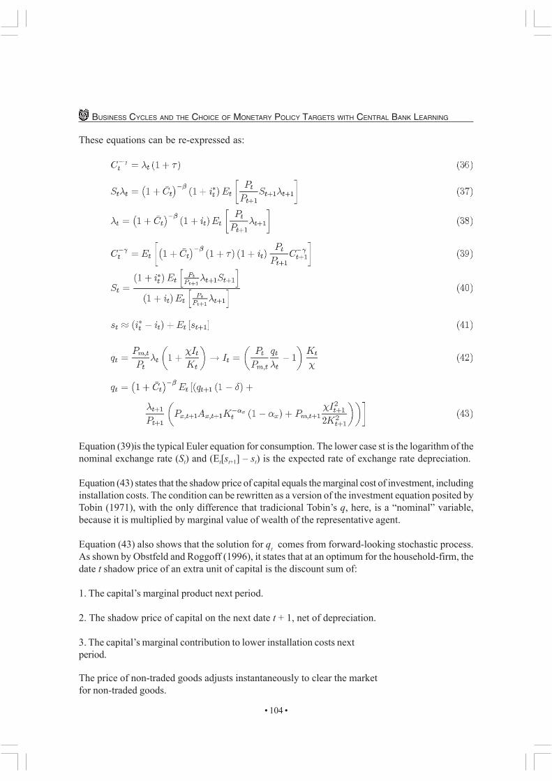
These equations can be re-expressed as:

Equation (39)is the typical Euler equation for consumption. The lower case st is the logarithm of thenominal exchange rate (St) and (Et[st+1] – st) is the expected rate of exchange rate depreciation.

Equation (43) states that the shadow price of capital equals the marginal cost of investment, includinginstallation costs. The condition can be rewritten as a version of the investment equation posited byTobin (1971), with the only difference that tradicional Tobin’s q, here, is a “nominal” variable,because it is multiplied by marginal value of wealth of the representative agent.

Equation (43) also shows that the solution for qt comes from forward-looking stochastic process.As shown by Obstfeld and Roggoff (1996), it states that at an optimum for the household-firm, thedate t shadow price of an extra unit of capital is the discount sum of:

1. The capital’s marginal product next period.

2. The shadow price of capital on the next date t + 1, net of depreciation.

3. The capital’s marginal contribution to lower installation costs nextperiod.

The price of non-traded goods adjusts instantaneously to clear the marketfor non-traded goods.

• 105 •

VICTOR PACHARONI

Thus the model has three “forward-looking” stochastic Euler equations (39), (41) and (43), whichdetermine Ct, St, and qt. These variables, together with rest of the equations, give the solution foreach period with the state of capital and a particular realization of the shocks.

The intra-sectorial consumption decision of the households is solved after the realization of theprices and the total consumption solved intertemporally. The following expressions are the demandfor traded, non-traded, importable and exportable goods as functions of aggregate expenditure, realexchange rate and terms of trade:

The equilibrium set of prices in the model is given by the following equations:

2.1 Parameterized Expectations Algorithm

This subsection studies the parameterized expectations approach to this model. Following Marcet(1988, 1993), Den Haan and Marcet (1990, 1994), and Duffy and McNelis (2001), the approach ofthis study is to “parameterize” the forward-looking expectation in this model, with non-linear functionalforms ψc, ψs, and ψi.

• 106 •

BUSINESS CYCLES AND THE CHOICE OF MONETARY POLICY TARGETS WITH CENTRAL BANK LEARNING

Consumption and nominal exchange rate come from expectation equations (39 and 41), and aretransformed as “parametrized” equations as follow:

The symbol zt-1 represents a vector of observable “instrument” variables known at time t. These“state” variables are: the ratio of initial capital at t, (kt), to its steady state value, (K*), internationalbonds from the last period, (Lt-1), the ratio of the domestic nominal interest rate, (it), to the internationalrate, (i*), and the realization of the international prices of exports, (Px*,t), and imports, (Pf*,t).

The symbol Ωc and Ωs represent the parameters for the expectation function, while ψc and ψs arethe expectation approximation functions.

Combining equations (42) and (43) find investment is a “forward looking” variable, and isparameterized in the following way:

This change has two advantages. First, it places a limitation on the “domain of the expectations”,since the key problem is to find a good set of parameters that will not give a “far away” solution. Asmall deviation on qt implies a large deviation in It. A deviation on It, however, produces smallerdeviations in qt, so using expectations on qt is less efficient. Secondly, working with this variablegives the remaining equations have close form solutions. The combination of these advantages thusgives more accurate and computationally faster solutions.

The functional form for ψt is usually second-order polynomial expansions (see, for example, DenHaan and Marcet, 1994, Schmitt-Groh and Uribe, 2002). However, Duffy and McNelis (2001)have shown that neural networks have produced results with greater accuracy for the same numberof parameters, or equal accuracy with fewer parameters, thanthe second-order polynomial approximation.

The model was simulated for repeated parameter values for Ωc, Ωs and Ωi until convergence wasobtained for the expectation errors and the algorithm found the optimal coefficients Ωc, Ωs and Ωi.In the algorithm, the following non-negativity constraints for consumption and the stocks of capitalfor next period were imposed:

^ ^ ^

• 107 •

VICTOR PACHARONI

3 PARAMETERS AND STEADY STATE

The section discusses the calibration of parameters, initial conditions, and stochastic processes forthe exogenous variables of the model.

3.1 Parameters

The parameter settings for the models appear in Table 2

Many of the parameter selections are common in the literature. The constant relative risk aversionis set at 1.5. The standard deviations of the shocks, σ, on the foreign prices are set at 0.01. Theshares in the traded sector, for exportable goods and in production of exportable good, are equal to0.5. The coefficient β, following Mendoza (1995), is set at 0.009.The adjustment cost scale and depreciation rate are at 0.028 and 0.023 respectively. The tax is10% of the consumption.

This study also uses the following initial conditions: initial bonds domestic and foreign are zeros.Non-traded prices, nominal exchange rate and foreign prices are normalized to 1.

The value of the international interest rate is fixed at 4 percent in annual terms for that in quarterlydata it is one percent.

3.2 Steady State

As usual in General equilibrium models the initial conditions are obtained by the value of steadystate of the variables and value of the parameters. In this model, they are as follows:

• 108 •

BUSINESS CYCLES AND THE CHOICE OF MONETARY POLICY TARGETS WITH CENTRAL BANK LEARNING

• 109 •

VICTOR PACHARONI

4 SIMULATION ANALYSIS

The aim of the simulations is to analyze which is the best policy that the central bank should followunder different economy conditions, “scenarios”.Three central bank policies are analyzed in this study: pure inflation, (π), inflation and growth, (π,η),and inflation and Tobin’s q, (π,ϕ).

The comparison is made in four scenarios. First, the central bank needs to learn the private sectorbehavior and there is a full pass-through of the exchange rate, “Learning, with ω = 1". Second,central bank “learns” private sector behavior and there is a low pass-through “Learning, withω = 0.1". Third, the monetary authority follows an optimal Taylor rule with full pass-through of theexchange rate, “Optimal policy, with ω = 0.1". The fourth has an optimal Taylor rule with low pass-through, “Optimal policy, with ω = 0.1". The values of the pass-through are extreme but for thepurpose of the comparison they are indicative.

The number of simulations, for each scenario and each policy, is 1500 with each containing a time-series of 350 observations.

• 110 •

Figure 1 presents two random realizations of the terms of trade, and the optimal consumption pathsunder different policies in a economy with Taylor rules and low pass-through exchange rate. Therandom walk process followed for international prices produces large fluctuations in terms of tradeprice. It creates large differences in the realizations of the series.

Table 3 presents the mean and standard deviation of these series and their mean after 100 simulations.It shows the large difference between each realization compared with the steady state value for allscenarios (2.02).

The second draw yields a better value than in the steady state. If that is the realization of theeconomy, people are better with the shock than in the steady state. Thus, it is not helpful to compa-re the welfare effect with a “steady state” benchmark. To avoid this problem comparison are doneonly between policies scenarios.

Table 4 presents the value of mean and standard deviation of the sum of welfare function, for thethree policies in the four scenarios. The analytical steady state welfare, by comparison, is -142,12.When it is computed with the same number of observations than the sample its value is -135.0034.

BUSINESS CYCLES AND THE CHOICE OF MONETARY POLICY TARGETS WITH CENTRAL BANK LEARNING

• 111 •

VICTOR PACHARONI

I use a different approach for comparison. For each realization of the shocks the model is solvedfor the 12 different situations (four scenarios and three policies). I then compare welfare effects ofthe central bank policies. The comparisons are in groups of two policies: inflation, (π), versusinflation and growth, (π,η); inflation, (π), versus inflation and Tobin’s q, (ϕ,π); inflation and growth,(π,η), versus inflation and Tobin’s q, (ϕ,π). The left side of Table 5 presents the percentage (with1500 simulations) of each chosen policy. The table was computed with the maximum value betweentwo numbers, the welfare value for each policy. The right side of this table presents the loss if thecentral bank does not follow the policies used in the first column. These values are expressed interms of “percentage of loss” based on the mean of consumption.

For example, for the first scenario "Learning, with ω = 1", inflation policy was chosen 1396 times(93.1%) versus inflation and growth that was chosen only 104 times (6.9%) from 1500 randomrealizations. If it is used the right side of the table, the loss in the consunption is 0.63% when thecentral bank moves from inflation target to inflation and growth targets.The proportions are robust also when they are filtered by removing the "wrong" or "outlier" simulations,in the sense that if a simulation violated the ratio of international bonds allowed in the model or if thesimulation goes to the 5% level of the Marcet statistic (1994), it is removed.

Figure 2:

It is also possible to compare the reaction of the representative agent when the agent faces differentscenarios even with the central bank following the same policy rule. Figure 2 shows the optimalpaths of consumption in different scenarioss for one particular realization under the inflation targetregime. It shows large fluctuations when the central bank follows a “learning” process than if itfollows an optimal Taylor rule. The low pass-through, as expected, gives less welfare than fullpass-through economy.

• 112 •

BUSINESS CYCLES AND THE CHOICE OF MONETARY POLICY TARGETS WITH CENTRAL BANK LEARNING

The results give support for a pure inflation targeting regime. The only exception is for the casewith a lot “noise” in the economy, that is with “sticky” information in the learning process and lowpass-through. Then it is preferable to use a second variable. In this case the second variable isgrowth of output, not the growth of Tobin’s q.

5 CONCLUSION

This paper uses a stochastic dynamic general equilibrium model for small open economy, withterms of trade shocks and different degrees of information stickiness. This paper has producedsome evidence that the central bank should target another variable (besides inflation target) toachieve better welfare.

The argument is on the case where there is incomplete pass-through of exchange rate and themonetary authority faces some stickiness in “learning” the true model. The combination of thesetwo sources of “errors” for the central bank, gives trade-off for policy stances. This result isconsistent with recent results in the literature of “new neoclassical synthesis” in macroeconomics(see Canzoneri, Cumby and Diba, 2002). However this model has neither labor decisions norproductivity shocks. This model shows that if there are more sources of “noise” in the economy, asecond variable in the policy function does improve welfare.There is a clear extension: if there is a productivity shock in the model, will pure inflation targetcontinue to be the optimal policy?

Bibliography

[1] Abel and Blanchard (1986), “The present value of profit and cyclical movements ininvestments”, Econometrica 54 (2).

[2] Auroba, S. Bragan, Jesús Fernández-Villaverde and Juan F. Rubio-Ramírez (2003),“Comparing Solution Methods for Dynamic Equilibrium Economies”, manuscript.

[3] Bernanke, Ben and Mark Gertler (1999), “Monetary Policy and Asset Price volatility. InNew Challenges for Monetary Policy: A Symposium Sponsored by the Federal Reserve Bankof Kansas City”. Federal Reserve Bank of Kansas City.

[4] Bernanke, Ben and Mark Gertler (2001), “Should Central Banks Respond to Movementsin Asset Prices?”, American Economic Review, May.

[5] Betts, Caroline and Michael Devereux (2000), “Exchange Rate Dynamics in a Model ofPricing-to-Market”, Journal of International Economics, 50.

[6] Canzoneri, Matthew B., Robert E. Cumby and Behzad T. Diba (2002), “RecentDevelopments in the Macroeconomic Stabilization Literature: Is Price stability a GoodStabilization strategy?”, Working Paper, Georgetown University, Department of Economics.

• 113 •

VICTOR PACHARONI

[7] Cecchetti Stephen G., Hans Genberg, John Lipsky and Sushil Wadhwani (2002), “Assetprices in a flexible inflation targeting framework”, manuscript.

[8] Den Haan and Albert Marcet (1990), “Solving the Stochastic Growth Model byParametrizing Expectations”, Journal of Business and Economic Statistic 8.

[9] Den Haan and Albert Marcet (1994), “Accuracy in Simulations”, Review of EconomicStudies 61.

[10] Duffy John and Paul McNelis (2001), “Approximating and Simulating the Stochastic GrowthModel: Parameterized Expectations, Neural Networks and the Genetic Algorithm”, Journalof Economics and Control 25.

[11] Hayashi F. (1982), “Tobin’s Marginal q and Average q: A neoclassical interpretation”,Econometrica, Vol. 50.

[12] Lim, G. C. and Paul McNelis (2003), “Central Bank Learning and Stabilization With Com-plete and Partial Pass Through”, manuscript.

[13] Ljungqvist, Lars and Thomas Sargent (2000), Recursive Macroeconomic theory,Cambridge, MA, MIT Press.

[14] Mankiw, N. Gregory and Ricardo Reis (2002), “Sticky Information vs. Sticky Prices: AProposal to Replace the New Keynesian Phillips Curve”, Quarterly Journal of Economics,November.

[15] Marcet Albert (1988), “Solving Nonlinear Models by Parameterizing Expectations”, workingpaper, Graduate School of Industrial Administration, Carnegie Mellon University.

[16] McNelis Paul (2001) “Computational Macrodynamics for Emerging Market Economies”,manuscript, Georgetown University

[17] Mendoza Enrique, (1991), “Real Business Cycles in a Small Open Economy”. AmericanEconomic Review, vol 81 Nº 4.

[18] Mendoza Enrique (1995), “The Terms Of Trade, The Real Exchange Rate, And EconomicFluctuations”. International Economic Review, vol 36 Nº 1.

[19] Obstfeld M., and K. Roggoff (1996), Foundations of International Macroeconomics”,Cambridge, MA, MIT Press.

[20] Sargent, Thomas J. (1999), The Conquest of American Inflation. Princeton, NJ. PrincetonUniversity Press.

[21] Schmitt-Grohé Stephanie, and Martin Uribe (2001), “Closing Small Open EconomyModels”, Journal of International Economics, forthcoming.

• 114 •

BUSINESS CYCLES AND THE CHOICE OF MONETARY POLICY TARGETS WITH CENTRAL BANK LEARNING

[22] Schmitt-Grohé Stephanie, and Martin Uribe (2002), “Solving Dynamic General EquilibriumModels Using a Second-Order Approximation to the Policy Function” manuscript, Universityof Pennsylvania.

[23] Taylor, John B. (1993), “Discretion Versus Policy rules in Practice”, Carnegie-RochasterConference Series on Public Policy, 39.

[24] Tobin J. (1971), “A General Equilibrium Approach to Monetary Theory”, in his Essays inEconomics: Macroeconomics, Vol 1, Chicago.

[25] Tobin J. and W. C. Brainard (1977), “Asset Market and the Cost of Capital”, in BelaBalassa and Richard Nelson, eds., Economic Progress, Private Values and Public Policy:Essays in Honor of William Fellner, Amsterdam.

[26] Walsh Carl E. (2000), Monetary Theory and Policy, Cambridge, MA: MIT Press, 2daedition.

[27] Uzawa, H. (1968), Time Preference, The Consumption Function, and Optimum Asset Hol-dings in J. N. Wolfe, editor, Value, Capital and Growth: Papers in Honor of Sir JohnHicks. Edinburgh: University of Edinburgh Press.