Burning geometric graphs

Arya Tanmay Gupta, 201861003

DissertationFor partial fulfilment of degree

Master of Technology in Computer Science and Engineering

July 2020

Supervisor:Dr. Swapnil A. Lokhande, Assistant Professor

Department of Computer Science and Engineering

Indian Institute of Information Technology Vadodara, India

arX

iv:2

010.

0143

9v1

[cs

.DM

] 3

Oct

202

0

Indian Institute of Information Technology Vadodara

CERTIFICATE

This is to certify that Mr. Arya Tanmay Gupta, Institute ID. 201861003, was astudent of Master of Technology in Computer Science and Engineering at the Instituteduring 2018-2020. He has satisfactorily completed a dissertation on “Burning geometricgraphs” during the year 2019-2020.

Supervisor(Dr. Swapnil A. Lokhande)

PIC/Dean Academics Head of the Department(Dr. Pratikkumar Shah) (Dr. Jignesh S. Bhatt)

INSTITUTE SEAL

ii

Acknowledgements

I thank all the persons who share credit in the completion of the research work, presentedin this dissertation, at the Indian Institute of Information technology Vadodara (IIITV).

I thank Dr. Swapnil A. Lokhande (Assistant Professor, IIIT Vadodara, India) tosupervise my work at IIITV and to give useful comments in order to improve my work andpresentation.

I thank Dr. Kaushik Mondal (Assistant Professor, Indian Institute of TechnologyRopar, India), who unofficially supervised my study. I thank him for his continuous support,help, and guidance, which was given to me not only to help me in my study, but also to helpme during general life scenarios in various aspects, also from the perspective of my researchcareer. His sincere efforts reduced the labour that I would have to input otherwise. I feelhonoured to work under the supervision of a personality such as himself.

I must thank Prof. S. K. Patra (Director, IIITV, India) and other members of admin-istration to support my research at the Indian Institute of Information Technology Vadodara.

I thank my students at IIITV and my colleagues who kept me motivated all along.I thank my parents, and almighty god.

Arya Tanmay Gupta

iii

Contents

List of Figures vii

List of Tables ix

Abstract 1

1 Introduction 21.1 Origin, etymology, history . . . . . . . . . . . . . . . . . . . . . . . . . . . . 21.2 Graphs . . . . . . . . . . . . . . . . . . . . . . . . . . . . . . . . . . . . . . . 31.3 Decision Problems . . . . . . . . . . . . . . . . . . . . . . . . . . . . . . . . 41.4 Languages . . . . . . . . . . . . . . . . . . . . . . . . . . . . . . . . . . . . . 41.5 Algorithms . . . . . . . . . . . . . . . . . . . . . . . . . . . . . . . . . . . . . 51.6 Easy and Hard problems . . . . . . . . . . . . . . . . . . . . . . . . . . . . . 51.7 Strong NP-Completeness . . . . . . . . . . . . . . . . . . . . . . . . . . . . . 6

1.7.1 Brute force . . . . . . . . . . . . . . . . . . . . . . . . . . . . . . . . 61.7.2 Weak sense . . . . . . . . . . . . . . . . . . . . . . . . . . . . . . . . 7

1.8 Turing reduction . . . . . . . . . . . . . . . . . . . . . . . . . . . . . . . . . 81.9 Approximation, approximability and inapproximability . . . . . . . . . . . . 81.10 Main objectives . . . . . . . . . . . . . . . . . . . . . . . . . . . . . . . . . . 91.11 Organization of the chapters . . . . . . . . . . . . . . . . . . . . . . . . . . . 9

2 Preliminaries 112.1 Complexity notation functions . . . . . . . . . . . . . . . . . . . . . . . . . . 112.2 Definitions for symbols . . . . . . . . . . . . . . . . . . . . . . . . . . . . . . 112.3 Problems in NP . . . . . . . . . . . . . . . . . . . . . . . . . . . . . . . . . . 132.4 Graph Classes . . . . . . . . . . . . . . . . . . . . . . . . . . . . . . . . . . . 14

2.4.1 Spider graphs . . . . . . . . . . . . . . . . . . . . . . . . . . . . . . . 142.4.2 Pk-free graphs . . . . . . . . . . . . . . . . . . . . . . . . . . . . . . . 142.4.3 Cographs . . . . . . . . . . . . . . . . . . . . . . . . . . . . . . . . . 142.4.4 Disk Graphs . . . . . . . . . . . . . . . . . . . . . . . . . . . . . . . . 152.4.5 Interval Graphs . . . . . . . . . . . . . . . . . . . . . . . . . . . . . . 152.4.6 Permutation graphs . . . . . . . . . . . . . . . . . . . . . . . . . . . . 172.4.7 Split graphs . . . . . . . . . . . . . . . . . . . . . . . . . . . . . . . . 18

iv

3 Literature Survey 193.1 Graph burning . . . . . . . . . . . . . . . . . . . . . . . . . . . . . . . . . . 193.2 Cographs . . . . . . . . . . . . . . . . . . . . . . . . . . . . . . . . . . . . . 193.3 Disk graphs . . . . . . . . . . . . . . . . . . . . . . . . . . . . . . . . . . . . 193.4 Interval graphs . . . . . . . . . . . . . . . . . . . . . . . . . . . . . . . . . . 20

3.4.1 Similarity between a path and an interval graph . . . . . . . . . . . . 203.5 Permutation graphs . . . . . . . . . . . . . . . . . . . . . . . . . . . . . . . . 213.6 Split graphs . . . . . . . . . . . . . . . . . . . . . . . . . . . . . . . . . . . . 21

4 Graph burning: Problem statement 224.1 Introduction . . . . . . . . . . . . . . . . . . . . . . . . . . . . . . . . . . . . 224.2 The underlying problem . . . . . . . . . . . . . . . . . . . . . . . . . . . . . 224.3 Verification of a burning sequence . . . . . . . . . . . . . . . . . . . . . . . . 254.4 Related problems and games . . . . . . . . . . . . . . . . . . . . . . . . . . . 25

4.4.1 Firefighter problem . . . . . . . . . . . . . . . . . . . . . . . . . . . . 254.4.2 Firefighter reserve problem . . . . . . . . . . . . . . . . . . . . . . . . 254.4.3 Graph cleaning . . . . . . . . . . . . . . . . . . . . . . . . . . . . . . 264.4.4 Graph bootstrap percolation . . . . . . . . . . . . . . . . . . . . . . . 26

4.5 Overview of possible applications . . . . . . . . . . . . . . . . . . . . . . . . 264.6 Computational limitations . . . . . . . . . . . . . . . . . . . . . . . . . . . . 274.7 Summary of this chapter . . . . . . . . . . . . . . . . . . . . . . . . . . . . . 27

5 The burning process in graphs 285.1 Burning a simple path or cycle . . . . . . . . . . . . . . . . . . . . . . . . . . 28

5.1.1 Burning a path (or a cycle) of infinite length . . . . . . . . . . . . . . 285.1.2 Governing dynamics . . . . . . . . . . . . . . . . . . . . . . . . . . . 30

5.2 Optimal burning of some general graphs . . . . . . . . . . . . . . . . . . . . 315.3 Algorithm for burning general graphs optimally . . . . . . . . . . . . . . . . 345.4 Summary of this chapter . . . . . . . . . . . . . . . . . . . . . . . . . . . . . 34

6 Other games and problems 356.1 Distinct 3-partition problem . . . . . . . . . . . . . . . . . . . . . . . . . . . 356.2 Firefighter problem . . . . . . . . . . . . . . . . . . . . . . . . . . . . . . . . 356.3 Firefighting general graphs . . . . . . . . . . . . . . . . . . . . . . . . . . . . 376.4 Summary of this chapter . . . . . . . . . . . . . . . . . . . . . . . . . . . . . 37

7 Why is burning hard? 387.1 Burning interval graphs . . . . . . . . . . . . . . . . . . . . . . . . . . . . . . 38

7.1.1 Similarity in burning paths and interval graphs . . . . . . . . . . . . 387.1.2 Interval graph construction for NP-completeness . . . . . . . . . . . . 397.1.3 Example construction . . . . . . . . . . . . . . . . . . . . . . . . . . . 407.1.4 NP-Completeness . . . . . . . . . . . . . . . . . . . . . . . . . . . . . 40

7.2 Burning permutation graphs . . . . . . . . . . . . . . . . . . . . . . . . . . . 437.2.1 Permutation graph construction for NP-completeness . . . . . . . . . 437.2.2 Example construction . . . . . . . . . . . . . . . . . . . . . . . . . . . 447.2.3 NP-Completeness . . . . . . . . . . . . . . . . . . . . . . . . . . . . . 44

7.3 Burning disk graphs . . . . . . . . . . . . . . . . . . . . . . . . . . . . . . . 44

v

7.3.1 Disk graph construction for NP-completeness . . . . . . . . . . . . . 447.3.2 Example construction . . . . . . . . . . . . . . . . . . . . . . . . . . . 457.3.3 NP-Completeness . . . . . . . . . . . . . . . . . . . . . . . . . . . . . 46

7.4 Corollary NP-Hard results . . . . . . . . . . . . . . . . . . . . . . . . . . . . 477.4.1 Burning trees with maximum degree 3 . . . . . . . . . . . . . . . . . 477.4.2 Burning chordal graphs . . . . . . . . . . . . . . . . . . . . . . . . . . 477.4.3 Burning planar graphs . . . . . . . . . . . . . . . . . . . . . . . . . . 477.4.4 Burning bipartite graphs . . . . . . . . . . . . . . . . . . . . . . . . . 477.4.5 Burning path forests . . . . . . . . . . . . . . . . . . . . . . . . . . . 477.4.6 Burning spider graphs . . . . . . . . . . . . . . . . . . . . . . . . . . 477.4.7 Burning forests . . . . . . . . . . . . . . . . . . . . . . . . . . . . . . 477.4.8 NP-Completeness of general graph burning . . . . . . . . . . . . . . . 48

7.5 Summary of this chapter . . . . . . . . . . . . . . . . . . . . . . . . . . . . . 48

8 Easy burning subproblems 498.1 Burning path or cycle (already discussed) . . . . . . . . . . . . . . . . . . . . 498.2 Burning split graphs . . . . . . . . . . . . . . . . . . . . . . . . . . . . . . . 49

8.2.1 Burning connected split graphs . . . . . . . . . . . . . . . . . . . . . 498.2.2 Burning general split graphs . . . . . . . . . . . . . . . . . . . . . . . 50

8.3 Burning cographs . . . . . . . . . . . . . . . . . . . . . . . . . . . . . . . . . 518.4 Summary of this chapter . . . . . . . . . . . . . . . . . . . . . . . . . . . . . 51

9 Approximating the burning sequence 529.1 Approximation for general graphs . . . . . . . . . . . . . . . . . . . . . . . . 529.2 How close can we approximate? . . . . . . . . . . . . . . . . . . . . . . . . . 539.3 Approximating the burning of connected interval graphs . . . . . . . . . . . 569.4 Summary of this chapter . . . . . . . . . . . . . . . . . . . . . . . . . . . . . 57

10 Conclusion and future work 5810.1 Observations . . . . . . . . . . . . . . . . . . . . . . . . . . . . . . . . . . . . 58

10.1.1 On graph burning . . . . . . . . . . . . . . . . . . . . . . . . . . . . . 5810.1.2 Burning versus other problems . . . . . . . . . . . . . . . . . . . . . . 5810.1.3 Approximating the burning sequence . . . . . . . . . . . . . . . . . . 58

10.2 What next? . . . . . . . . . . . . . . . . . . . . . . . . . . . . . . . . . . . . 5910.2.1 Discrete mathematics and theoretical algorithm design . . . . . . . . 5910.2.2 Practical implementations . . . . . . . . . . . . . . . . . . . . . . . . 59

Bibliography 60

vi

List of Figures

1.1 An example of unweighted graph. Entities are represented as vertices p, q, r, ..., wand there is an edge between a pair of vertices if the corresponding edges arerelated as per some relation function. The weight associated to the pair (s, u),for example, is 1, and the weight associated to the pair (u,w) is 0. . . . . . . 3

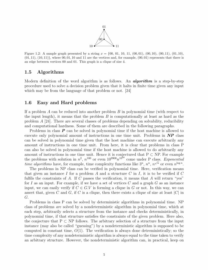
1.2 A sample graph presented by a string x = 00, 01, 10, 11, (00, 01), (00, 10),(00, 11), (01, 10), (01, 11), (10, 11), where 00, 01, 10 and 11 are the verticesand, for example, (00, 01) represents that there is an edge between vertices 00and 01. This graph is a clique of size 4. . . . . . . . . . . . . . . . . . . . . . 5

1.3 Classification of algorithms / problems based on runtime complexity. . . . . 6

2.1 An example spider graph. . . . . . . . . . . . . . . . . . . . . . . . . . . . . 142.2 a: a single vertex is a cograph; b: a disjoint union of two copies of the cograph

in (a) is a cograph; c: a complete join of two copies of the cograph in (b) is acograph; d: a disjoint union of the cographs in (b) and (c) is a cograph; e: thegraph complement of the cograph in (d) is a cograph. . . . . . . . . . . . . . 15

2.3 (a) arrangement of disks and (b) the corresponding disk graph, geometricallynot according to the arrangement of the disks, but connections according tothe overlap of respective disks. . . . . . . . . . . . . . . . . . . . . . . . . . . 16

2.4 Central disk C ′ and a set of Cir = c1, c2, ..., cq disks with their circumferencetouching the circumference of C ′, and not overlaping with each other, or withC ′ . . . . . . . . . . . . . . . . . . . . . . . . . . . . . . . . . . . . . . . . . 16

2.5 An example set of intervals (a) and the corresponding interval graph (b). . . 172.6 Positions of the vertical line while traversing an example set on intervals on

the real line. This figure presents each frame where a new untraversed intervalis encountered and a clique in the graph (in Figure 2.5-(b)) is added. . . . . 17

2.7 Representation of permutation graph corresponding to (O,P ), where O =(1, 2, 3, 4, 5, 6, 7, 8) and P = (3, 1, 5, 2, 7, 4, 8, 6). . . . . . . . . . . . . . . . . . 17

2.8 An example split graph. C = v1, v2, . . . , v5 is the clique and I = v6, v7, . . . , v10is the independent set excerpt of this split graph. . . . . . . . . . . . . . . . 18

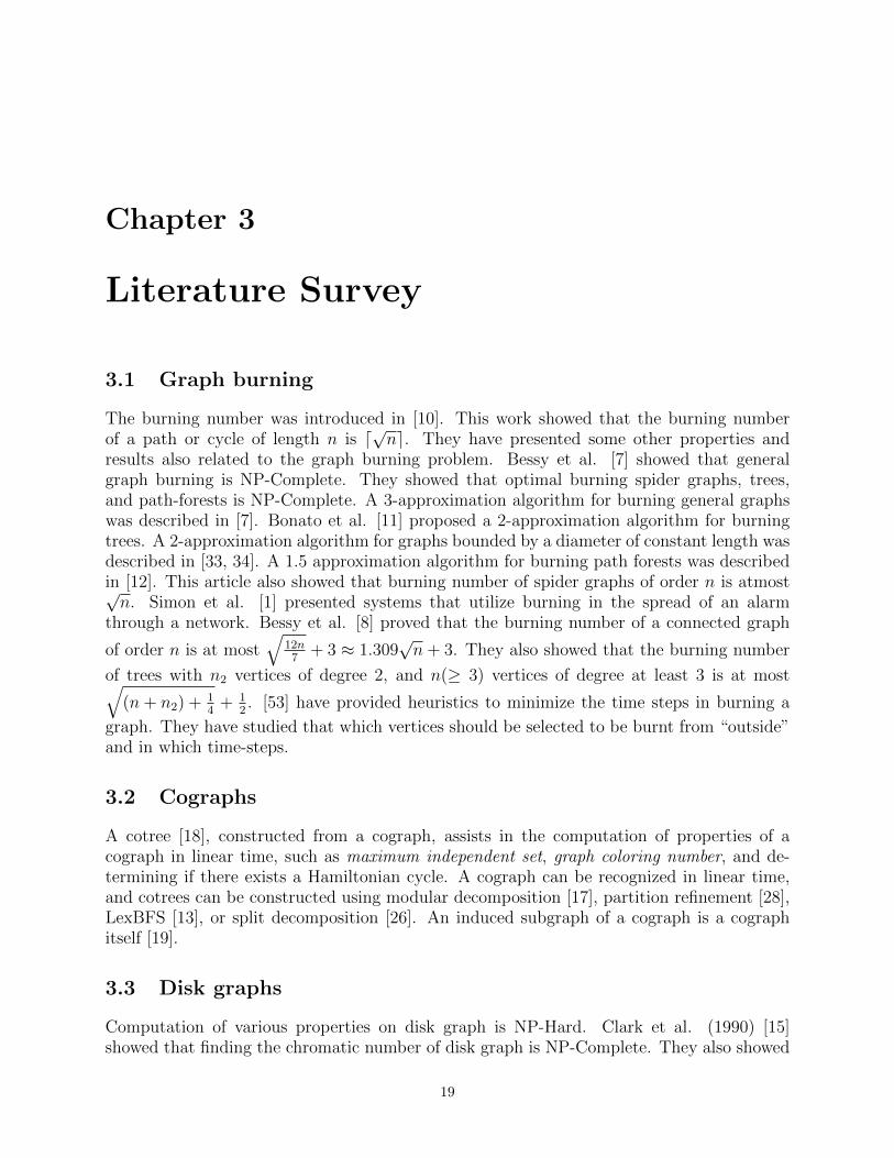
3.1 Demonstration of what happens if we try to create an interval graph cycleand the corresponding set of intervals. The dotted lines are the prospectiveedges which shall form, apart from the original cycle of k vertices. Either orboth of the terminal vertices v1 or vk, on the original path v1, ..., vk shall beconnected to all the vertices from v2, v3, . . . , vk−1. . . . . . . . . . . . . . . . 21

vii

4.1 Burning a graph. See that part b does not run in step 1 because there is novertex that was burnt before step 1, so the fire did not spread. Once we labelthe vertex in some step, we do not change the label in any future steps. . . . 23

4.2 (Better) Burning procedure (optimal) on an example graph. The subjectgraph is same as that on which an arbitrary burning procedure is demonstratedin Figure 4.1. . . . . . . . . . . . . . . . . . . . . . . . . . . . . . . . . . . . 24

5.1 Burning process on a path of ∞ length; the fire sources are placed at ∞distance from each other. . . . . . . . . . . . . . . . . . . . . . . . . . . . . . 29

5.2 Burning of a path of 9 vertices (optimal procedure). The vertices are markedby the step number in which they are burned. For each step, the vertex whichis selected (arbitrarily) as a victim to be burned (the fire source) is marked bya , and those which are burned by the fire spread from already burned verticesare marked by b. . . . . . . . . . . . . . . . . . . . . . . . . . . . . . . . . . 30

5.3 Optimal burning of SP (3, 4). . . . . . . . . . . . . . . . . . . . . . . . . . . 325.4 Optimal burning of SP (4, 4) . . . . . . . . . . . . . . . . . . . . . . . . . . 325.5 Optimal burning of a graph SP (d, k′ − 1), where d ≥ k′ + 1. S ′SP (d,k′−1) =

(y1, y2, ..., yk′) is the optimal burning sequence. . . . . . . . . . . . . . . . . . 335.6 Optimal burning of a graph GSP with k′ connected components, where GSP =

SP (d1, 0) ∪ SP (d2, 1) ∪ SP (d3, 2) ∪ ... ∪ SP (dk′ , k′ − 1) and di ≥ i+ 1. . 34

7.1 Structure of a Tj with 33 vertices, along with the extra vertices connected toit. The dashed line represents the fact that other subpaths may be connectedto a Tj on either or both ends. . . . . . . . . . . . . . . . . . . . . . . . . . . 39

7.2 Construction of example IG(X). . . . . . . . . . . . . . . . . . . . . . . . . 417.3 Construction of example DK(X). . . . . . . . . . . . . . . . . . . . . . . . . 46

8.1 If the first fire source is placed on i, then the burning sequence is i, c1, c2. If,otherwise, the first fire source is placed on c1 (for example), then the burningsequence is c1, i . . . . . . . . . . . . . . . . . . . . . . . . . . . . . . . . . . 50

9.1 Burning of a graph with k′ components compi. Each compi having one centralhead vertex, has di ≥ i+ 1 arms of equal length i− i. Burning number of thisgraph is k′. . . . . . . . . . . . . . . . . . . . . . . . . . . . . . . . . . . . . 55

9.2 Burning of a graph with k′ components compi. Each compi having one centralhead vertex, has di ≥ i+ 1 arms of equal length i− i. A burning sequence oflength 3k′ − 3 is shown to not to be able to burn SP (X) completely. . . . . 55

viii

List of Tables

5.1 Step-wise number of burned vertices in all the clusters Ci in a path of infinitelength, as shown in figure 1. Total burning vertices shown at bottom left. . . 28

ix

Abstract

A procedure called graph burning was introduced to facilitate the modelling of spread of analarm, a social contagion, or a social influence or emotion on graphs and networks.

Graph burning runs on discrete time-steps (or rounds). At each step t, first (a) anunburned vertex is burned (as a fire source) from “outside”, and then (b) the fire spreads tovertices adjacent to the vertices which are burned till step t− 1. This process stops after allthe vertices of G have been burned. The aim is to burn all the vertices in a given graph inminimum time-steps. The least number of time-steps required to burn a graph is called itsburning number. The less the burning number is, the faster a graph can be burned.

Burning a general graph optimally is an NP-Complete problem. It has been proved thatoptimal burning of path forests, spider graphs, and trees with maximum degree three is NP-Complete. We study the graph burning problem on several sub-classes of geometric graphs.

We show that burning interval graphs (Section 7.1, Theorem 7.1), permutation graphs(Section 7.2, Theorem 7.2) and disk graphs (Section 7.3, Theorem 7.3) optimally is NP-Complete. In addition, we opine that optimal burning of general graphs (Section 9.2, Con-jecture 9.1) cannot be approximated better than 3-approximation factor.

1

Chapter 1

Introduction

In this chapter, we discuss some fundamentals related to our subject problem. We discusswhat are graphs, what are decision problems and languages in computing theory. We discussabout some interesting facts about the word “algorithm”, and further when we have discussedenough background details, we describe algorithms formally as per the current perspective.We discuss how we differ between easy and hard problems, along with a brief description ofwhat NP, NP-Complete and NP-Hard problems are. We also briefly discuss the reducibilityof certain problems into one-another, and the approximability of hard problems.

1.1 Origin, etymology, history

Lionardo Pisano [52], more popularly known as Fibonacci, introduced the traditionalIndian mathematical methods to Europe in the 13th century. Until then, abacus was usedto perform all calculations. Pisano introduced a mathematics which was more efficient:computations could be performed on numbers without bounds on their digit-length. Aperson who could perform computations without the use of abacus was called Maestro-de-abaci. And the Europeans started to call this new form of mathematics, which could beperformed on “paper” without abacus, algorithms .

Since then, numerous efforts have been made to translate human intelligence and com-puting ability into artificial machinery. Blaise Pascal [20] built a machine in the 17th

century which could perform addition and subtraction. Gottfried Wilhelm Leibnizbuilt a machine, during the same time, which could perform multiplication and division aswell. Charles Babbage built the famous Difference Engine which could do similar com-putations “automatically”, that is, once the input numbers are supplied to it, it was ableto do the computation without any human intervention. This machine was able to preparetables: it was able to compute polynomials of degree 2 for consecutive integers; this wascalled the method of differences. Babbage built the first prototype of this machine in 1822.

Luigi Frederico Menabrea explained with reference to the Difference Engine thatit was limited only to one type of computations, it could not be applied to solve numerousother problems in which mathematicians might be interested. This led Charles Babbage todesign the Analytical Engine, which could solve the full range of algebraic problems. Thegenerality of the Analytical Engine is discussed in Menabrea’s Italian article Sketch of theAnalytical Engine (1842). It was translated into English by Augustus Ada [44].

Augustus Ada, countess of Lovelace, proposed that the Babbage’s design could be

2

p q

r st

uv

w

Figure 1.1: An example of unweighted graph. Entities are represented as vertices p, q, r, ..., w and there isan edge between a pair of vertices if the corresponding edges are related as per some relation function. Theweight associated to the pair (s, u), for example, is 1, and the weight associated to the pair (u,w) is 0.

used to compute function of any number of functions. On Babbage’s request, she wrotesome additional notes to her “memoir”, most famous one of them is the Note G , in which,firstly, she anticipated an issue: whether computers can exhibit “intelligence”, or, “originalthought”, and secondly, in this note she wrote a sequence of operations (an algorithm) tocompute Bernoulli numbers on the Analytical Engine.

After some decades, Alan Mathison Turing worked on construction of formal lan-guages for any function (or a decision problem, as he presents in [54]). He initiated thedesign of what we call the Turing Machine which works on these formal languages to com-pute for any decision problem. We discuss decision problems and formal languages in thischapter; we do not touch the Turing Machine, the reader is advised to refer [54, 24] to studythe Turing Machine in detail. We start with a brief discussion on graphs, on which thefollowing chapters are majorly based.

1.2 Graphs

A graph is a representation of entities and their relations: generally, a graph tells whichentities are related (unweighted graph); sometimes the relations may have some associatedcost or weightage (weighted graphs). Formally, a graph is a mathematical object whichrepresents entities as vertices, and edges as relations between those vertices: if two entitiesare related, then there will be an edge between the corresponding vertices in the graph. Here,we only discuss relations which are symmetric (if a is related to b, then b is related to a). Sothe edges are bidirectional; we do not show any directions for brevity.

Any cost or weightage related to a relation between a pair of entities is presented as weightson the edges. For example, if two computers are connected in a network, we can denote thefrequency of communication between them in that network as a weight on the edge betweentheir corresponding vertices in the graph representation of that network. Throughout thefollowing chapters, we assume that all the edges have same weight; we consider the weighton all edges to be 1, which we do not show explicitly for brevity; the value of the weight isto represent merely that a given pair of vertices are connected; there are only two weightsassociated with all the pairs of vertices which, 0 or 1, if otherwise the weight associated withsome pair of vertices 0, then we assume that they are not connected. If the vertices a andb are connected, then the weight associated to the pair (a, b) is 1, and if the vertices a andb are connected, then the weight associated to the pair (a, b) is 0. A rough example of anunweighted graph is presented in Figure 1.1.

3

There are various problems which are related to graphs, most of them are computationally“hard” to solve on arbitrary graph inputs. In the following paragraphs, we discuss thedescription of the nature of problems in general, especially the problems which are hard. Weshall keep all the descriptions close to the perspective of graphs: our main focus is on theproblems which are related to graphs.

1.3 Decision Problems

Refer to the problems described under Section 2.3 in Chapter 2. The problems like the graphisomorphism problem, whose solution is either “yes” or “no” are called decision problems.The distinct 3-partition problem is also a decision problem. Other problems such as thelargest clique problem, minimum dominating set problem, largest independent set problem,minimum vertex cover problem, graph coloring problem are optimization problems; they canalso be converted into their respective equivalent decision problem versions. Also, we canadd a mathematical bound B as an additional parameter to a decision problem and andreformulate it. For example we can ask that given a graph G with degree bound B, doesthere exist a clique of size at least k.

The optimization problems are at least as hard as decision problems problems. Forexample, if we can compute the largest clique in G, we can also compute if there exists aclique in G whose size is at least k. Hardness of many decision problems is closely tied to theircorresponding optimization versions [24]. For example, decision version of the clique problemis no easier than the optimization version of the problem. Likewise, we can transform anyproblem into its corresponding decision version.

1.4 Languages

Let that x is a sequence of symbols such that a particular decision problem A returns “yes”as output. The language L of a decision problem A is the set of sequences of symbolsfor such that for each sequence in that set, A returns “yes” as output, given the alphabet,and an encoding scheme. For example, let the alphabet be Λ = ‘0’, ‘1’, ‘(’, ‘)’, ‘,’. Let agraph G be represented by an input string x = 00, 01, 10, 11, (00, 01), (00, 10), (00, 11),(01, 10), (01, 11), (10, 11) constructed from Λ. In x, 00, 01, 10 and 11 are the vertices and,for example, (00, 01) represents that there is an edge between vertices 00 and 01. Let e bethe encoding scheme, for example, used to encode G into x. Similarly, we can represent anygraph using the alphabet Λ and the encoding e. Observe that in e, there is no unnecessarypadding of symbols. All such encoding schemes which do not allow any unnecessary paddingof symbols can represent any object (for example, G) with sequences whose lengths arepolynomially bound to one another [24].

Let there be a problem A as follows, given a graph as input, the task is to find if thereis a clique of size at least 4 in that graph. Observe that x represents a graph which isa clique of size 4, as presented in Figure 1.2. x is an element of LA, the language of Aunder the encoding scheme e. LA contains all the possible sequences from the alphabet Λ(under the encoding scheme e) for which A returns ”yes”. A and LA, for example, can beused interchangeably, and similarly, any decision problem with its corresponding languagebecause they are computationally equivalent.

4

00

01

10 11

Figure 1.2: A sample graph presented by a string x = 00, 01, 10, 11, (00, 01), (00, 10), (00, 11), (01, 10),(01, 11), (10, 11), where 00, 01, 10 and 11 are the vertices and, for example, (00, 01) represents that there isan edge between vertices 00 and 01. This graph is a clique of size 4.

1.5 Algorithms

Modern definition of the word algorithm is as follows. An algorithm is a step-by-stepprocedure used to solve a decision problem given that it halts in finite time given any inputwhich may be from the language of that problem or not. [24]

1.6 Easy and Hard problems

If a problem A can be reduced into another problem B in polynomial time (with respect tothe input length), it means that the problem B is computationally at least as hard as theproblem A [24]. There are several classes of problems depending on solvability, reducibilityand computational hardness. Some of them are described in the following paragraphs.

Problems in class P can be solved in polynomial time if the host machine is allowed toexecute only polynomial amount of instructions in one time unit. Problems in NP classcan be solved in polynomial time given that the host machine can execute arbitrarily anyamount of instructions in one time unit. From here, it is clear that problems in class Pcan also be solved in polynomial time if the host machine is allowed to do arbitrarily anyamount of instructions in one time unit. Hence it is conjectured that P ⊂ NP. For examplethe problems with solution in n2, n100 or even 109900n1099 come under P class. Exponentialtime algorithms have, for example, time complexity functions like 3n, nn, n

√n or even nlogn.

The problems in NP class can be verified in polynomial time. Here, verification meansthat given an instance I for a problem A and a structure C in I, it is to be verified if Cfulfils the constraints of A. If C passes the verification, it means that A will return “yes”for I as an input. For example, if we have a set of vertices C and a graph G as an instanceinput, we can easily verify if C ∈ G.V is forming a clique in G or not. In this way, we canassert that, given C and G, if C is a clique, then there exists a clique of size at least |C| inG.

Problems in class P can be solved by deterministic algorithms in polynomial time. NPclass of problems are solved by a nondeterministic algorithm in polynomial time, which ateach step, arbitrarily selects a structure from the instance and checks deterministically, inpolynomial time, if that structure satisfies the constraints of the given problem. Here also,the conjecture that P ⊂ NP follows. The arbitrary selection of a structure from the inputinstance (may also be called “guessing”) by a nondeterministic algorithm is supposed to becomputed in constant time, O(1). The verification is always done detreministically; so thetime complexity of any nondeterministic algorithm is always equal to the time taken to verifyan arbitrary structure. However, the nondeterministic algorithm can, in practical, keep on

5

NP

P

NPC

NPH

Figure 1.3: Classification of algorithms / problems based on runtime complexity.

guessing structures indefinitely and never terminate.NP-Complete is a class of problems to which each problem in NP can be reduced into

in polynomial time. The problems which come in NP-Complete class are also reducible toeach other in polynomial time. NP-Complete problems are are the hardest problems of NPclass.

NP-Hard problems are the problems that are at least as hard as any problem in NP;they may or may not be in NP. So the NP-Complete problems are a subset of NP-Hard prob-lems. In fact, considering the hardness, the NP-Complete problems come in the intersectionbetween NP and NP-Hard problems, as shown in Figure 1.3.

These classifications arise because we are still not able to determine whether the problemsin NP can be solved in polynomial time only, using some algorithm, that is, we still do nothave a mathematical proof as to whether P = NP or not. These classifications are basedon the conjecture that P 6= NP . There are numerous other classes of problems, whichhierarchically allow problems of more complex bounds of time complexity; apart from this,problems can also be classified on the basis of the “extra” space they require for computation.We do not discuss those classes of problems; such problems are discussed in detail in [24]and other works.

1.7 Strong NP-Completeness

Let there be a problem B and n be the length of an arbitrary input x to B. A problem Bis NP-Complete (or NP-Hard) in the strong sense if it remains NP-Complete (or NP-Hard)even when its parameters are bounded by a polynomial p of n.

To prove that a problem B is NP-Complete (or NP-Hard) in the strong sense, we needto show [24] that for some polynomial p, Bp (B constrained by p of n) is NP-Complete (orNP-Hard).

1.7.1 Brute force

A brute force algorithm is an algorithm which tries all possibilities and then compares theoutput of each possibility to produce one possibility as an optimal result. For example,considering the rod cutting problem (see the definition in Section 2.3), an algorithm whichuses brute force to compute the optimal cuts on the rod to produce maximum profit, hastime complexity exponential in the length of rod. We can rather use a dynamic programming

6

approach, on the other hand, to solve any arbitrary rod cutting instance optimally in timequadratic in the length of the rod [16].

Still, there are numerous problems which do not have a solution algorithm (yet) whichruns in polynomial time. Some of the popular examples of such problems are finding thelargest clique, coloring with minimum colors, finding maximum independent set, findingminimum vertex cover in an arbitrary graph. Such problems are yet NP-Hard becausewe have to try and search on every possibility. One of the reasons that these problemshave no solution algorithm which gets executed in polynomial time because no overlappingsubproblems have been defined (so far) for general graphs so that we could use a commondynamic programming approach and reduce the time complexity.

A pseudo-polynomial algorithm is defined for number problems (we discuss examples ofnumber problems shortly). A pseudo- polynomial algorithm runs in time polynomial in thevalue of the the input, rather than the input length. We generally use dynamic programmingapproach to design a pseudo-polynomial time algorithm. Observation 1.1 is stated in [24].

Observation 1.1. If a problem B is NP-Complete and B is not a number problem, then Bcannot be solved by a pseudo-polynomial algorithm unless P = NP.

The problems like computation of a largest clique is an NP-Complete problem, and sinceit is not a number problem, a pseudo-polynomial time algorithm cannot be designed forit. On the other hand, the rod-cutting problem (see definition in Section 2.3) is a numberproblem, but the length of the rod is always polynomial in the length of the input. So wehave that it is polynomially solvable by the dynamic programming approach; we do notcall the dynamic programming algorithm which we use to solve it a pseudo-polynomial timealgorithm.

The are certain number problems which are NP-Complete (or NP-Hard) in the strongsense. These problems remain NP-Complete (or NP-Hard) even when we put a boundpolynomial in the length of the input on its parameters and values in the input. For example,the distinct 3-partition problem is a number problem which is NP-Complete in the strongsense. If we try to bound-above each element in it by a polynomial in the length of theinput, it still remains NP-Complete.

1.7.2 Weak sense

A problem is NP-Complete (or NP-Hard) in the weak sense if there is a solution of thatproblem which is polynomial in the magnitude of the input value(s), given that its parametersare bounded above by the length of the input. Observe that if the values in the input arebounded by the polynomial in the length of the input and we obtain a solution which ispolynomial in the magnitude of the input value(s), then it also means that the solution ispolynomial in the length of the input. Here, magnitude corresponds to the value of theinput; for example, in the knapsack problem (see definition in Section 2.3), if we boundthe weight-capacity of the knapsack by a polynomial in the input length, we can obtaina pseudo-polynomial time algorithm [16] whose running time is a polynomial function ofthe input length. The complexity of the dynamic programming-based algorithm becomesO(nk) where n is the number of objects and k is the weight-capacity of the knapsack. Thissolution is not necessarily a polynomial time solution because k is not necessarily boundedpolynomially by the size of the input (unlike n).

7

1.8 Turing reduction

One way of showing that a problem B′ is computationally at least as hard as the problem Bis through Turing reduction. Let there be an arbitrary instance IB of B (present in a set ofinstances which define a language L of B, under an encoding scheme e). If for every instanceIB in B, IB can be reduced in polynomial time to an instance IB′ of another problem B′, wesay that B is Turing reducible to B′. It also implies that B′ is at least as hard as B. Here,the languages and the underlying encoding schemes in which IB and IB′ are representedmay as well be independent to each other (given that they do not accept any unnecessarypadding).

Let that all the instances IB of a problem B can be reduced to an instance IB′ of anotherproblem B′ by a one-to-one polynomial time reduction function f ( =⇒ IB′ = f(IB)). Thecharacteristics of f [24] are as follows.

1. f can be computed deterministically in time polynomial in |IB|.

2. B returns “yes” for IB as an input if and only if B′ returns “yes” for IB′ as in input.

Lemma 1.1. Let that B is an NP-Complete problem and B′ is in NP. Now if B is Turingreducible to B′, we have that B′ is also an NP-Complete problem.[24]

If B, for example, is a number problem, then to prove that some problem is at least ashard as B, we can reduce B using a pseudo polynomial time reduction function. Let thateach instance IB of a problem B can be reduced to an instance IB′ of another problem B′

by a one-to-one pseudo-polynomial time reduction function fp ( =⇒ IB′ = fp(IB)). Thecharacteristics of fp are as follows [24]. Mark that for a pseudo-polynomial time reduction,B has has to be a number problem.

1. B returns “yes” for an instance IB if and only if B′ returns “yes” for an instance fp(IB).

2. fp can be computed in time polynomial in two variables n = |IB| and m = max(IB).

3. There exists a single-variable polynomial q1 such that, for every instance IB for whichB returns “yes”,

q1(|fp(IB)|) ≥ |IB| = n

4. There exists a two-variable polynomial q2 such that

max(fp(IB)) ≤ q2(max(IB), |IB|) = q2(n,m)

Lemma 1.2. Let that B is an NP-Complete problem in the strong sense and B′ is in NP.Now if B is pseudo-polynomial time reducible to B′, we have that B′ is also an NP-Completeproblem in the strong sense.[24]

1.9 Approximation, approximability and inapproximability

When a problem is NP-Complete, we theorize that (assuming the conjecture that P 6= NP)we cannot solve the problem optimally in polynomial time. This arises the requirement ofapproximation algorithms : algorithms which can take us close enough to the optimal solutionof a given problem; we generally call it “acceptable” solution. It computes a solution with a

8

cost which is close enough to the optimal solution We generally use that solution in practicalapplications. Let that an optimization problem P is NP-Complete, an algorithm OP whichis optimally able to solve it (assume, in exponential time), and an algorithm AP which is anapproximation algorithm to solve P . Let RA be the approximation ratio guaranteed by APto solve P .

Let that x be an arbitrary input to P . If P is a minimization problem, we have that theapproximation ratio

RA =AP (x)

OP (x).

If otherwise P is a maximization problem, we have that the approximation ratio

RA =OP (x)

AP (x).

These (mathematical or intuition-based) guarantees are computed to hold for any arbitraryinput.

The nature of approximability sometimes changes with the cost of the optimal solution.For some problems, we have that if the cost of the optimal solution is more than a givenarbitrary positive integer N , we can guarantee a different (generally, a better) approximationratio, denoted as R∞A .

R∞A = infr ≥ 1 : RA(x) ≤ r ∀ x such that OP (x) ≥ N

Following the conjecture that P 6= NP, we have that if a problem is NP-Complete, wecannot go on constructing approximation algorithms close to a ratio 1 to the optimum. IfP 6= NP, then there must be a limit to the approximability of an NP-Hard problem. Theapproximability directly depends on the problem itself. We have Theorem 1.1 [24] stating aproperty regarding the design of approximation algorithms in general.

Theorem 1.1. If the solution for an NP-Hard problem P has cost k ∈ N, then no approx-imation algorithm AP can guarantee that the approximation ratio RA < 1 + (1/k), and Pcannot be solved by a polynomial time approximation scheme, given that P 6= NP.

1.10 Main objectives

Graph burning has been recently introduced and has been identified as an NP-Completeproblem. Our aim is to study graph burning on interval graphs, permutation graphs, anddisk graphs and determine if graph burning can be solved on these graph classes in polynomialtime. We have found that that burning of these graph classes is NP-Complete.

1.11 Organization of the chapters

Chapter 2 includes definitions, along with some basic theory, on some graph classes andproblems in NP. It also includes elaborated definitions of some symbols (in Section 2.2)along with definitions of some complexity notations (in Section 2.1) that are used commonlyin algorithms’ texts. Chapter 3 contains the results already present in the literature, whichare related to this theory that we present in the following chapters.

9

In Chapter 4, we introduce graph burning : we describe what the problem is, along withdescriptive examples for better understanding. We also discuss some problems and gameswhich were discovered earlier than graph burning, but are closely related to it. We also lookat some other works which have described some interesting applications related to graphburning.

In Chapter 5, we discuss some more general and mathematically sound examples, andshow optimal burning procedures on several graph classes. We also describe an algorithmwhich can be used to burn general graphs.

Chapter 6 describes some other games and problems. We discuss the distinct 3-partitionproblem; we utilize it in later chapters in deriving some useful proofs towards NP-Completenessof burning several graph classes. We discuss the firefighter problem which we later see (to-wards the conclusion, Chapter 10) that it can be utilized in controlling the spread of firethroughout a graph along with some useful examples that may lead to good research devel-opments.

In Chapter 7, we describe why optimal burning of general graphs is computationally hard.We show that burning several classes of graphs is NP-Complete. This is the chapter wherewe include some of our original findings that burning certain subclasses of geometric graphsis NP-Complete. On the other hand, in Chapter 8, we describe a few graph classes on whichoptimal burning can be done in polynomial time.

In Chapter 9, we describe a 3-approximation algorithm which can be used to derive aburning sequence for an arbitrary graph in polynomial time. We also discuss how much wecan get close to the burning number in polynomial time while computing a burning sequence.

We conclude in Chapter 10 with some obvious, but interesting observations, along withthe description of some prospective research opportunities related to the subject which wefind useful and interesting.

10

Chapter 2

Preliminaries

2.1 Complexity notation functions

The following functions [16] are used to denote the complexity of algorithms in terms of theinput size n. The exact runtime complexity of an algorithm is returned by g(n), a functionof n.

ΘΘ(g(n)) = f(n) : ∃ c1 > 0, c2 > 0 and n0 > 0 such that

0 ≤ c1 g(n) ≤ f(n) ≤ c2 g(n) ∀ n ≥ n0

OO(g(n)) = f(n) : ∃ c > 0 and n0 > 0 such that

0 ≤ f(n) ≤ c g(n) ∀ n ≥ n0

ΩΩ(g(n)) = f(n) : ∃ c > 0 and n0 > 0 such that

0 ≤ c g(n) ≤ f(n) ∀ n > n0

oo(g(n)) = f(n) : ∀ c > 0 ∃ n0 > 0 such that

0 ≤ f(n) < c g(n) ∀ n ≥ n0

ωω(g(n)) = f(n) : ∀ c > 0 ∃ n0 > 0 such that

0 ≤ c g(n) < f(n) ∀ n ≥ n0

2.2 Definitions for symbols

Referring from the list of symbols.

Left sequential union: If P = (a, b), then after executing the statement P = P ∪\s (c),P becomes (c, a, b). This operation can add a single element to a sequence, or merge two

11

sequences.

Right sequential union: If P = (b, c), then after executing the statement P = P ∪s/(a),P becomes (b, c, a). This operation can add a single element to a sequence, or merge twosequences.

Infimum: The infimum of a subset X of a set X ′ is the largest element of X ′ which isless than or equal to all the elements in X.

Ceiling: Let x be a real number, then i = dxe is the smallest integer such that i ≥ x.

Floor: Let x be a real number, then i = bxc is the biggest integer such that i ≤ x.

Setminus: It removes the elements from the set preceding the operation symbol whichare common to the set succeeding it. If A = a, b, c and B = b, c are two sets, thenA \B = c. For the sake of another example if A = a, b, c and B = c, d, e are two sets,then A \B = a, b.

Shortest distance between vertices: This statement returns the number of edges ina shortest path between two vertices x and y.

Adjacency at a distance 1: This statement returns the set of vertices that are adjacentto X, excluding X. X can be a single vertex, a set of vertices, or a subgraph of G.

Adjacency at a distance i: This statement returns the set of vertices that are atmostat a distance i from X, excluding X. X can be a single vertex, a set of vertices, or a subgraphof G.

Edge set in graph G. This keyword acts as a variable which denotes the edge set ingraph G.

Neighbourhood at a distance 1: This statement returns the set of vertices that areadjacent to X, including X. X can be a single vertex, a set of vertices, or a subgraph of G.

Neighbourhood at a distance i: This statement returns the set of vertices that areatmost at a distance i from X, including X. X can be a single vertex, a set of vertices, or asubgraph of G.

Vertex set in graph G: This keyword acts as a variable which denotes the vertex setin graph G.

Shortest path function: A function that returns the shortest path P from u to v; thesequence of vertices in P from u to v, including u and v.

12

2.3 Problems in NP

The following problems are mentioned in the following chapters.

Distinct 3-partition problem : In a distinct 3-partition problem , given input is aset of positive integers, X = a1, a2, ..., a3n, and a positive integer B such that

∑3ni=1 ai =

nB, B4> ai >

B2

; the task is to find if X can be partitioned into n sets, each containing 3integers, such that each set sums to B.

Determination of a Hamiltonian cycle : AHamiltonian cycle of a graph G is apath P = (v1, v2, . . . , vn, v1) such that n = |G.V | and for every pair of adjacent vertices viand v, j in P , (vi, vj) ∈ G.E. One approach to determine whether a hamiltonian cycle existsin a graph G can be done as follows: we can check for every possible sequence of verticesG.V that it satisfies the constraint or not. If there is at least one such sequence, the returnvalue is true, otherwise false. This approach takes O(nn) time.

Graph coloring problem : Given a graph G and a set of infinite colors C, the task is tofind the minimum number of colors in C which can be assigned to each vertex in G.V , suchthat (1) each vertex is colored with only one color, and (2) ∀ a, b ∈ G.V , if (a, b) ∈ G.E,then color(a) 6= color(b). One solution is to color vertices sequentially, for each sequence ofvertices in G.V . The sequence of vertices which utilizes the least amount of colors is thefinal solution. This approach takes O(nn) time.

Graph isomorphism problem : Given two graphs G1 and G2 such that |G1.V | =|G2.V |, the task is to determine if ∃ a sequence of vertices C1 of G1.V and a sequence ofvertices C2 of G2.V such that ∀ 1 ≤ i, j ≤ |G1.V | : i 6= j, (C2[i], C2[j]) ∈ G2.E if and only if(C1[i], C1[j]) ∈ G1.E. One possible solution is to compare one sequence of G1.V with all thepossible sequences of G2.V . If the constraints get satisfies get satisfies at least once, thenthe value true is returned, otherwise false. This approach takes O(nn) time.

Knapsack problem : The input is a set of non-divisible objects have some associatedweight and value, and a knapsack of a weight-capacity k. The objective is to fill the objects(repetition of one type to object is possible indefinitely) in the knapsack such that the totalvalue is maximum.

Largest Clique problem : Given a graph G, the task is to find the largest set of verticesC ⊆ G.V such that ∀ a, b ∈ C, if a 6= b then (a, b) ∈ G.E. A possible solution is to checkfor each possible subset of G.V that satisfy the constraint. The largest of all such sets is thesolution. This approach takes O(2n) time.

Maximum independent set problem : Given a graph G, the task is to find the setof vertices C ⊆ G.V , of greatest possible size such that ∀ a, b ∈ G.V , for all (a, b) ∈ G.E,if a ∈ C, then b 6∈ C. A possible solution is to check for each possible subset of G.V thatsatisfy the constraint. The largest of all such sets is the solution. This approach takes O(2n)time.

13

v1

v2

v3

v4v5

v6 v7

Figure 2.1: An example spider graph.

Minimum vertex cover problem : Given a graph G, the task is to find the set ofvertices C ⊆ G.V , of least possible size such that ∀ (a, b) ∈ G.E, either a ∈ C or b ∈ C orboth a, b ∈ C. A possible solution is to check for each possible subset of G.V that satisfy theconstraint. The smallest of all such sets is the solution. This approach takes O(2n) time.

Minimum dominating set problem : Given a graph G, the task is to compute asubset D of G.V of minimum size such that each vertex in G.V \D is connected to at leastone vertex in D by an edge.

Rod cutting problem : Given is the length of a rod L and a list of profit pi correspondingto all the possible lengths i of the rod C = pi, iLi=1 : i ∈ N. The task is to find how therod should be cut in order to maximize the profit. One solution is to assume that the rod oflength L units can be cut at L− 1 positions. Then compute the cost of each cut-decisions’sequence. The sequence which produces the maximum of the costs is the output. Thisprocedure takes O(2L−1) time.

2.4 Graph Classes

The following are a few graph classes with their definitions.

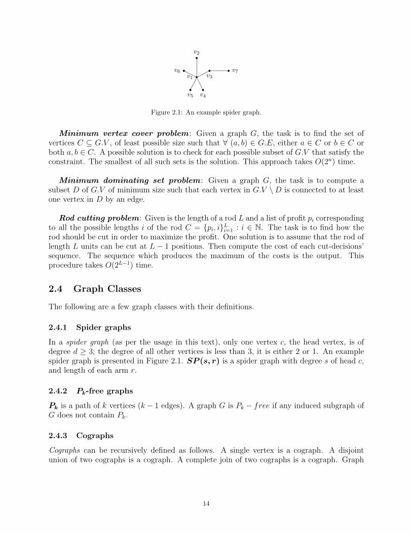
2.4.1 Spider graphs

In a spider graph (as per the usage in this text), only one vertex c, the head vertex, is ofdegree d ≥ 3; the degree of all other vertices is less than 3, it is either 2 or 1. An examplespider graph is presented in Figure 2.1. SP (s, r) is a spider graph with degree s of head c,and length of each arm r.

2.4.2 Pk-free graphs

Pk is a path of k vertices (k − 1 edges). A graph G is Pk − free if any induced subgraph ofG does not contain Pk.

2.4.3 Cographs

Cographs can be recursively defined as follows. A single vertex is a cograph. A disjointunion of two cographs is a cograph. A complete join of two cographs is a cograph. Graph

14

v

(a)

v1 v2

(b)

v1 v2

v3v4

(c)

v1 v2

v3v4

v5

v6

(d)

v1v2

v3v4

v5

v6

(e)

Figure 2.2: a: a single vertex is a cograph; b: a disjoint union of two copies of the cograph in (a) is a cograph;c: a complete join of two copies of the cograph in (b) is a cograph; d: a disjoint union of the cographs in (b)and (c) is a cograph; e: the graph complement of the cograph in (d) is a cograph.

complement of a cograph is a cograph, which is why, cographs are also called complement-reducible graphs. Cographs are P4-free graphs. A few examples of (recursively) con-structed cographs are presented in Figure 2.2.

2.4.4 Disk Graphs

A graph G is a disk graph if there is an edge between a pair of vertices iff the circles drawn onthe plane with those vertices as centers overlap. These circles can generally be of arbitraryradius. If radius of all the circles overlap, the graph is called a unit disk graph .

For example, let a circle C of radius R = 2 be positioned on the plane at (0, 0), three moredisks c1, c2 and c3, each of radius r = 1, is placed with their centres respectively at (2, 0),(0, 2), and (−2, 0). Let us assume that a chain of 4 disks Ch1 = (c11, c

21, c

31, c

41) is attached to

c1 such that c11 overlaps with c1 and c21 only, c41 overlaps with c31 only, and ∀ 2 ≤ j ≤ 3, cj1overlap with only cj−11 and cj+1

1 . Exactly in the similar way, there is a chain behind each ofc2 (Ch2 = (c12, c

22, c

32, c

42)) and c3 (Ch3 = (c13, c

23, c

33, c

43)).

There are q = 3 chains of disks, and p = 4 more disks behind the first disk in each chain.Let Ch = Ch1, Ch2, Ch3 and Cir = c1, c2, c3We denote this network of disks by DK(R,r, q, p, C, Cir, Ch) = DK(2, 1, 3, 4, C, Cir, Ch).

Let the vertex corresponding to C be called head h, vertices corresponding to ci be calledvi, and the vertices corresponding to cji be called vji , ∀ 1 ≤ i ≤ 3, and ∀ 1 ≤ j ≤ 4. Thegraph formed by this setting will be a spider graph SP (3, 5), as shown in Figure 2.3.

Another example of an arrangement of disks is shown in Figure 2.4.

2.4.5 Interval Graphs

An interval graph is formed from a set of intervals on the real line where each intervalis represented as a vertex and there is an edge between two vertices if an only if theircorresponding intervals overlap on the real line.

Interval graphs from a set of intervals

The input is the list of intervals L, each interval i has a starting time si and an ending timeei. Each interval in L corresponds to a vertex in G.

To convert a set of intervals to an interval graph, for each interval a ∈ L, a vertex vais added to G.V . Wherever there is an overlap between any two distinct intervals a and b,a, b ∈ L, that is, if sb ≥ sa and sb < ea, we add an edge (va, vb) in G.E. After following

15

C c1 c11 c21 c31 c41

c2

c12

c22

c32

c42

c3c13c23c33c43

(a)

h

v1

v2

v3

v11

v12

v13

v21

v22

v23

v31

v32

v33

v41

v42

v43

(b)

Figure 2.3: (a) arrangement of disks and (b) the corresponding disk graph, geometrically not according tothe arrangement of the disks, but connections according to the overlap of respective disks.

C ′

c1

c2

cq

Figure 2.4: Central disk C ′ and a set of Cir = c1, c2, ..., cq disks with their circumference touching thecircumference of C ′, and not overlaping with each other, or with C ′

16

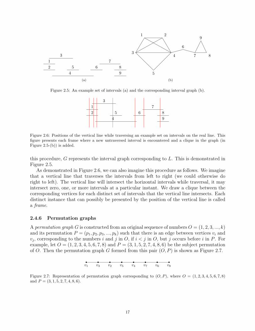
1

2

3

4

5 6

7

8

9

(a)

1 2

34

5

6

7 8

9

(b)

Figure 2.5: An example set of intervals (a) and the corresponding interval graph (b).

1

2

3

4

5 6

7

8

9

Figure 2.6: Positions of the vertical line while traversing an example set on intervals on the real line. Thisfigure presents each frame where a new untraversed interval is encountered and a clique in the graph (inFigure 2.5-(b)) is added.

this procedure, G represents the interval graph corresponding to L. This is demonstrated inFigure 2.5.

As demonstrated in Figure 2.6, we can also imagine this procedure as follows. We imaginethat a vertical line that traverses the intervals from left to right (we could otherwise doright to left). The vertical line will intersect the horizontal intervals while traversal, it mayintersect zero, one, or more intervals at a particular instant. We draw a clique between thecorresponding vertices for each distinct set of intervals that the vertical line intersects. Eachdistinct instance that can possibly be presented by the position of the vertical line is calleda frame.

2.4.6 Permutation graphs

A permutation graph G is constructed from an original sequence of numbersO = (1, 2, 3, ..., k)and its permutation P = (p1, p2, p3, ..., pk) such that there is an edge between vertices vi andvj, corresponding to the numbers i and j in O, if i < j in O, but j occurs before i in P . Forexample, let O = (1, 2, 3, 4, 5, 6, 7, 8) and P = (3, 1, 5, 2, 7, 4, 8, 6) be the subject permutationof O. Then the permutation graph G formed from this pair (O,P ) is shown as Figure 2.7.

v1 v3 v2 v5 v4 v7 v6 v8

Figure 2.7: Representation of permutation graph corresponding to (O,P ), where O = (1, 2, 3, 4, 5, 6, 7, 8)and P = (3, 1, 5, 2, 7, 4, 8, 6).

17

v1

v2v3

v4 v5

v6

v7

v8

v9

v10

Figure 2.8: An example split graph. C = v1, v2, . . . , v5 is the clique and I = v6, v7, . . . , v10 is theindependent set excerpt of this split graph.

2.4.7 Split graphs

A graph G is a split graph if its vertices can be partitioned into a clique and an independentset. A split graph is P5 free. An example split graph is presented in Figure 2.8

18

Chapter 3

Literature Survey

3.1 Graph burning

The burning number was introduced in [10]. This work showed that the burning numberof a path or cycle of length n is d

√ne. They have presented some other properties and

results also related to the graph burning problem. Bessy et al. [7] showed that generalgraph burning is NP-Complete. They showed that optimal burning spider graphs, trees,and path-forests is NP-Complete. A 3-approximation algorithm for burning general graphswas described in [7]. Bonato et al. [11] proposed a 2-approximation algorithm for burningtrees. A 2-approximation algorithm for graphs bounded by a diameter of constant length wasdescribed in [33, 34]. A 1.5 approximation algorithm for burning path forests was describedin [12]. This article also showed that burning number of spider graphs of order n is atmost√n. Simon et al. [1] presented systems that utilize burning in the spread of an alarm

through a network. Bessy et al. [8] proved that the burning number of a connected graph

of order n is at most√

12n7

+ 3 ≈ 1.309√n+ 3. They also showed that the burning number

of trees with n2 vertices of degree 2, and n(≥ 3) vertices of degree at least 3 is at most√(n+ n2) + 1

4+ 1

2. [53] have provided heuristics to minimize the time steps in burning a

graph. They have studied that which vertices should be selected to be burnt from “outside”and in which time-steps.

3.2 Cographs

A cotree [18], constructed from a cograph, assists in the computation of properties of acograph in linear time, such as maximum independent set, graph coloring number, and de-termining if there exists a Hamiltonian cycle. A cograph can be recognized in linear time,and cotrees can be constructed using modular decomposition [17], partition refinement [28],LexBFS [13], or split decomposition [26]. An induced subgraph of a cograph is a cographitself [19].

3.3 Disk graphs

Computation of various properties on disk graph is NP-Hard. Clark et al. (1990) [15]showed that finding the chromatic number of disk graph is NP-Complete. They also showed

19

that 3-coloring problem is NP-Complete on unit disk graph, even if their underlying diskrepresentation is given. Although, in contrast, they also gave a polynomial time algorithm tofind maximal cliques in unit disk graph when the geometrical representation of the underlyingdisks is given.

3.4 Interval graphs

There are several linear time algorithms available to solve different problems on intervalgraph. Olariu [48] discovered linear time algorithm for coloring. Marathe et al. [42] gave alinear time algorithm to compute minimum vertex cover. Similarly, a linear time algorithmto compute interval graph isomosphism was given in [40]. Ibarra [32] proposed a linear timealgorithm to compute the clique separator graph of a given interval graph. Fomin et al. [23]described an algorithm which solves the firefighter problem on interval graphs in O(n7) time.Interval graph ordering was introduced in [49]. As per interval graph ordering, the verticesare ordered according to the increasing order of the ending time of their correspondingintervals. Ravi et al. [50] proposed an algorithm to solve all pairs shortest path in (O(n2))time, where n is the number of vertices. Authors in [33, 34], along with [35] discussed boundson the burning number of interval graph. Although they have not provided any algorithmto find an optimal burning sequence.

3.4.1 Similarity between a path and an interval graph

Proposition 3.1. Let l, r ∈ L be two intervals such that PL (shortest path between l and r)is of maximum length as compared to shortest path between any pair of intervals in L. Then,for each interval i ∈ L, if i 6∈ PL, then i shall overlap with at least one interval of PL.

Proof. Let s = min sj : j ∈ PL and e = max ej : j ∈ PL. Let that i does not overlap withany interval in L, then either (1) ei < s, or (2) si > e.

First let ei < s for contradiction. Let P ′L be the shortest path between i and l, and P ′′L bethe shortest path between i and r. Here, we obtain a contradiction because P ′′L ≥ PL+P ′L−1and P ′ ≥ 2 |P ′′L|, so PL is not of maximum length. Otherwise, L may be disconnected.

Similarly, we can obtain a contradiction for an interval i such that si > er.

Corollary 3.1. Let P be the shortest path between a pair of vertices in G, which is ofmaximum length as compared to the shortest path between any other pair of vertices in G.V ,that is, P is the diameter of G, then all vertices in G \P are connected by a single edge withat least one of the vertices in P .

Corollary 3.1 has been proved earlier in [35] and [33, 34]. It can also be observed thatthe interval graphs do not contain a cycle of size more than 3 [25, 27]; we show this inProposition 3.2.

Proposition 3.2. For any induced subgraph G′ of an interval graph G with |G′.V | 6= 3, G′

will not be a cycle.

Proof. Let the interval graph be a cycle of k ≥ 4 vertices v1, v2, v3, ..., vk corresponding to theintervals i1, i2, i3, ..., ik respectively. The interval ij overlaps with interval ij+1, ∀1 ≤ j ≤ k−1.Now to validate this cycle, interval i1 must overlap with ik. This is only possible if either orboth of the following occur.

20

i1

i2

ik−1

ik

Set of intervals

(a)

v1 v2

vk−1 vk

Corresponding interval graph

(b)

Figure 3.1: Demonstration of what happens if we try to create an interval graph cycle and the correspondingset of intervals. The dotted lines are the prospective edges which shall form, apart from the original cycle ofk vertices. Either or both of the terminal vertices v1 or vk, on the original path v1, ..., vk shall be connectedto all the vertices from v2, v3, . . . , vk−1.

(a) i1 overlaps with all intervals i2, i3, i4, ..., ik−1 also.(b) ik overlaps with all intervals i2, i3, i4, ..., ik−1 also.

Here we obtain the contradiction that there will not exist cycle of length greater than 3 inany induced subgraph of G. This is demonstrated in Figure 3.1.

Corollary 3.2. We can conclude two simple facts, which are as follows.(1) If a vertex v of G is not in P , then it is adjacent to some vertex in P , it is part of a

clique involving that vertex of P .(2) Each clique involves exactly

(a) one vertex from P or(b) two vertices from P which are adjacent according to the sequence of P .

3.5 Permutation graphs

Polynomial time algorithms exist for various properties in permutation graphs. If r is thesize of longest decreasing subsequence in a permutation P , then the chromatic number andthe size of largest clique in the corresponding permutation graph G, both are equal to r [27].Atallah et al. (1998) [3] proposed an algorithm that finds the minimum dominating set inan arbitrary permutation graph with n vertices in O(n log2 n) time.

3.6 Split graphs

Clearly, it is easy to compute the maximum clique on split graphs, and complementarily, itsmaximum independent set [27, 29]; along with coloring. [35] showed that split graphs can beburned in polynomial time. Determining if a hamiltonian cycle exists remains NP-Completefor split graphs [47], along with the minimum dominating set problem [6].

21

Chapter 4

Graph burning: Problem statement

4.1 Introduction

Works like [5, 21, 36, 37, 46, 51] have studied the spread of social influence in order to analyzea social network. [39] have highlighted that the underlying network plays an essential role inthe spread of an emotional contagion; they have nullified the necessity of in-person interactionand non-verbal cues.

With the aim to being able to model such problems, graph burning was introduced in [10].Graph burning runs on discrete time-steps. During a graph burning process, each vertex iseither burned or unburned. We choose one unburned vertex in each step as a “fire source”.If a node is burned, then it remains in that state until the end of the game. Once a node isburned in time-step t, it spreads fire to its neighbouring vertices in step t+ 1 and each of itsunburned neighbours are also burned. The aim of the graph burning problem is to burn allthe vertices in a given graph G in least amount of time-steps. Formally, we describe graphburning as follows.Arbitrary graph burning: At each step t, first (a) an unburned vertex is burned (as afire source) from “outside”, and then (b) the fire spreads to vertices adjacent to the verticeswhich are burned till step t − 1. This process stops after all the vertices of G have beenburned.

Burning process on an example graph has been demonstrated in Figure 4.1. Observe thatthere are 4 fire sources that burn this graph in this particular procedure. We define burningsequence of an arbitrary graph G in Definition 4.1 as follows.

Definition 4.1. Burning sequence. The burning sequence of a graph G is the sequence ofvertices that were chosen as fire sources in part (a) of each time-step to burn a given graph,such that this sequence of vertices is able to burn all the vertices of G.

In the graph demonstrated in Figure 4.1, the burning sequence is S = (r, q, s, w). Thismeans that r was chosen as a fire source in step 1a, q was chosen as a fire source in step 2a,and so on.

4.2 The underlying problem

Graph burning aims to burn all the vertices in a graph as quickly as possible and hasbeen inspired by other contact processes like firefighting [30], graph cleaning [2], and graph

22

p q

r st

uv

w

(a)

p q

1ar st

uv

w

(b)

p 2a q

1ar st

uv

w

(c)

2bp 2a q

1ar st

uv

w

(d)

2bp 2a q

1ar 3ast

uv

w

(e)

2bp 2a q

1ar 3as3b t

uv

w

(f)

2bp 2a q

1ar 3as3b t

uv

4a w

(g)

2bp 2a q

1ar 3as3b t

4bu4b v

4a w

(h)

Figure 4.1: Burning a graph. See that part b does not run in step 1 because there is no vertex that wasburnt before step 1, so the fire did not spread. Once we label the vertex in some step, we do not change thelabel in any future steps.

bootstrap percolation [4]. The underlying decision problem is described as follows.The decision problem: Given input is an arbitrary graph G and a constant k. The

problem is to determine if G can be burnt using a burning sequence of length k or less (orequivalently, in k or less time-steps).

Equivalently, we have the optimization version of the graph burning problem.The optimization problem: Given input is an arbitrary graph G. The problem is

to compute the minimum number of fire sources (or equivalently, time-steps), that can(collectively in the form of a burning sequence) burn G completely.

With reference to the theory that we established in Chapter 1, it can be observed thatif an optimization algorithm returns a positive integer k as output, the decision algorithmwill return true if the input (G, k) is passed to it. Note that the main task in the burningproblem is to find a burning sequence of minimum length such that it is able to to burn allthe vertices of a graph. Here, we introduce a (new) property of a graph G in Definition 4.2,the burning number of a graph G [10], which we denote as b(G).

Definition 4.2. Burning number. The least amount of time steps (or equivalently, firesources) which are required to burn a graph G is called the burning number of G, b(G).

Clearly, the burning number of a graph G tells that how fast G “can” be burnt. Observefrom Figure 4.2 that the same graph that we burnt in four time-steps in Figure 4.1, canalso be burnt in only three time-steps. From Figure 4.2, we have that the burning sequenceS ′ = (q, v, u) of size 3 is also able to burn this graph completely.

Observe that the example graph, on which two different burning procedures are demon-strated, in Figure 4.1 and Figure 4.2 respectively, requires at least 3 time steps to be burnt;

23

p q

r s

t

u

v

w

(a)

p 1a q

r s

t

u

v

w

(b)

p 1a q

r s

t

u

2a v

w

(c)

2bp 1a q

2br 2bs

2b t

u

2a v

w

(d)

2bp 1a q

2br 2bs

2b t

3au

2a v

w

(e)

2bp 1a q

2br 2bs

2b t

3au

2a v

3b w

(f)

Figure 4.2: (Better) Burning procedure (optimal) on an example graph. The subject graph is same as thaton which an arbitrary burning procedure is demonstrated in Figure 4.1.

it cannot be burned in less than 3 time steps. So S ′ is an optimal burning sequence whichcan burn this graph. Burning number of this graph is 3.

Let that a burning procedure burns a graph in k time steps. While burning a graph,it is noticeable that if at a step i a vertex v ∈ G is chosen as a fire source, then at eachsubsequent step, the set of vertices to which v spreads fire to keeps on increasing till the kth

step: at a time step i + t, v is able to burn all the vertices in G.Nt[v]. Here, we define theburning cluster of a fire source in Definition 4.3 as follows.

Definition 4.3. Burning cluster. Let that a burning sequence S = (x1, x2, . . . , xk) of sizek is able to burn a graph G. The burning cluster of a fire source xi (the fire source chosenat the time-step i) is the set of vertices to which xi is able to spread fire till the end of theburning process (till the kth time-step). This set contains all the vertices in G.Nk−i[xi].

If S = (x1, x2, x3, ..., xk) is the burning sequence which is capable of burning G, Equa-tion (4.1) [7] must follow.

G.Nk−1[x1] ∪G.Nk−2[x2] ∪ ... ∪G.N0[xk] = G.V. (4.1)

Some results that have been discovered with respect to graph burning are present inSection 3.1.

24

4.3 Verification of a burning sequence

As discussed in Section 1.6, a problem which can be verified deterministically in polynomialtime is in NP class. We can verify the validity of a burning sequence in polynomial time.Every burning sequence which satisfies Equation (4.1) is is able to burn G completely, butapart from this, here we also verify that no fire source in a burning sequence should beplaced on the vertex which has already been burnt. Algorithm 4.1 verifies if a given burningsequence S is a valid burning sequence for a graph G.

Algorithm 4.1. Given an input graph G and a burning sequence S = (x1, x2, x3, ..., xk) oflength k, perform the following steps.

Stage 1. If S does not satisfy Equation (4.1), then return false.Stage 2. ∀ 1 ≤ i ≤ k − 1, perform the following steps.Stage 2.1. ∀ i+ 1 ≤ j ≤ k, if xj ∈ G.Nj−i−1[xi], then return false.Stage 3. Return true.

If Algorithm 4.1 returns true for the input (G,S), it means that S is a valid burningsequence and is able to burn G completely. Algorithm 4.1 can be implemented in O(n2)time. This also implies that the graph burning problem is in NP. We state the formally inLemma 4.1. In fact, optimal burning of general graphs is NP-Hard. We discuss this in thefollowing chapters in detail.

Lemma 4.1. The (optimal) graph burning problem is in NP.

4.4 Related problems and games

As discussed in Section 4.2, the procedures of certain other problems such as firefighterproblem, graph cleaning and graph bootstrap percolation are similar to the procedure of thegraph burning problem. In the following few paragraphs in this section, we shall discussthem in brief.

4.4.1 Firefighter problem

The aim of the firefighter problem [23] is to save as many vertices of a given graph G aspossible from a fire that starts from a single vertex. At step 1, an arbitrary vertex is burned.At each step t, t ≥ 2, first (a) a firefighter can be placed on an unburned vertex and thisfirefighter protects that node from fire till the last time-step, and then (b) the fire spreadsto the unprotected vertices adjacent to the vertices which are burned till step t − 1. Thisprocess continues till fire cannot spread to any more vertices.

The input is the subject graph G and one fire source s. The task is to save the maximumpossible number of vertices from fire.

4.4.2 Firefighter reserve problem

Firefighter reserve deployment [23] problem proceeds as follows. The fire gets initiated froma single fire source. Initially, there is one firefighter in the firefighter reserve. In each stept, t ≥ 2, (a) some or no firefighters (subject to availability in the firefighter reserve) are

25

placed, each on an unburned vertex, (b) the fire spreads from the burned vertices to theiradjacent vertices which are not protected (by a firefighter), (c) one firefighter increases inthe firefighter reserve. This process continues until fire can spread no further.

4.4.3 Graph cleaning

In the graph cleaning problem, at the beginning, all the vertices and the edges are considered“dirty”. There are a fixed number of available cleaning brushes. At each step, one vertex vand all the edges incident to v which are dirty may be cleaned if the number of brushes on vare equal to the dirty edges incident on v. No brush cleans any edge which is already clean.If a brush cleans an edge, the edge is considered to be traversed. A vertex is cleaned if allthe edges incident to it are cleaned, and the cleaning process is done on a vertex v only ifwe can clean each edge incident on it. A graph G is considered cleaned when each vertex ofG has been cleaned. Graph cleaning was introduced in [43, 45].

The input is an arbitrary graph G, and a constant k number of brushes. The task is todetermine if G can be cleaned by k brushes. Equivalently, the optimization problem can beto compute the minimum number of brushes that are required to clean an arbitrary graph.

4.4.4 Graph bootstrap percolation

A phenomenon in graphs called weak saturation was introduced by Bollobas in 1968. Givena graph H, another graph G of n vertices is called weakly H-saturated if no subgraph of Gcan make H, but ∃ a non-empty set A consisting of edges missing in G such that ∀ e ∈ A,H is a subgraph of G+ e [22, 4, 9]. [4] observed that weak saturation is strongly related tobootstrap percolation, which was introduced in [14].

In bootstrap percolation, the inputs are an arbitrary graph G and an infection thresholdr > 2. We choose a set of initially “infected” vertices A ⊆ G.V ; we declare the remainingvertices G.V \ A “healthy”.

Then, in consecutive time steps, we infect all healthy vertices which have at least r infectedneighbours. We say that A percolates if, starting from A we are able to finally infect everyvertex in G.V . More precisely, we set A0 = A and for t = 1, 2, 3, ..., we compute At accordingto Equation (4.2) [22] as follows.

At = At−1 ∪ v ∈ V : |G.N [v] ∩ At−1| ≥ r (4.2)

Hence A percolates if after computing on equation 0.2 indefinitely, we infect all the ver-tices, that is, ∪∞t=0At = G.V .

4.5 Overview of possible applications

Burning a graph can be used to model the spread of a meme, social gossip, emotion, or asocial contagion. It can also be used to model spread of viral infections, or otherwise theexposure to infections and proliferation of virus in the body. Graph burning is relatively anewly introduced procedure. Currently, not much works have come in public domain whichutilize the graph burning in modelling of practically applicable systems.

Simon et al. [1] have provided heuristics for usage in for spreading an alarm or other crit-ical information in minimum amount of time steps. This may include spread of information

26

via satellite, or throughout a terrestrial network, for example. They have assumed that asatellite can spread information only sequentially: to one target node (person, device, etc)at a time. On the other hand, each node in their system is able to spread the informationparallelly through the available technologies.

Simon et al. [53] have simulated a network which tries to spread alarms to all the nodesin the least amount of time steps. The nodes are connected to each other, and at the startof each time step, a new node is alarmed from “outside”. Also during each time step, thealarmed nodes alarm their neighbour nodes, same as the graph burning procedure. Thisprocess stops when all the nodes are alarmed.

4.6 Computational limitations

Optimal graph burning is hard [7] for general graphs, like several other problems such ascoloring a graph, finding the largest clique in a graph, or finding maximum sized independentset of a graph. It has been shown that graph burning is NP-Complete for several graphclasses, even when computing other properties, which are NP-Hard for general graph classes,is “easy”: graph classes on which other NP-Hard problems can be solved in polynomial time.It has been proved in [7] that burning a spider graph, path forests, and trees with maximumdegree 3 is NP-Complete.

On the other hand, we have a 3-approximation algorithm for burning general graphs, a2-approximation algorithm for burning trees, a 2-approximation algorithm for burning thegraphs bounded by a diameter of constant length, and a 1.5-approximation algorithm forburning path forests, as discussed in Section 3.1.

In the following chapters, we discuss these characteristics of the graph burning problemin detail from the perspective of certain graph classes. For the overview of chapters, seeSection 1.11.

4.7 Summary of this chapter

Graph burning represents the multiplication and spread of an object or phenomenon through-out a network under some strict constraints. One of the important aspect is, in each time-step, an object/phenomenon infects one of the uninfected nodes. Despite of its high compu-tational complexity, it can be further utilized to model some useful processes in a computer.

27

Chapter 5

The burning process in graphs

5.1 Burning a simple path or cycle

A path is simple to burn. A path and a cycle (of equal length) are equivalent from theburning perspective. In each step, we select one new unburnt “victim” vertex (a fire source)and burn vertices adjacent to other clusters. This follows from the definition of graph burningthat we discussed in Section 4.1. Each cluster burns its neighbour vertices and includes themin itself. The interesting fact here is, a burning cluster can spread fire to atmost two morevertices. Each burning cluster starts with on single vertex (a fire source) and in successivetime steps, it can get enlarged in size by atmost two more vertices. A newly burned firesource also acts as a distinct cluster.

5.1.1 Burning a path (or a cycle) of infinite length

Let us consider that a path is so long (of infinite length) that we can put fire sources insuch a way that any two fire sources are at infinite distance from one another, as shownin Figure 5.1. We select a fire source, and the fire in all other clusters spreads to theirrespective neighbouring vertices, i.e., each burning cluster has 2 more vertices; this is shownin Table 5.1.

For a burning cluster, initially it is born with a single vertex, and 2 more vertices keepon adding to it in all the subsequent steps.

C1 C2 C3 C4 C5 • • •Step 1 1Step 2 2 1Step 3 2 2 1Step 4 2 2 2 1Step 5 2 2 2 2 1

•••

Total 25 9 7 5 3 1 • • •

Table 5.1: Step-wise number of burned vertices in all the clusters Ci in a path of infinite length, as shownin figure 1. Total burning vertices shown at bottom left.

28

original path (step 0)

(a)

1a

(b)

1a

2a

(c)

1a

2a

3a

(d)

1a

2a

3a

4a

(e)

and so on

Figure 5.1: Burning process on a path of ∞ length; the fire sources are placed at ∞ distance from eachother.

29

Step 3 3b 2b 1a 2b 3b 3b 2a 3b 3a

Step 2 2b 1a 2b 2a

Step 1 1a

Step 0

Figure 5.2: Burning of a path of 9 vertices (optimal procedure). The vertices are marked by the step numberin which they are burned. For each step, the vertex which is selected (arbitrarily) as a victim to be burned(the fire source) is marked by a , and those which are burned by the fire spread from already burned verticesare marked by b.

5.1.2 Governing dynamics

Equation (5.1) and Equation (5.2) show the phenomenon of initiating one fire source at astep t along with the addition of two more vertices to the clusters created in the previoussteps.

f0 = 0 (5.1)

ft = ft−1 + 1 + 2(t− 1) = 2t− 1 + ft−1 (5.2)

For a path of finite length, in each step, we must burn an unburnt vertex such that theburning clusters do not coincide uptil the maximum number of possible time steps. ft inEquation (5.2) presents the maximum of vertices that can be burnt in a given path untilafter the completion of step t.

Equation (5.1) and Equation (5.2) imply that ft is the sum of first t odd numbers, whichis equal to t2; ft = 1 + 3 + 5 + ...+ (2t− 1) = t2. So we have that a path of length n shouldtake at least

⌈√n⌉

time steps to burn completely. While burning a path of finite length,

after step t we shall have burnt atmost t2 vertices. [10] have shown that it takes⌈√

n⌉

stepsto burn a path of n vertices. They also gave an algorithm to compute an optimal burningsequence for a path of finite length, which we describe as Algorithm 5.1.

Algorithm 5.1. Given the input (G, P ) where G is the graph denoting a path, P is asequence of vertices in the path represented by G from (any) one end to the other, and P [i]stands for ith vertex in P , perform the following steps.

Stage 1. n = |P |. S = φ. k =⌈√

n⌉.

Stage 2. ∀ 0 ≤ i ≤ k − 2, v = n− i2 − i; S = S ∪\s P [v].Stage 3. If n > (k − 1)2 + k, then v = n− (k − 1)2 − (k − 1);

else, then v = 1.S = S ∪\s P [v].

Stage 4. Return S.

Time complexity of Algorithm 5.1 is O(√n), where n is the number of vertices in a given

path.The optimal burning process of a path of 9 vertices is demonstrated in Figure 5.2; the

burning number of this path is 3.

30

5.2 Optimal burning of some general graphs

We start with defining isometric subgraph. An isometric subgraph of a graph is defined asfollows.

Isometric subgraph: A subgraph H of a graph G is called an isometric subgraph if forevery pair of nodes u and v in H, we have that the shortest distance between them in H isequal to the shortest distance between them in G. If G is a tree, and then we have that His an isometric tree of G is the same conditions satisfy.

It can be easily observed that any connected subgraph of a tree is its isometric subtree.Bonato et al. [10] have showed that if the burning number of a graph G is b(G) = k′, thenthe burning number of H, an isometric subtree of G is b(H) ≤ b(G) = k′. We show this inTheorem 5.1.

Theorem 5.1. Let that the burning number of a graph G is b(G) = k′, then the burningnumber of H, an isometric subtree of G is b(H) ≤ b(G) = k′.

Proof. Let for contradiction that b(G) < b(H). Let the burning number of H be k′. From ourassumption, we have that b(G) ≤ k′ − 1. This implies that there exists a burning sequenceS ′ = (y1, y2, ..., yk′−1) which is able to burn G completely.H cannot be burned by any burning sequence of length less than k′. It means that for any

burning sequence of length less than k′, at least one vertex in H remains unburned. SinceH is an isometric subtree of G, we have that for any burning sequence of length less thank′, at least one vertex in G also remains unburned. So we need at least one more fire sourcein S ′ to burn G which is a contradiction to our assumption.

Similarly, we can obtain a proof that for any graph G, the burning number of an isometricsubgraph of G is not more then its own burning number b(G). Theorem 5.2 and Theorem 5.3we proved in [10].

Theorem 5.2. If a connected graph G is of radius r, then b(G) ≤ r + 1.

Proof. Let v be the vertex from which the distance of each vertex in G.V is atmost r. Letthat we have put a fire source on v in the first time step. ∵ G.Nr[v] = G.V , G will eventuallyget burnt within r more time-steps irrespective of the position of the fire sources that areput in all other time-steps.

Theorem 5.3. Let that G is a graph containing k connected components, each having aradius atmost r, then b(G) ≤ r + k.

Proof. Let there be k components C1, C2, . . . , Ck in a graph G, each of maximum radius r.Let vi be a vertex in Ci, ∀ 1 ≤ i ≤ k, such that it is atmost at a distance r from all the othervertices in Ci.

Let that in each time-step we put a fire source such that in step i, we put a fire sourceon vi. Within next r time-steps G will be burnt.

Next we discuss the burning procedure on some examples of spider graphs. SP (3, 4) canbe burnt optimally in 4 steps. As demonstrated in Figure 5.3, an optimal burning sequenceof the presented graph SP (3, 4) is S ′SP (3,4) = (b, h, l, m), which is of size 4.

If we increase one more arm in SP (3, 4), it becomes SP (4, 4), and now we need at least5 time steps to burn it; a burnt SP (4, 4) is shown in figure Figure 5.4. An optimal burningsequence of the presented graph SP (4, 4) is S ′SP (4,4) = (b, h, l, m, q).

31

a

b c d e

f g h i

j k l m

(a)

a

1a

bc d e

f g h i

j k l m

(b)

2b

a

1a

b

2b

cd e

f g

2a

hi

j k l m

(c)

2b

a

1a

b

2b

c

3b

de

3b

f

3b

g

2a

h

3b

i

3b

jk

3a

lm

(d)

2b

a

1a

b

2b

c

3b

d

4b

e

3b

f

3b

g

2a

h

3b

i

3b

j

4b

k

3a

l

4a

m

(e)

Figure 5.3: Optimal burning of SP (3, 4).

2b

a 1a

b

2b

c

3b

d

4b

e

3b

f

3b

g

2a

h

3b

i

3b

j

4b

k

3a

l

4a

m

3b

n

4b

o

5b

p

5a

q

Figure 5.4: Optimal burning of SP (4, 4)

32

y1

yk′

y2

y3

y4

Figure 5.5: Optimal burning of a graph SP (d, k′ − 1), where d ≥ k′ + 1. S′SP (d,k′−1) = (y1, y2, ..., yk′) is theoptimal burning sequence.

Bessy et al [7] have proved that for a graph SP (s, r) if s ≥ r, then b(SP (s, r)) = r + 1,and if s ≥ r + 2, then it is necessary for any optimal burning sequence to have first firesource on the spider head. We show this as Lemma 5.1. Figure 5.5 is an example of thisphenomenon; it shows burning of SP (d, k′ − 1), where d ≥ k′ + 1. In its optimal burningsequence S ′SP (d,k′−1) = (y1, y2, y3, ..., yk′), the first fire source y1 is placed on the spider head.

Lemma 5.1. For a graph SP (s, r) if s ≥ r, then b(SP (s, r)) = r + 1, and if s ≥ r + 2,then it is necessary for any optimal burning sequence to have first fire source on the spiderhead.

Proof. We start with discussing a spider graph SP (r, r) whose number of arms r is equalto the length of each arm. The radius of SP (r, r) is r. So by Theorem 5.2 we have thatb(SP (r, r)) ≤ r + 1.

Now we show that b(SP (r, r)) ≥ r + 1. Let for contradiction that b(SP (r, r)) ≤ r. Thisimplies that there is a w-burning sequence S ′ = (x1, x2, ..., xk′) such that k′ ≤ r which isable to burn SP (s, r). No fire source in S ′ shall be able to burn more than one leaf node inG because the distance between any two leaf nodes is 2r. We will be able to burn atmostk′ ≤ r leaf nodes in k′ rounds. This implies that at least 1 leaf node will be left unburned.This implies that S ′ must contain at least one more fire source which is a contradiction.

Thus, b(SP (r, r)) = r + 1.Given that s ≥ r + 2, by Theorem 5.1 b(SP (s, r)) ≥ r + 1. Also since the radius of

SP (s, r) is of radius r, we have that SP (s, r) ≤ r + 1. So we have that SP (s, r) = r + 1.Next we show that if s ≥ r + 2, then it is necessary for any optimal burning sequence

to have first fire source on the spider head. Let that an optimal burning sequence S ′ =(y1, y2, ..., yr+1) of length r + 1 is able to burn SP (s, r). Let for contradiction that the firstfire source is not placed at the spider head. So we have that at least r+1 leaf nodes cannot beburned by y1. Also, no other fire source will be able to burn two leaf nodes simultaneouslybecause the distance between any two leaf nodes is 2r. So we have that the fire sourcesy2, ..., yr+1 will be able to burn at most r leaf nodes. We have that at least one leaf node willremain unburned which is a contradiction. So the first fire source y1 ∈ S ′ must be placed atthe spider head. This concludes the proof.

Figure 5.5 shows burning of a graph containing only one connected component, whereasFigure 5.6 represents the burning of a graph GSP which is a disjoint union of k′ components.

33

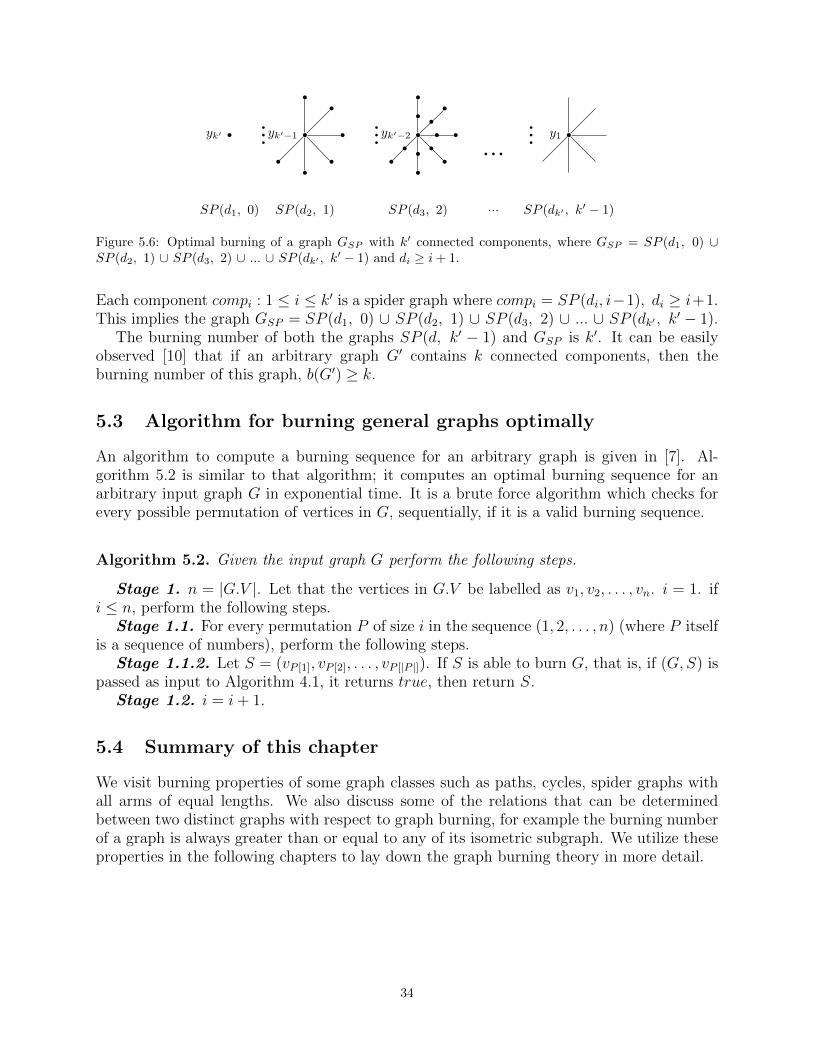
yk′ yk′−1 yk′−2 y1

SP (d1, 0) SP (d2, 1) SP (d3, 2) ... SP (dk′ , k′ − 1)

Figure 5.6: Optimal burning of a graph GSP with k′ connected components, where GSP = SP (d1, 0) ∪SP (d2, 1) ∪ SP (d3, 2) ∪ ... ∪ SP (dk′ , k′ − 1) and di ≥ i + 1.

Each component compi : 1 ≤ i ≤ k′ is a spider graph where compi = SP (di, i−1), di ≥ i+1.This implies the graph GSP = SP (d1, 0) ∪ SP (d2, 1) ∪ SP (d3, 2) ∪ ... ∪ SP (dk′ , k

′ − 1).The burning number of both the graphs SP (d, k′ − 1) and GSP is k′. It can be easily

observed [10] that if an arbitrary graph G′ contains k connected components, then theburning number of this graph, b(G′) ≥ k.

5.3 Algorithm for burning general graphs optimally

An algorithm to compute a burning sequence for an arbitrary graph is given in [7]. Al-gorithm 5.2 is similar to that algorithm; it computes an optimal burning sequence for anarbitrary input graph G in exponential time. It is a brute force algorithm which checks forevery possible permutation of vertices in G, sequentially, if it is a valid burning sequence.

Algorithm 5.2. Given the input graph G perform the following steps.

Stage 1. n = |G.V |. Let that the vertices in G.V be labelled as v1, v2, . . . , vn. i = 1. ifi ≤ n, perform the following steps.

Stage 1.1. For every permutation P of size i in the sequence (1, 2, . . . , n) (where P itselfis a sequence of numbers), perform the following steps.

Stage 1.1.2. Let S = (vP [1], vP [2], . . . , vP [|P |]). If S is able to burn G, that is, if (G,S) ispassed as input to Algorithm 4.1, it returns true, then return S.

Stage 1.2. i = i+ 1.

5.4 Summary of this chapter

We visit burning properties of some graph classes such as paths, cycles, spider graphs withall arms of equal lengths. We also discuss some of the relations that can be determinedbetween two distinct graphs with respect to graph burning, for example the burning numberof a graph is always greater than or equal to any of its isometric subgraph. We utilize theseproperties in the following chapters to lay down the graph burning theory in more detail.

34

Chapter 6

Other games and problems

In this chapter, we are going to describe some problems which are related to the graphburning problem, and some problems which we utilize in the following chapters to provevarious properties of graph burning.

6.1 Distinct 3-partition problem

For definition of the distinct 3-partition problem, see Section 2.3. [31] have showed that thedistinct 3-partition problem is NP-Complete in the strong sense. So as per our discussion inSection 1.7, we have that if each element of the input set is bounded above by the polynomialin the length of the input, then the distict 3-partition problem still remains NP-Complete.

We have from Lemma 1.1 and lemma 1.2 in Section 1.8 that if a problem B (which isNP-Complete in the strong sense) is reducible (in polynomial or pseudo-polynomial time)to another problem B′ which is in NP, we have that B′ is also an NP-Complete problem inthe strong sense. We reduce several problems from the distinct 3-partition problem in thefollowing chapters to show the NP-Completeness of various graph burning subproblems (inthe strong sense).

6.2 Firefighter problem

The firefighting game, in combination with graph burning, can be used to model, for exam-ple, various “real-life” social scenarios where (communicable) diseases are spread. We alsodiscuss (briefly) majorly in the conclusion how the firefighting game can be used to modelthe hindrance to the spread of a disease (the spread of which, we can model through graphburning). In fact, firefighter was introduced (in [30]) to capture several important applica-tions which included immunization of a population against a virus. In this section, we brieflydiscuss the firefighter problem. For the definition of the firefighter problem, see Section 4.4.

In the firefighter problem, we input an arbitrary graph G, and a vertex s ∈ G.V which isthe initial fire source. After the computation of a firefighting process, a sequence of verticesS is generated which is used, (sequentially) one vertex in each round, to put the firefighteron, and thus, protect it the spread of fire. Once a vertex is protected, it cannot be burnt(and so it can also not spread the fire). Lemma 6.1 was proved in [23].

35

Lemma 6.1. We can verify the solution for a firefighter problem on a graph G of n verticesand m edges with a fire source s in O(n+m) time. [23]

Proof. The input is G, s, and a sequence S of vertices where the firefighter is placed inthe (same) sequence of time steps. The vertices on which firefighter is placed till step i isSi = S[1 : i− 1], an algorithm is described as Lemma 6.1.

Algorithm 6.1. Given the input (G, s, S), perform the following steps.

Stage 1. B = s (stores the set of vertices which have been burnt). k = |S|.Stage 2. ∀ 2 ≤ i ≤ k, perform the following steps.Stage 2.1. If S[i] ∈ T , then return false.Stage 2.2. B = B ∪ (G \ S[1 : i− 1]).Adj[B].Stage 3. If B ∪ (G \ S).Adj[B] = B (that is, if fire can spread no more), then return

true, else return false.

Corollary 6.1. The firefighter problem is in NP.

Lemma 6.2. The firefighter and the firefighter reserve deployment problem are the same.[23]

Proof. Followed by the definitions (see definitions of both in Section 4.4).

Lemma 6.3. Given the instance (G, s) of a firefighter problem if l is the number of verticesin a longest induced path in G, starting in s, then no optimal strategy can place firefighteron more than l − 1 vertices. [23]

Proof. Let the firefighter sequence be S = (v1, v2, ..., vt). Let P be a path between vt and ssuch that all vertices in P burn, except vt. Let that P is the only path with this property.=⇒ |P | ≥ t+ 1, or otherwise not have protected vt in tth step. Therefore, t ≤ l − 1.

Theorem 6.1. Firefighter problem can be solved in O(nk−2(n+e)) = O(nk) time for Pk-freegraphs. [23]

Proof. In a Pk-free graph G, the longest induced path is of length k− 1. By Lemma 6.3, anyoptimal strategy protects at most k − 2 vertices.

Proof of Theorem 6.1 suggests the algorithm Algorithm 6.2 as follows, which is able toperform the firefighting problem in a Pk-free graph G in O(nk−2(n + m)) time (where n isthe number of vertices in G and m is the number of edges in it).

Algorithm 6.2. Given an input graph G, perform the following steps.

Stage 1. Enumerate all ordered subsets S ⊆ V (G) of size at most k − 2 in nk−2 time.Stage 2. For each S, perform the following steps.Stage 2.1. Verify by lemma 0.2 that it is a valid firefighter sequence in O(n+m) time.Stage 2.3. If S is a valid firefighter sequence, then return S.

Corollary 6.2 has been proved in [23].

Corollary 6.2. Firefighter problem can be solved on split graphs in polynomial time.[23].

Proof. Since split graphs are P5 free graphs, this corollary follows from Theorem 6.1.

36

6.3 Firefighting general graphs

Algorithm 6.3 computes an optimal firefighting sequence for an arbitrary input graph G inexponential time. It checks for every possible permutation of vertices in G, sequentially, ifit is a valid firefighting sequence. It is a brute force algorithm.

Algorithm 6.3. Given the input (G, s), where G is an arbitrary graph, and s ∈ G.V is theinitial fire source, perform the following steps.

Stage 1. n = |G.V |. Let that the vertices in G.V be labelled as v1, v2, . . . , vn. i = 1.Smax is the firefighting sequence which saves maximum vertices and m is the number ofvertices saved by Smax, initially m = 0, Smax = φ. If i ≤ n, perform the following steps.

Stage 1.1. For every permutation P of size i in the sequence (1, 2, . . . , n) (where P itselfis a sequence of numbers), perform the following steps.

Stage 1.1.2. Let S = (vP [1], vP [2], . . . , vP [|P |]). If S is is a valid firefighting sequence byAlgorithm 6.1 (Lemma 6.1), then if m > the total number of vertices protected and savedby S, then Smax = S and m = the number of vertices protected and saved by S.

Stage 1.2. i = i+ 1.Stage 2. Return Smax.

Using Algorithm 6.3, we compute a valid firefighting sequence which is able to protectand save the maximum number of vertices in G. In-spite of computing this throughout allthe permutations of all sizes in v1, v2, . . . , vn, we could also return the first valid firefightingsequence that we encounter, but that would not suffice the task of saving the maximumvertices.

6.4 Summary of this chapter

We discuss the distinct 3-partition problem, which we are going to reduce to the burningseveral graph classes to show that the problem is NP-Complete for these graph classes. Wealso discuss the firefighter problem which we can utilize to use with graph burning to modelprotection of a graph against graph burning. We discuss some of the models that can bebuilt using this concept towards the conclusion, Chapter 10.

37

Chapter 7

Why is burning hard?

In this chapter, we describe some of our novel results in Section 7.1, Section 7.2, and Sec-tion 7.3. Respectively, we show that burning interval graphs, permutation graphs and diskgraphs is NP-Complete. In fact, NP-Completeness of burning disk graphs follows from theNP-Completeness of interval graphs, but our construction in the proof for disk graphs issuch that another class of graphs follows to be NP-Complete from it.

As corollaries of our results in these sections, it follows that burning several other graphclasses remains NP-Complete. These corollaries are obtained for those graph classes for whichNP-Completeness results have been shown earlier. We provide citations to the resourceswhere the respective results were first discussed.

7.1 Burning interval graphs

7.1.1 Similarity in burning paths and interval graphs

Refer to the definition of the burning cluster of a fire source, described as Definition 4.3 inSection 4.2. While demonstrating the burning of a path or cycle in Section 5.1, we obtainan observation described as Observation 7.1 as follows.

Observation 7.1. The burning clusters of each of the n fire sources of any optimal burningsequence of a path of order n2 are pairwise disjoint.

From Corollary 3.1 in Section 2.4.5, Observation 7.2 follows, which we describe as follows.

Observation 7.2. Let P be a shortest path of maximum length among shortest paths betweenall pairs of vertices in an interval graph G. Then b(P ) ≤ b(G) ≤ b(P ) + 1.

Observation 7.2 has been shown earlier in [35, 33, 34].Finding such P is easy to do in polynomial time. We can simply compute all pair shortest

path and choose the maximum length path among all. So burning an interval graph in(b(P ) + 1) is trivial. We study if b(G) = b(P ), whether it is always possible to determine thesame and compute a burning sequence of length b(P ). We show that this is an NP-Completeproblem. We use the distinct 3-partition problem (see Section 6.1) and reduce it to intervalgraph burning to show NP-Completeness of this graph burning subproblem.

38

u1j

x1

vt

v vr x2

u|Tj |−2j

Figure 7.1: Structure of a Tj with 33 vertices, along with the extra vertices connected to it. The dashed linerepresents the fact that other subpaths may be connected to a Tj on either or both ends.

7.1.2 Interval graph construction for NP-completeness

Let X be an input set to the distinct 3-partition problem; let n = |X|3

, m = max(X),

B = s(X)n

, and k = m−3n. Let Fm be the set of firstm natural numbers, Fm = 1, 2, 3, ...,m;and F ′m be the set of first m odd numbers, F ′m = 2 fi − 1 : fi ∈ Fm = 1, 3, 5, ..., 2m− 1.Let X ′ = 2 ai − 1 : ai ∈ X, B′ = s(X′)

n. Observe that s(X ′) =

∑3ni=1 2 ai − 1 = 2nB − 3n,

so B′ = 2B − 3. Let Y = F ′m \X ′.Let there be n paths Q1, Q2..., Qn, each of order B′; k paths Q′1, Q

′2, ..., Q

′k such that each

Q′j(1 ≤ j ≤ k) is of order of jth largest number in Y , and m + 1 paths T1, T2, ..., Tm+1 suchthat each Tj(1 ≤ j ≤ m + 1) is of order of 2(2m + 1 − j) + 1. We join these paths in thefollowing order to form a larger path:Q1, T1, Q2, T2, ..., Qn, Tn, Q′1, Tn+1, Q

′2, Tn+2, ..., Q

′k, Tn+k, Tn+k+1, ..., Tm+1.

We call this path PI . Number of vertices in PI is (2m+ 1)2. Hence b(PI) = (2m+ 1).Now we add a few more vertices to PI . We add a distinct vertex connected to each vertex

from 2nd to 2nd-last vertices of Tj ∀ 1 ≤ j ≤ m+ 1. Let this graph be called IG(X). Totalnumber of vertices in IG(X) is (2m + 1)2 + ((2m)2 − (m − 1)2) = 4m2 + 1 + 4m + 4m2 −m2−1+2m = 7m2 +6m. Observe that, in IG(X), PI is a shortest path of maximum lengthamong shortest paths between all pairs of vertices, and all other vertices not in PI are atmost at a distance one from some vertex of PI . Also, IG(X) is a tree: it contains no cycles.So IG(X) is a valid interval graph (an example illustrated in Section 7.1.3, and Figure 7.2).We show in Lemma 7.2 that burning number of IG(X) is still 2m+1, i.e., b(IG(X)) = b(PI).Then we show that burning an interval graph is NP-Complete because to burn IG(X), wemust solve the distinct 3-partition problem on X.

Figure 7.1 illustrates a particular Tj along with the added vertices and edges (verticallyupwards w.r.t. Tj). This forms a comb structure, we call it ATj .

Let u1j be the vertex connected to the 2nd vertex of each Tj and u|Tj |−2j be the vertex

connected to its 2nd-last vertex of Tj, where |Tj| stands for the number of vertices in the

sub path Tj. Let A′Tj = u1j , u2j , ..., u|Tj |−2j be the set of all |Tj| − 2 additional vertices

corresponding to Tj. Let ATj be the subgraph induced by the vertices in A′Tj ∪ Tj. We havethe following observation regarding ATj .

Observation 7.3. If ATj is burnt by o ≥ 2 fire sources put on Tj, then the burning clustersof at least two of these fire sources will overlap (contain common vertices).

Proof. Let that some T cj be completely burnt by two or more fire sources and yet there is nooverlap between the burning clusters of any of those fire sources. Since all the fire sourcesare on Tj, which is a sub path of PI , we call two fire sources on Tj are adjacent if there is apath in Tj between those two fire sources such that the path does not contain any other firesources. For any two adjacent fire sources let us assume that there is no vertex which lies

39

in the burning clusters of both the fire sources. Let v be a vertex on the path joining thosetwo adjacent fire sources x1 and x2, such that the vertices in the left side of v including it(vertices towards x1 as shown in Figure 7.1 using the left arrow) are burnt by x1 and thevertices in the right (Figure 7.1) by x2.

Let the vertex that is just right to v is vr. By pigeonhole principle, we have that at leastone of v or vr having a neighbor vt in T cj which is not in Tj. Without the loss of generality,let that v is having such a neighbor. Since the burning cluster of x1 extends till v and notto its one hop neighbor vr (∈ Tj), so it does not burn the other one hop neighbor vt ( 6∈ Tj)too. It is easy to see that the second fire source can not burn vt. This is contradiction toour assumption that T cj is burnt completely without overlapping clusters.

Corollary 7.1. If a single fire source is able to burn Tj, then T cj ’s can also be burnt with it.

Lemma 7.1. If at least one Tj is burnt using more than one fire sources, then PI can notbe burnt optimally, i.e., in b(PI) = (2m+ 1) steps.

Proof. Since PI is a simple path of length (2m + 1)2, according to Observation 7.1, eachfire source in a optimal burning sequence must burn disjoint set of vertices of PI . Letx1, x2, ..., x2m+1 be an optimal burning sequence of PI such that some Tj is burnt using morethan one fire sources, then according to Observation 7.3, at least two fire sources burn acommon vertex of PI and hence x1, x2, ..., x2m+1 can not be an optimal burning sequence.

Before going to the NP-completeness proof, we construct a specific example of IG(X)below.

7.1.3 Example construction

Let X = 10, 11, 12, 14, 15, 16. Then n = 2, m = 16, B = 39, and k = 10. Also Fm =1, 2, ..., 16 and F ′m = 1, 3, ..., 31. Further, X ′ = 19, 21, 23, 27, 29, 31, B′ = 75 =2B − 3 and Y = 1, 3, 5, 7, 9, 11, 13, 15, 17, 25. Observe that Q1 and Q2 are paths of size75, and each Q′1, Q

′2, ..., Q

′k are paths of order of 25, 17, 15, 13, 11, 9, 7, 5, 3, 1 respectively.

T1, T2, T3, ...Tm+1 are of order of 65, 63, 61..., 33 respectively. We add a vertex connected toeach vertex from 2nd to 2nd-last vertices of Tj(1 ≤ j ≤ m+ 1). Observe that this is a validinterval graph. The constructed example IG(X) is shown in Figure 7.2.

Next we show that this interval graph can be burned optimally only if 3-partition problemcan be solved for X = 10, 11, 12, 14, 15, 16.

7.1.4 NP-Completeness

Lemma 7.2. Given that Q1, ..., Qn can be partitioned into Q′′1, ..., Q′′3n of orders in X ′, then

burning number of IG(X) is 2m+ 1.

Proof. Let P ′ = Q′′1, ..., Q′′3n, Q′1, ..., Q′k, T1, ..., Tm+1. Let ri be the ((2m + 1) − i +

1)th = (2m − i + 2)th vertex on the ith largest sub path in P ′. Then, we can burn PI andsubsequently IG(X) if we put 2m + 1 fire sources such that the fire source yi is put on ri(from Corollary 7.1, if Tj is burnt by a single fire source, then ATj is also burnt with thesame). So, S ′ = (y1, y2, .., y2m+1) is a valid burning sequence in this case. This implies thatb(IG(X)) ≤ 2m + 1. Since the union of all sub paths in P ′ produces entire PI which is apath of length (2m+ 1)2, we have b(IG(X)) ≥ 2m+ 1. Hence, b(IG(X)) = 2m+ 1.

40

Q1 T1 Q2 T2

T5 Q′3 T4 Q′2 T3 Q′1

Q′4 T6 Q′5 T7 Q′6 T8

T11 Q′9 T10 Q′8 T9 Q′7

Q′10 T12 T13 T14 T15 T16

T17

Figure 7.2: Construction of example IG(X).

Let P ′ denote the set of all sub paths of PI such that P ′ = Q′′1, ..., Q′′3n, Q′1, ..., Q′k, T1,

..., Tm+1.

Lemma 7.3. Each fire source must be on PI .

Proof. If the all the fire sources are on PI , then we have thatG.N2m+1−i[yi] ∩ PIis a path of order at most 2(2m+ 1− i) + 1.

Let for contradiction that we put a fire source yi on any vertex adjacent to some vertexon PI and not on PI , and IG(X) can still be burnt within 2m + 1 steps (Lemma 7.2).Then we have that the subgraph induced by G.N2m+1−i[yi] ∩ PI is a path of order less that2(2m + 1 − i) + 1. This implies that (from Equation (4.1)) | ∪2m+1

i=1 G.N2m+1−i[yi] ∩ PI | <(2m + 1)2 which is a contradiction. Therefore each yi must be a put on some vertex onPI .

Let S ′ = (y1, y2, ..., y2m+1) be an optimal burning sequence. Let ri be the (2m− i + 2)th

vertex on the ith largest sub path in P ′. Observe that Tj’s are the largest m + 1 sub pathsin P ′.

Lemma 7.4. We must have yi = ri∀ 1 ≤ i ≤ m+ 1.

Proof. We are going to prove this lemma using the strong induction hypothesis. We havethat each uj must receive fire from a yi in PI (Lemma 7.3). For i = 1, the only vertex

connected to both u11 and u|T1|−21 within a distance 2m+ 1− i = 2m is r1. Now we must have

y1 = r1, else, if we put y1 somewhere else, then no other fire source can burn AT1 alone. Ifwe utilize more than one fire sources to burn ATj , then then at least one vertex of T1 wouldbe burnt by both of those two fire sources (Observation 7.3), following that PI cannot beburnt completely (Lemma 7.1) which is a contradiction.

41

So, we must have that y1 = r1. Let we need to have yk on rk for all 1 ≤ k ≤ m. We needto show for yk+1. After burning Tk, we must burn Tk+1 first of all, otherwise we will againobtain overlaps in the burning clusters of the fire sources and we will not be able to burn PIcompletely with is a contradiction.

So, using strong induction hypothesis, we must have that yk+1 = rk+1 to burn entire ATk+1

(∀ 1 ≤ k ≤ m) since the only vertex connected to both u1k+1 and u|Tk+1|−2k+1 within distance

2m+ 1− (k + 1) is rk+1.

We define P ′′ by P ′′ = IG(X) \ (AT1 ∪ AT2 ∪ ... ∪ ATm+1). Now we present the followinglemma on burning this remaining graph P ′′.

Lemma 7.5. There is a partition of P ′′, induced by the fire sources yi(m+ 1 ≤ i ≤ 2m+ 1),into paths of orders in F ′m.

Proof. From Lemma 7.4, we have that ∀ 1 ≤ i ≤ m+ 1, all the vertices in Ti, along with allthe vertices connected to it, shall be burnt by yi. Therefore, we have to burn the verticesin Q1, ..., Qn, Q

′1, ..., Q

′k by the fire sources ym+2, xm+3, ..., y2m+1 (the last m sources of fire).

Since P ′′ is a disjoint union of paths, so we have that ∀ m + 2 ≤ i ≤ 2m + 1, the subgraphinduced by the vertices in G.N2m+1−i[yi] is a path of length at most 2(2m + 1 − i) + 1.Moreover, we have that the path forest P ′′ is of order

∑mi=1(2i− 1) = m2. This implies that

∀ m + 2 ≤ i ≤ 2m + 1, the subgraph induced by the vertices in G.N2m+1−i[yi] is a path oforder equal to 2(2m+ 1− i) + 1, otherwise we cannot burn all the vertices of P ′′ which is acontradiction. Therefore there must be a partition of P ′′, induced by the burning sequenceym+2, ym+3, ..., y2m+1, into sub paths of order as per each element in F ′m.

Theorem 7.1. Burning interval graphs optimally is NP-Complete.

Proof. Considering the partition provided in lemma 7.5, we claim that there is a partitionof P ′′ into subpaths of order as per each element in F ′m.

On the other hand, let say we have a optimal solution of burning interval graphs. If eachof the Q′′1, . . . , Q

′′3n is burned by a single fire source, then it gives a solution for the distinct

3-partition problem.We apply the following process subject to each subpath s in Q′1, Q

′2, . . . , Q

′k. Let that

some subpath s is burned using multiple fire sources such that the sum of the cluster sizesof these fire sources is exactly same as |s|. Now some fire source with cluster size |s| mustbe present on some other subpath. We can interchange that fire source (whose cluster sizeis |s|) by these fire sources (which are presently burning s). This way we can make eachsubpath s to be burnt by a single fire source whose cluster size is equal to |s|. This processtakes O(m) time.

Hence we are left with Q1, Q2, . . . , Qn to burn. Therefore, we must part Q1, Q2, . . . , Q3

into Q′′1, Q′′2, . . . Q

′′3n as per the orders in X ′. Equivalently we have to part X as per the

distinct 3-partition problem. Therefore, we have reduced the burning problem of IG(X) tothe distinct 3-partition problem in pseudo-polynomial time. Since, the distinct 3-partitionproblem is NP-Complete in the strong sense, burning IG(X) is also NP-Complete in thestrong sense. Therefore, burning interval graphs optimally is also NP-Complete in the strongsense.

42

7.2 Burning permutation graphs

7.2.1 Permutation graph construction for NP-completeness

Let X be an input set to a distinct 3-partition problem; let n = |X|3

, m = max(X), B = s(X)n

,and k = m − 3n. Let Fm be the set of first m numbers, Fm = 1, 2, 3, ...,m, and F ′m bethe set of first m odd numbers, F ′m = 2 fi − 1 : fi ∈ Fm = 1, 3, 5, ..., 2m − 1. Let

X ′ = 2 ai − 1 : ai ∈ X, B′ = s(X′)n

. Observe that s(X ′) =∑3n

i=1 2 ai − 1 = 2nB − 3n,so B′ = 2B − 3. Let Y = F ′m \X ′. Let O be the original sequence of numbers 1 to s(F ′m),O = (1, 2, 3, ...,m2).

Now, we are going to construct n+k permutations P1, P2, ..., Pn+k in a specific manner suchthat these will produce path forests of (n+k) disjoint simple paths. Each Pj is a permutation

of the numbers xj to yj belonging O. Let tj = yj − xj + 1; then Pj = p1j , p2j , ..., ptjj . We

construct each Pj based on the subsequence (xj, ...yj) ∈ O and each of the phj where h ∈ [1, tj].Below we first provide a formula to calculate xj, yj. We divide the range of j in two parts,1 ≤ j ≤ n and n+ 1 ≤ j ≤ n+ k.

We define y0 = 0. Now ∀ 1 ≤ j ≤ n, xj = yj−1 + 1, and yj = j × B′. For the remainingvalues of j, i.e., ∀ 1 ≤ j ≤ k, xn+j = yn+j−1 + 1 and yn+j = yn+j−1 + LYj , where LYj is

the jth largest element of Y . See that, yn+k = yn + s(F ′m \ X ′) = nB′ + s(F ′m \ X ′) =

s(X ′) + s(F ′m \X ′) = s(F ′m) = m2. Hence, total number of elements in⋃n+kj=1 Pj is m2. Now

we provide formula to find phj for each j and all h ∈ (1, tj).

If tj is even, then ∀ 1 ≤ j ≤ n+ k, we define as follows:∀ odd i, 1 ≤ i ≤ (tj − 3), pij = 2 + (xj + i− 1). The only odd value of i = tj − 1 remains

and we define it as, ptj−1j = yj.

Further, ∀ even i, 4 ≤ i ≤ tj, pij = i − 2 and for the remaining value of even i = 2, we

define p2j = xj.

Else, if t is odd, then ∀ 1 ≤ j ≤ n+ k, we define as follows:∀ odd i, 1 ≤ i ≤ tj − 2, pij = 2 + (xj + i− 1). The only odd value of i = tj remains and

we define it as, ptjj = yj − 1.

Further, ∀ even i, 4 ≤ i ≤ tj − 1, pij = (xj + i− 1)− 2 and for the remaining value of even

i = 2, we define p2j = xj.

We follow the above construction where we have to compute the permutation of an asubsequence of O of length 5 or above, that is if yj − xj + 1 = tj ≥ 5. If otherwise tj ≤ 4,we construct the permutation Pj as follows. If tj = 1, then Pj = (xj). If tj = 2, thenPj = (yj, xj). If tj = 3, then Pj = (yj, xj, xj + 1). If tj = 4, then Pj = (xj + 1, yj, xj, xj + 2).

Now, P = P1 ∪s\ P2 ∪s\ ... ∪s\ Pn+k = (p11, p21, ..., p

t11 , p12, p

22, ..., p

t22 , ..., p1n+k, p

2n+k, ...,

ptn+k

n+k ) = (p1, p2, p3, ..., pm2) is the subject permutation of O.We call P (X) to be the permutation graph corresponding to the original sequence O,

and its subject permutation P . ∀ 1 ≤ j ≤ n + k let Qj be the subgraph in P (X) induced

by the permutation Pj = (p1j , p2j , ..., p

tjj ) of the original sequence (xj, ..., yj). Observe that

P (X) = Q1 ∪ Q2 ∪ ... ∪ Qn+k is a path forest where the paths Q1, Q2, ..., Qn+k are disjointfrom each other.

43

The burning number of P (X) is m. It follows trivially from the arguments that we haveused in the proofs of Lemma 7.5 and Theorem 7.1 to argue the burning procedure thatshould be followed to burn the path forest P ′′ because P ′′ is similar to P (X).

7.2.2 Example construction

Let X = 10, 11, 12, 14, 15, 16 =⇒ n = 2, m = 16, B = 39, and k = 10. Fm =1, 2, ..., 16, and F ′m = 1, 3, ..., 31. X ′ = 19, 21, 23, 27, 29, 31, B′ = 75 = 2B − 3. Y =1, 3, 5, 7, 9, 11, 13, 15, 17, 25.

We finally form paths Q1 and Q2 each of order of 75. Also, we form paths Q3, Q4, ..., Q12

of order of 25, 17, 15, 13, 11, 9, 7, 5, 3, 1 respectively. P (X) is a path forest of the pathsQ1, ..., Q12, which are disjoint from each other. Burning number of P (X) in this case ism = 16.

The above example is followed from the general construct that we used to reduce burningpermutation graph from a distinct 3-partition problem. In this example, we have constructedpaths from subsequences (of O) of odd length only. For the sake of another example, let theoriginal sequence be (1, 2, 3, ..., 34). Let the x1 = 1, y1 = 9, x2 = 10, y2 = 17, x3 = 18, y3 =26, x4 = 27, y4 = 34. Now the subject permutation of this sequence becomes (3, 1, 5, 2, 7,4, 9, 6, 8, 12, 10, 14, 11, 16, 13, 17, 15, 20, 18, 22, 19, 24, 21, 26, 23, 25, 29, 27, 31, 28,33, 30, 34, 32). The resultant permutation graph is a path forest of four paths of order of9, 8, 9 and 8 respectively. This shows that we can induce a path forest of any shape and size(containing paths of both even and odd lengths) from a permutation of an original sequence.

7.2.3 NP-Completeness

The path forest induced by Q1, Q2, . . . , Qn+k is exactly same as the path forest P ′′ ofIG(X) that we constructed in Section 7.1. So here also G can be burnt optimally onlyif Q1, Q2, ..., Qn+k can be broken into paths of length in F ′m which can happen iff Q1, . . . , Qn

can be broken into the subpaths W1,W2, . . . ,W3n of lengths in X ′ as per the distinct 3-partition problem. Therefore, by the arguments similar to those in the proofs of Lemma 7.5and Theorem 7.1, we have Theorem 7.2 as follows.

Theorem 7.2. Burning of general permutation graphs optmally is NP-Complete.

7.3 Burning disk graphs

7.3.1 Disk graph construction for NP-completeness

Let X be an input set to a distinct 3-partition problem; let n = |X|3

, m = max(X), B = s(X)n

,and k = m− 3n. Let p = m− 1.

Let C ′ be a circle of radius R′. Let there be a set Cir of q disks c1, c2, ..., cq of unitradius placed around C ′ such that their circumference touches circumference of C ′, but theydo not overlap with each other, or with C ′. The maximum value that q can take is limited.As an example, we can put a maximum of 6 unit radius disks around a disk of unit radius.As the radius R′ of the central disk tends to∞, the amount of unit radius disks that we canput tends to R′ × π [41]. In our construction, the value of R′ is chosen such that we can

44

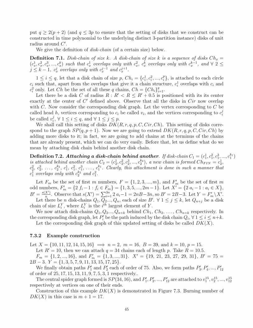
put q ≥ 2(p + 2) (and q ≤ 3p to ensure that the setting of disks that we construct can beconstructed in time polynomial to the underlying distinct 3-partition instance) disks of unitradius around C ′.

We give the definition of disk-chain (of a certain size) below.

Definition 7.1. Disk-chain of size k. A disk-chain of size k is a sequence of disks Chx =(c1x, c

2x, c

3x, ..., c

kx) such that c1x overlaps only with c2x, ckx overlaps only with ck−1x , and ∀ 2 ≤

j ≤ k − 1, cjx overlaps only with cj−1x and cj+1x .

1 ≤ i ≤ q, let that a disk chain of size p, Chi = c1i , c2i , ..., cpi , is attached to each circle

ci such that, apart from the overlaps that give it a chain structure, c1i overlaps with ci andc2i only. Let Ch be the set of all these q chains, Ch = Chiqi=1.

Let there be a disk C of radius R : R′ < R ≤ R′ + 0.5 is positioned with its its centerexactly at the center of C ′ defined above. Observe that all the disks in Cir now overlapwith C. Now consider the corresponding disk graph. Let the vertex corresponding to C becalled head h, vertices corresponding to ci be called vi, and the vertices corresponding to cjibe called vji , ∀ 1 ≤ i ≤ q, and ∀ 1 ≤ j ≤ p.

We shall call this setting of disks DK(R, r, q, p, C, Cir, Ch). This setting of disks corre-spond to the graph SP (q, p + 1). Now we are going to extend DK(R, r, q, p, C, Cir, Ch) byadding more disks to it; in fact, we are going to add chains at the terminus of the chainsthat are already present, which we can do very easily. Before that, let us define what do wemean by attaching disk chain behind another disk chain.

Definition 7.2. Attaching a disk-chain behind another. If disk-chain C1 = (c11, c21, c

31, ..., c

k11 )

is attached behind another chain C2 = (c12, c22, c

32, ..., c

k22 ), a new chain is formed ChFIN = c12,

c22, c32, . . . , c

k22 , c11, c

21, c31, . . . , c

k11 . Clearly, this attachment is done in such a manner that

c11 overlaps only with ck22 and c21.

Let Fm be the set of first m numbers, F = 1, 2, 3, ...,m, and F ′m be the set of first modd numbers, F ′m = 2 fi−1 : fi ∈ Fm = 1, 3, 5, ..., 2m−1. Let X ′ = 2 ai−1 : ai ∈ X,B′ = s(X′)

n. Observe that s(X ′) =

∑3ni=1 2 ai−1 = 2nB−3n, so B′ = 2B−3. Let Y = F ′m\X ′.

Let there be n disk-chains Q1, Q2..., Qn, each of size B′. ∀ 1 ≤ j ≤ k, let Qn+j be a diskchain of size LYi , where LYi is the ith largest element of Y .

We now attach disk-chains Q1, Q2..., Qn+k behind Ch1, Ch2, . . . , Chn+k respectively. Inthe corresponding disk graph, let P ′i be the path induced by the disk chain Qi, ∀ 1 ≤ i ≤ n+k.

Let the corresponding disk graph of this updated setting of disks be called DK(X).

7.3.2 Example construction

Let X = 10, 11, 12, 14, 15, 16 =⇒ n = 2, m = 16, B = 39, and k = 10, p = 15.Let R′ = 10, then we can attach q = 34 chains each of length p. Take R = 10.5.Fm = 1, 2, ..., 16, and F ′m = 1, 3, ..., 31. X ′ = 19, 21, 23, 27, 29, 31, B′ = 75 =

2B − 3. Y = 1, 3, 5, 7, 9, 11, 13, 15, 17, 25.We finally obtain paths P ′1 and P ′2 each of order of 75. Also, we form paths P ′3, P

′4, ..., P

′12

of order of 25, 17, 15, 13, 11, 9, 7, 5, 3, 1 respectively..The central spider graph formed is SP (34, 16), and P ′1, P

′2, ..., P

′12 are attached to v151 , v

152 , ..., v

1512

respectively at vertices on one of their ends.Construction of this example DK(X) is demonstrated in Figure 7.3. Burning number of

DK(X) in this case is m+ 1 = 17.

45

v156 Q6

v157 Q7

v158 Q8

v159Q9

v1510Q10v1511

Q11v1512

Q12

v151 Q1

v152 Q2

v153 Q3

v154Q4

v155Q5

Figure 7.3: Construction of example DK(X).

7.3.3 NP-Completeness

Observe that G can be burnt optimally only if P ′1, P′2, ..., P

′n+k can be broken into paths of

length in F ′m iff P ′1, . . . , P′n can be broken into the subpaths W1,W2, . . . ,W3n of lengths in

X ′ as per the distinct 3-partition problem. Let the final set of subpaths that we desire bePP = W1,W2, . . . ,W3n, Pn+1, . . . , Pn+k. We have that |P | = m. Let ri (∀ 2 ≤ i ≤ m + 1)be the middle vertex on the (i− 1)th largest subpath in PP . Let r1 be the head vertex h ofthe spider graph SP (q, p+ 1) induced by DK(R, r, q, p, C, Cir, Ch). r1 will be able to burnSP (q, p + 1) because p = m − 1. So we have that the graph can be burned by the burningsequence S ′ = (r1, r2, . . . , rm+1) of length m+ 1. Hence we have Lemma 7.6 as follows.

Lemma 7.6. b(DK(X)) ≤ m+ 1.

In Lemma 7.7, we show that the first fire source must be placed at r0, which is stated asfollows.

Lemma 7.7. The first fire source must be placed at r0 (the head vertex h).

Proof. Let for contradiction that the first fire source is not placed at h, an we can still burnDK(X) in m + 1 time steps. From here, we have that r0 will not be able to burn at leastq − 1 leaf nodes of SP (q, p + 1) induced by DK(R, r, q, p, C, Cir, Ch). According to ourconstruction, we only have n+ k < m = p+ 1 subpaths (Qi’s) attached to SP (q, p+ 1). Sowe have that more than p+ 1 unburned leaf nodes are not attached to any subpaths.

Any fire source r2, ..., rm+1 will not be able to burn more than one leaf nodes of SP (q, p+1)because distance between any two leaf nodes is 2(p + 1) = 2m. So even if we ignore thoseunburned leaf nodes which are attached to some subpath (Qi), we have that all the firesources r2, ..., rm+1 together will not be able to burn SP (q, p+ 1). This is a contradiction toour assumption because DK(X) will not be burned in m+ 1 time steps.

Now we have that the path forest induced by P ′1, P′2, . . . , P

′n+k which is exactly same as

the path forest P ′′ of IG(X) that we constructed in Section 7.1. So it follows triviallyby the arguments similar to those in the proofs of Lemma 7.5 and Theorem 7.1 that (1)b(DK(X)) = m+ 1, and (2) the optimal burning of DK(X) is NP-Complete. Therefore, wehave Lemma 7.8 and Theorem 7.3 as follows.

46

Lemma 7.8. b(DK(X)) = m+ 1.

Theorem 7.3. Burning disk graphs optimally is NP-Complete even if the underlying diskrepresentation is given.

7.4 Corollary NP-Hard results

Although the following NP-Completeness have been shown in [7], our constructions in Sec-tion 7.1 imply the corollaries in Section 7.4.1, Section 7.4.2, Section 7.4.3, Section 7.4.4,theconstructions in Section 7.2 imply the corollary in Section 7.4.5, the constructions in Sec-tion 7.3 imply the corollary in Section 7.4.6, and the constructions in Section 7.1 and Sec-tion 7.2 together imply the corollary in Section 7.4.7. Finally, since we have already discussedin Section 4.3 that verification of the correctness of a burning sequence can be done in polyno-mial time, we have that the graph burning problem is NP-Complete which we state formallyin Section 7.4.8 as Corollary 7.9.

7.4.1 Burning trees with maximum degree 3

Corollary 7.2. The optimal burning of trees with maximum degree 3 is NP-Complete.

7.4.2 Burning chordal graphs

Corollary 7.3. The optimal burning of chordal graphs is NP-Complete.

7.4.3 Burning planar graphs

Corollary 7.4. The optimal burning of planar graphs is NP-Complete.

7.4.4 Burning bipartite graphs

Corollary 7.5. The optimal burning of bipartite graphs is NP-Complete.

7.4.5 Burning path forests

Corollary 7.6. The optimal burning of path forests is NP-Complete.

7.4.6 Burning spider graphs

Corollary 7.7. The optimal burning of spider graphs is NP-Complete.

7.4.7 Burning forests

Corollary 7.8. The optimal burning of forests is NP-Complete.

47

7.4.8 NP-Completeness of general graph burning

Corollary 7.9. The optimal burning of general graphs is an NP-Complete problem.

7.5 Summary of this chapter

We utilize the distinct 3-partition problem to reduce to the burning of interval graphs,permutation graphs, and disk graphs. Several graph classes show their burning propertiesto be NP-Complete directly from our constructions, such as trees, forests, chordal graphs,planar graphs, bipartite graphs, path forests, and spider graphs.

48

Chapter 8

Easy burning subproblems

Not much work has been done which gave algorithms for easy (polynomial time) burning ofgraph classes. This chapter includes the findings which show that optimal burning can beperformed on certain graph classes in polynomial time.

8.1 Burning path or cycle (already discussed)

We have already discussed in Section 5.1 that a simple path or cycle can be burned optimallyin polynomial time.

8.2 Burning split graphs

8.2.1 Burning connected split graphs

If the clique C and the independent set I are given for an arbitrary split graph (see Sec-tion 2.4.7) G, then we can burn a connected split graph in two or three steps [35]. Algo-rithm 8.1 shows how to burn a connected split graph optimally in polynomial time.

Algorithm 8.1. Given the input (G, C, I), where G is the input connected split graph, C(represents the clique) and I (represents the the independent set), both are subsets of G.V ,perform the following steps.

Step 1. Time step t = 0.B stores the set of vertices which are burned, initially B = φ. S will store an optimal burningsequence of G, initially S = φ.

Stage 2. Time step t = 1.S = c where c is an arbitrary vertex in C, preferably adjacent to at least one vertex in I.B = c. If B = G.V , then return S.

Stage 3. Time step t = 2.S = S ∪ i, where i is an arbitrary unburned vertex in I (preferably, such that i is notconnected to the same vertex in C as S[|S|]) or C. B = B ∪ i ∪G.Adj[B].If B = G, then return S.

Stage 4. Time step t = 3.S = S ∪ i, where i is an arbitrary unburned vertex in I. B = B ∪ i ∪G.Adj[B].

49

c1 = y2

c2 = y3c3

i = y1

Figure 8.1: If the first fire source is placed on i, then the burning sequence is i, c1, c2. If, otherwise, the firstfire source is placed on c1 (for example), then the burning sequence is c1, i

Return S.

Algorithm 8.1 runs in linear time, given that C and I are computed already. For aconnected split graph G, the burning number b(G) is 2 or 3. It is interesting to observethat even if the split graph is not a connected graph, then also we can burn the graph inpolynomial time O(n), given that the first fire source is placed in C.

8.2.2 Burning general split graphs

Theorem 8.1. For an arbitrary split graph G, the first fire source in an optimal burningsequence should be placed on c, an arbitrary vertex in C (representing the clique), a subgraphof G.V .

Proof. General construction: LetG be a split graph of n vertices such that C = c1, c2, c3, ..., cn−1is a complete subgraph of G of size n−1, and I = i is the independent set excerpt of G. i isnot connected to any vertex in G. Let the optimal burning sequence be S ′ = (y1, y2, y3, ..., yk′)be of k′ vertices. Consider for contradiction that the fire source y1 is placed on i, and yet weare able to burn G in the mininimum possible time steps.

Example construction and solution: Let n = 4. When y1 is placed on i, a burningsequence required to burn G is (i, c1, c2). This is shown in figure 0.2.

On the other hand, if y1 were placed on c1, an arbitrary vertex in C, a burning sequencerequired to burn G is (c1, i).

Given that the vertices of I are connected to atmost one vertex in C, then in an optimalburning sequence, we can put the first fire source on a vertex in I iff there are atmost 2vertices in I which are disconnected from C. If otherwise the vertices of I are connected tomore than one vertices of C, then in an optimal burning sequence, we can put the first firesource on a vertex in I iff there are atmost 3 vertices in I which are disconnected from C.

Theorem 8.1 lays the foundation of algorithm Algorithm 8.2, which computes an optimalburning sequence for disconnected split graphs in O(n).

Algorithm 8.2. Given the input (G, C, I), where G is a connected split graph, C representsthe clique, C ⊆ G.V , and I represents the independent set in G, I ⊆ G.V , perform thefollowing steps.

Step 1. Time step t = 0.B stores the set of vertices which are burned, initially B = φ. S will store an optimal burningsequence of G, initially S = φ.

50

Stage 2. Time step t = 1.S = c where c is an arbitrary vertex in C, preferably adjacent to at least one vertex in I.B = c. If B = G.V , then return S.

Stage 3. Time step t = 2.S = S ∪ i, where i is an arbitrary unburned vertex in I (preferably, such that i is notconnected to the same vertex in C as S[|S|]) or C. B = B ∪ i ∪G.Adj[B].If B = G, then return S.

Stage 4. Perform the following steps until B = G.Stage 4.1. Time step t = t+ 1.

S = S ∪ i, where i is an arbitrary unburned vertex in I. B = B ∪ i ∪G.Adj[B].

Stage 5. Return S.

8.3 Burning cographs

Refer to the definition of cographs in Section 2.4.3. In a cograph G, each vertex in G isatmost at a distance 2 or 3 from v, an arbitrary vertex in G [35]. Hence we can burn acograph in atmost 3 steps.

8.4 Summary of this chapter

In this chapter, we visit graph burning on several graph classes, especially those on whichdetermining the burning number is easy. Although graph burning can be modelled on severalgraph classes in polynomial time, it remains NP-Hard on general graphs; it is NP-Hard evenfor many of those graph classes for which several problems, (which are NP-Hard to solve forgeneral graphs), are straightforward to solve.

51

Chapter 9

Approximating the burning sequence

9.1 Approximation for general graphs

Bessy et. al. [7] have given a 3-approximation algorithm for burning of an arbitrary graph.Algorithm 9.1 (in combination with Procedure 9.1) is able to compute a burning sequencefor a graph G in O(n3) time, where n = |G.V |.

Procedure 9.1. Given the input (G, k, S) where G is the input graph, k is a positive integer,and S is a burning sequence of size k − 1, perform the following steps.

Stage 1. xk = maxmind(u,xj)k−j+1

: j ∈ [1 : i− 1] : u ∈ G.V .Stage 2. S = S ∪s/ (xk). Return S.

Algorithm 9.1. Given the input graph G, perform the following steps.

Stage 1. x1 = some arbitrary vertex. S = (x1).Stage 2. ∀ k ≥ 2, perform the following steps.Stage 2.1. Invoke Procedure 9.1 by passing the input (G, k, S) and store the return

value in S. If S satisfies eq. (4.1), then stop and return S.

We show in Lemma 9.1 and Theorem 9.1 [7] that the burning sequence generated byAlgorithm 9.1 is a burning sequence within 3-approximation. It means that (since graphburning is a minimization problem) if Algorithm 9.1 generates a burning sequence of lengthk, then an optimal burning sequence (generated by Algorithm 5.2) of the subject graph Gshall contain at least k

3fire sources.

Lemma 9.1. Let S = (x1, x2, x3, ..., xk) be a burning sequence returned by procedure 9.1for an input graph G. If S is not able to burn G completely (that is, if S does not satisfyEquation (4.1)), then b(G) ≥

⌈k3

⌉+ 1.

Proof. If S does not satisfy Equation (4.1), then ∃ a vertex u such that

mindist(u, xj)k − j + 1

: j ∈ [k]≥ 1

.∀ i, j ∈ [k], i < j, we have that dist(i, j) ≥ k − j + 1 > k − j. Now ∵ j > i, we have that

k − j >⌈k−j2

⌉+⌈k−i2

⌉, we obtain that the k sets

52

Nd k−12e[x1], Nd k−2

2e[x2], Nd k−3

2e[x3], ..., N0[xk]

are pairwise disjoint.Now let (for contradiction) that a burning sequence of length S ′ = (y1, y2, y3, ..., yk′) of

length k′ is able to burn G, where k′ ≤⌊k3

⌋.

∵ the “half” neighbourhood of the first⌊k3

⌋+1 fire sources is more than the neighbourhood

of the first fire source (the fire source with the maximum neighbourhood reachability) that is,⌈k −

⌈k3

⌉− 1

2

⌉≥⌊k

3

⌋− 1 ≥ k′ − 1,

then each of the (first)⌊k3

⌋+ 1 sets

Nd k−12e[x1], Nd k−2

2e[x2], Nd k−3

2e[x3], ..., N

⌈k−⌈

k3

⌉−1

2

⌉[x⌈ k3

⌉+1

]contain at least one element from S ′. ∵ all these sets are pairwise disjoint, we obtain thecontradiction to our assumption because S ′ will not be able to burn G. So S ′ must containat least one more fire source.

Theorem 9.1. Let S = (x1, x2, x3, ..., xk) be a burning sequence returned by Algorithm 9.1,then b(G) ≥ k

3.

Proof. If Algorithm 9.1 returns a burning sequence of length k, then procedure 24 must nothave been able to burn G with k − 1 fire sources.=⇒ (from Lemma 9.1) b(G) ≥

⌈k−13

⌉+ 1 ≥ k

3.

9.2 How close can we approximate?

Let that for a given arbitrary graph G, S = (x1, x2, x3, ..., xk) be a burning sequence returnedby an arbitrary approximation algorithm A in polynomial time. If for a pair of fire sourcesxi, xj their neighbourhoods are disjoint then the following expression satisfies.∣∣G.Nk−i[xi] ∩G.Nk−j[xj]

∣∣ = 0.

If for a pair of fire sources xi, xj it is observed that the f th fraction (0 ≤ f ≤ 1) of theirneighbourhoods are disjoint then the following expression satisfies.∣∣G.Ndf×(k−i)e[xi] ∩G.Ndf×(k−j)e[xj]∣∣ = 0.

So, “half” neighbourhoods (where f = 12) of any two distinct fire sources xi and xj are

disjoint iff ∣∣∣ G.N⌈ k−i2

⌉[xi] ∩G.N⌈ k−j2

⌉[xj] ∣∣∣ = 0.

By Lemma 5.1 (in Section 5.2), we have that b(SP (s, r)) = r + 1 if s ≥ r; if s ≥ r + 2,then the first fire source y1 of the optimal burning sequence S ′ = (y1, y2, y3, ..., yk′) must beplaced on its head node c.

53

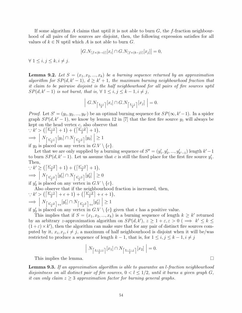
If some algorithm A claims that uptil it is not able to burn G, the f -fraction neighbour-hood of all pairs of fire sources are disjoint, then, the following expression satisfies for allvalues of k ∈ N uptil which A is not able to burn G.∣∣G.Ndf×(k−i)e[xi] ∩G.Ndf×(k−j)e[xj]∣∣ = 0,

∀ 1 ≤ i, j ≤ k, i 6= j.

Lemma 9.2. Let S = (x1, x2, ..., xk) be a burning sequence returned by an approximationalgorithm for SP (d, k′ − 1), d ≥ k′ + 1, the maximum burning neighbourhood fraction thatit claim to be pairwise disjoint is the half neighbourhood for all pairs of fire sources uptilSP (d, k′ − 1) is not burnt, that is, ∀ 1 ≤ i, j ≤ k − 1, i 6= j,∣∣∣ G.N⌈ k−i

2

⌉[xi] ∩G.N⌈ k−j2

⌉[xj] ∣∣∣ = 0.

Proof. Let S ′ = (y1, y2, ..., yk′) be an optimal burning sequence for SP (∞, k′−1). In a spidergraph SP (d, k′ − 1), we know by lemma 12 in [7] that the first fire source y1 will always bekept on the head vertex c, also observe that∵ k′ >

(⌈k′−12

⌉+ 1)

+(⌈

k′−22

⌉+ 1),

=⇒∣∣∣ N⌈ k′−1

2

⌉[y1] ∩N⌈ k′−22

⌉[y2] ∣∣∣ ≥ 1

if y2 is placed on any vertex in G.V \ c.Let that we are only supplied by a burning sequence of S ′′ = (y′1, y

′2, ..., y

′k′−1) length k′−1

to burn SP (d, k′− 1). Let us assume that c is still the fixed place for the first fire source y′1.Then,∵ k′ ≥

(⌈k′−22

⌉+ 1)

+(⌈

k′−32

⌉+ 1),

=⇒∣∣∣ N⌈ k′−2

2

⌉[y′1] ∩N⌈ k′−32

⌉[y′2] ∣∣∣ ≥ 0

if y′2 is placed on any vertex in G.V \ c.Also observe that if the neighbourhood fraction is increased, then,

∵ k′ >(⌈

k′−12

⌉+ ε+ 1

)+(⌈

k′−22

⌉+ ε+ 1

),

=⇒∣∣∣ N⌈ k′−2

2

⌉+ε

[y′1] ∩N⌈ k′−32

⌉+ε

[y′2]∣∣∣ ≥ 1

if y′2 is placed on any vertex in G.V \ c given that ε has a positive value.This implies that if S = (x1, x2, ..., xk) is a burning sequence of length k ≥ k′ returned

by an arbitrary z-approximation algorithm on SP (d, k′), z ≥ 1 + ε, ε > 0 ( =⇒ k′ ≤ k ≤(1 + ε)×k′), then the algorithm can make sure that for any pair of distinct fire sources com-puted by it, xi, xj, i 6= j, a maximum of half neighbourhood is disjoint when it will be/wasrestricted to produce a sequence of length k − 1, that is, for 1 ≤ i, j ≤ k − 1, i 6= j∣∣∣ N⌈ k−1−i

2

⌉[x1] ∩N⌈ k−1−j2

⌉[x2] ∣∣∣ = 0.

This implies the lemma.

Lemma 9.3. If an approximation algorithm is able to guarantee an l-fraction neighbourhooddisjointness on all distinct pair of fire sources, 0 < l ≤ 1/2, until it burns a given graph G,it can only claim z ≥ 3 approximation factor for burning general graphs.

54

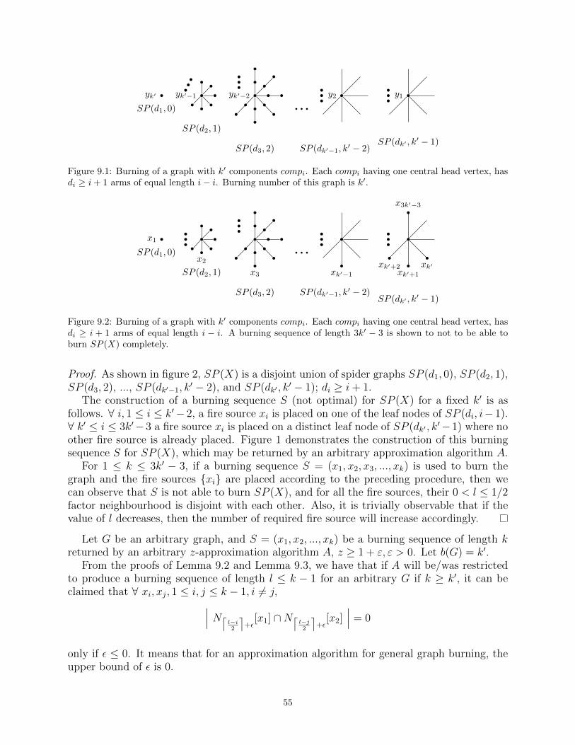
yk′ yk′−1 yk′−2 y2 y1

SP (d1, 0)

SP (d2, 1)

SP (d3, 2) SP (dk′−1, k′ − 2)

SP (dk′ , k′ − 1)

Figure 9.1: Burning of a graph with k′ components compi. Each compi having one central head vertex, hasdi ≥ i + 1 arms of equal length i− i. Burning number of this graph is k′.

x1

x2

x3 xk′−1xk′

xk′+1

xk′+2

x3k′−3

SP (d1, 0)

SP (d2, 1)

SP (d3, 2) SP (dk′−1, k′ − 2)

SP (dk′ , k′ − 1)

Figure 9.2: Burning of a graph with k′ components compi. Each compi having one central head vertex, hasdi ≥ i + 1 arms of equal length i − i. A burning sequence of length 3k′ − 3 is shown to not to be able toburn SP (X) completely.

Proof. As shown in figure 2, SP (X) is a disjoint union of spider graphs SP (d1, 0), SP (d2, 1),SP (d3, 2), ..., SP (dk′−1, k

′ − 2), and SP (dk′ , k′ − 1); di ≥ i+ 1.

The construction of a burning sequence S (not optimal) for SP (X) for a fixed k′ is asfollows. ∀ i, 1 ≤ i ≤ k′− 2, a fire source xi is placed on one of the leaf nodes of SP (di, i− 1).∀ k′ ≤ i ≤ 3k′−3 a fire source xi is placed on a distinct leaf node of SP (dk′ , k

′−1) where noother fire source is already placed. Figure 1 demonstrates the construction of this burningsequence S for SP (X), which may be returned by an arbitrary approximation algorithm A.

For 1 ≤ k ≤ 3k′ − 3, if a burning sequence S = (x1, x2, x3, ..., xk) is used to burn thegraph and the fire sources xi are placed according to the preceding procedure, then wecan observe that S is not able to burn SP (X), and for all the fire sources, their 0 < l ≤ 1/2factor neighbourhood is disjoint with each other. Also, it is trivially observable that if thevalue of l decreases, then the number of required fire source will increase accordingly.

Let G be an arbitrary graph, and S = (x1, x2, ..., xk) be a burning sequence of length kreturned by an arbitrary z-approximation algorithm A, z ≥ 1 + ε, ε > 0. Let b(G) = k′.

From the proofs of Lemma 9.2 and Lemma 9.3, we have that if A will be/was restrictedto produce a burning sequence of length l ≤ k − 1 for an arbitrary G if k ≥ k′, it can beclaimed that ∀ xi, xj, 1 ≤ i, j ≤ k − 1, i 6= j,∣∣∣ N⌈ l−i

2

⌉+ε

[x1] ∩N⌈ l−j2

⌉+ε

[x2]∣∣∣ = 0

only if ε ≤ 0. It means that for an approximation algorithm for general graph burning, theupper bound of ε is 0.

55

This is the maximum that A can claim for a general graph. Let that A is able to guaranteethis. It means that if G is not burnt completely and ε ≤ 0, then A guarantees thatNd k−1

2e[x1], Nd k−2

2e[x2], Nd k−3

2e[x3], ..., N0[xk] are pairwise disjoint, and

∵

⌈k−⌈

k3

⌉−1

2

⌉≥⌊k3

⌋− 1,

=⇒ b(G) ≤⌊k3

⌋+ 1 (by Lemma 9.1).

=⇒ z ≥ 3 =⇒ ε = 2 (by Theorem 9.1).These properties allow us to suggest that graph burning may be hard to approximate

better than the 3-approximation ratio, which we formally state as Conjecture 9.1 as follows.

Conjecture 9.1. A maximum of 3-approximation is possible in polynomial time to computeburning number of general graphs.

If it is a necessary attribute for an approximation algorithm for burning general graphsto claim a neighbourhood factor disjointness between each pair of fire sources in the burningsequence S = (x1, x2, ..., xk) returned by it, then a maximum of 3-approximation is possiblein polynomial time to compute burning number of general graphs.

9.3 Approximating the burning of connected interval graphs

We discussed in Section 3.4.1 that if P is the diameter of an interval graph G, then allthe other vertices in G, that is, the vertices in G \ P , are connected to at least one vertexin P by a single edge. We discussed in Section 5.1 that we can burn a path optimally inpolynomial time using Algorithm 5.1. Following from this we discussed in Section 7.1.1 thatthe burning number of an interval graph G b(P ) ≤ b(G) ≤ b(P )+1. We showed in Section 7.1that determining whether b(G) = b(P ) is NP-Complete. We describe Algorithm 9.2 asfollows, which is able to burn an interval graph G within b(G) + 1. We have used theAlgebraic-Floyd-Warshall [38] to compute P , the diameter of G, which is a shortestpath of maximum length in G.

Algorithm 9.2. Given an interval graph G, perform the following steps.

Stage 1. F = a set of shortest paths between all pairs of vertices from the Algebraic-Floyd-Warshall algorithm. P = a path of maximum length in F .

Stage 2. Invoke Algorithm 5.1 by passing (G,P ) as input, store the return value inS = (x1, x2, . . . , xk).

Stage 3. If S is not able to burnG completely, that is, if S does not satisfy Equation (4.1),then v = an arbitrary vertex in G.V \(G.Nk−1[x1]∪G.Nk−2[x2]∪· · ·∪G.N0[xk]). S = S∪s/v.

Stage 4. Return S.

Time complexity of Algorithm 9.2 is O(n), where n is the number of vertices in G. S isthe burning sequence returned by Algorithm 9.2.

In Section 1.9, we discussed in Theorem 1.1 that no approximation algorithm A canguarantee an approximation ratio RA of less than k + (1/k) if k is the cost of the optimalsolution of a problem P on some input x. If the burning number of a connected interval graphG be k = b(G), Algorithm 9.2 is able to approximate burning of interval graphs within k+1.Thus we get that the approximation ratio for burning interval graphs is RA = k + (1/k).

56

9.4 Summary of this chapter

We describe a 3-approximation algorithm for burning general graphs, as described in [7].Based on some properties of graph burning, we provide a conjecture that graph burningcannot be approximated to a factor less than 3. We also discuss the approximation oninterval graphs, deriving from the properties presented in [35].

57

Chapter 10

Conclusion and future work

10.1 Observations

10.1.1 On graph burning

Discovery of the graph burning and the burning number property was motivated by theworks that were trying to model the spread of an object. This object multiplies and spreadsto nodes through connections.

This object is, so far, related to spread of electronic information in a network, for example,spread of a meme, a gossip, a social contagion, influence or emotion, message, or alarmsthrough a social network. The burning number describes the minimum number of (discrete)time-steps that are able to “infect” the whole network with an object.

10.1.2 Burning versus other problems

Optimal graph burning is proved to be computationally hard on various graph classes. Itis clear with reference to interval graphs, permutation graphs, disk graphs, spider graphs,trees, path forests and several other graph classes that optimal burning of such graph classesis NP-Complete where other problems, which are NP-Complete for general graphs, can besolved in polynomial time. While proving NP-Completeness, we have extensively utilizedthe distinct 3-partition problem, by reducing it to the burning of several graph classes.

Although, burning is easy on some other graph classes such as split graphs and cographs.

10.1.3 Approximating the burning sequence

The 3-approximation algorithm for deriving a burning sequence for an arbitrary graph isbased on the pairwise disjointness of the half neighbourhoods of the fire sources.

Approximating the burning sequence for general graphs better than the factor of 3 maybe computationally hard because pairwise disjointness on more than half neighbourhood ofthe fire sources is not possible on general graphs.

58

10.2 What next?

10.2.1 Discrete mathematics and theoretical algorithm design

So far a few graphs have been shown to be NP-Complete from the burning perspective, afew have been shown to be solvable in polynomial time. Still several of the graph classes areleft to research on, which are useful in various practical scenarios, and determine whetherderiving an optimal burning sequence is solvable polynomially.

We showed that we can approximate burning of interval graphs, which we have shown tobe NP-Complete to solve optimally, within an approximation ratio of 1 + (1/k), but not lessthan this factor. This observation is close enough to the limit imposed by the theorem thatif P 6= NP, then RA ≥ 1 + (1/k) in all cases. Although, the conjecture that P 6= NP remainsunaffected, and we have not proved or disproved it.

10.2.2 Practical implementations

Graph burning has been proposed to model several real-time systems which are complexotherwise.

The graph burning can also be used in several practical scenarios other than spreading amessage, alarm, or contagion. For example, the spread of an infection, virus, etc can also bemodelled using this newly discovered graph procedure. We can model the spread of a “real-life” contagion using graph burning, such as person-to-person spread of a communicableinfection.

The multiplication of the virus inside a host and its behavior of infecting the network oftarget cells may also be modelled very precisely same as how the fire spreads throughout agraph. And then the firefighter problem can be used to simulate the defence of the host body.Similarly, firefighter can also be used in the simulation of the “real-life” social communicationof a disease, where it can be used to model how do or how good can we plan for the defencemechanism, given the constraints such as availability of vaccines, etc by using the minimumresources to save the maximum population.

It might not be very simple and also, may not be exactly same as what we have modelledso far theoretically on static graphs; weights may be involved, time instances may not bediscrete and at equal intervals as we model theoretically. Probabilities with respect to thespread or rescue may also be involved, along with deaths (with probabilities involved). Insuch cases, elimination of cells from the body and people from a real-life social network, whichcan be modelled by elimination of vertices in the graph being modelled. So, this model thatwe propose as one of the probable future works can also be extended to probabilistic ortemporal graphs which may give us better, more precise results based on the “real-life”circumstances.

59

Bibliography

[1] Marek Simon, Ladislav Huraj, Iveta Dirgova Luptakova, and Ji rı Pospıchal. Heuristicsfor spreading alarm throughout a network. Applied Sciences, 9(16), 2019.

[2] Noga. Alon, PaweL. PraLat, and Nicholas. Wormald. Cleaning regular graphs withbrushes. SIAM Journal on Discrete Mathematics, 23(1):233–250, 2009.

[3] Mikhail J. Atallah, Glenn K. Manacher, and J. Urrutia. Finding a minimum independentdominating set in a permutation graph. Discrete Applied Mathematics, 21(3):177 – 183,1988.

[4] Jozsef Balogh, Bela Bollobas, and Robert Morris. Graph bootstrap percolation. RandomStructures and Algorithms, 41(4):413–440, 12 2012.

[5] Siddhartha Banerjee, Aditya Gopalan, Abhik Das, and Sanjay Shakkottai. Epidemicspreading with external agents. IEEE Transactions on Information Theory, 60, 06 2012.

[6] Alan A. Bertossi. Dominating sets for split and bipartite graphs. Information ProcessingLetters, 19(1):37 – 40, 1984.

[7] Stephane Bessy, Anthony Bonato, Jeannette Janssen, Dieter Rautenbach, and ElhamRoshanbin. Burning a graph is hard. Discrete Appl. Math., 232(C):73–87, 2017.

[8] Stephane Bessy, Anthony Bonato, Jeannette Janssen, Dieter Rautenbach, and ElhamRoshanbin. Bounds on the burning number. Discrete Applied Mathematics, 235:16 –22, 2018.

[9] Bela Bollobas, Michal Przykucki, Oliver Riordan, and Julian Sahasrabudhe. On themaximum running time in graph bootstrap percolation. Electronic Journal of Combi-natorics, 24, 05 2017.

[10] Anthony Bonato, Jeannette Janssen, and Elham Roshanbin. How to burn a graph.Internet Mathematics, 12(1-2):85–100, 2016.

[11] Anthony Bonato and Shahin Kamali. Approximation Algorithms for Graph Burning.In T.V. Gopal and Junzo Watada, editors, Theory and Applications of Models of Com-putation, Lecture Notes in Computer Science, pages 74–92, Cham, 2019. Springer Inter-national Publishing.

[12] Anthony Bonato and Thomas Lidbetter. Bounds on the burning numbers of spiders andpath-forests. Theoretical Computer Science, 794:12 – 19, 2019. Special Issue on Theoryand Applications of Graph Searching.

60

[13] Anna Bretscher, Derek Corneil, Michel Habib, and Christophe Paul. A simple lineartime lexbfs cograph recognition algorithm. SIAM Journal on Discrete Mathematics,22(4):1277–1296, 2008.

[14] J Chalupa, P L Leath, and G R Reich. Bootstrap percolation on a bethe lattice. Journalof Physics C: Solid State Physics, 12(1):L31–L35, jan 1979.

[15] Brent N. Clark, Charles J. Colbourn, and David S. Johnson. Unit disk graphs. DiscreteMathematics, 86(1):165 – 177, 1990.

[16] Thomas H. Cormen, Charles E. Leiserson, Ronald L. Rivest, and Clifford Stein. Intro-duction to Algorithms. The MIT Press, 3 edition, 2009.

[17] D. G. Corneil, Y. Perl, and L. K. Stewart. A linear recognition algorithm for cographs.SIAM Journal on Computing, 14(4):926–934, 1985.

[18] D.G. Corneil, H. Lerchs, and L.Stewart Burlingham. Complement reducible graphs.Discrete Applied Mathematics, 3(3):163 – 174, 1981.

[19] Peter Damaschke. Induced subgraphs and well-quasi-ordering. Journal of Graph Theory,14(4):427–435, 1990.

[20] Subrata Dasgupta. It Began with Babbage: The Genesis of Computer Science. OxfordUniversity Press, feb 2014.

[21] Pedro Domingos and Matt Richardson. Mining the network value of customers. InProceedings of the Seventh ACM SIGKDD International Conference on Knowledge Dis-covery and Data Mining, KDD-01, pages 57–66, New York, NY, USA, 2001. Associationfor Computing Machinery.

[22] Ralph Faudree and Ralph Faudree. Weak saturation numbers for graphs. CongressusNumerantium, 01 2013.

[23] Fedor V. Fomin, Pinar Heggernes, and Erik Jan van Leeuwen. The firefighter problemon graph classes. Theoretical Computer Science, 613:38 – 50, 2016.

[24] Michael R. Garey and David S. Johnson. Computers and Intractability: A Guide to theTheory of NP-Completeness. W. H. Freeman & Co., USA, 1979.

[25] P. C. Gilmore and A. J. Hoffman. A characterization of comparability graphs and ofinterval graphs. Canadian Journal of Mathematics, 16:539–548, 1964.

[26] Emeric Gioan and Christophe Paul. Split decomposition and graph-labelled trees: Char-acterizations and fully dynamic algorithms for totally decomposable graphs. DiscreteApplied Mathematics, 160(6):708 – 733, 2012. Fourth Workshop on Graph Classes,Optimization, and Width Parameters Bergen, Norway, October 2009.

[27] Martin Charles Golumbic. Algorithmic Graph Theory and Perfect Graphs (Annals ofDiscrete Mathematics, Vol 57). North-Holland Publishing Co., NLD, 2004.

[28] Michel Habib and Christophe Paul. A simple linear time algorithm for cograph recogni-tion. Discrete Applied Mathematics, 145(2):183 – 197, 2005. Structural Decompositions,Width Parameters, and Graph Labelings.

61

[29] Peter L. Hammer and Bruno Simeone. The splittance of a graph. Combinatorica,1(3):275–284, Sep 1981.

[30] B. Hartnell. Firefighter! an application of domination. the 24th Manitoba Conference onCombinatorial Mathematics and Computing, University of Minitoba, Winnipeg, Cadada,1995, 1995.

[31] Heather Hulett, Todd G. Will, and Gerhard J. Woeginger. Multigraph realizations ofdegree sequences: Maximization is easy, minimization is hard. Operations ResearchLetters, 36(5):594 – 596, 2008.

[32] Louis Ibarra. Computing the clique-separator graph for an interval graph in linear time.Information Processing Letters, 124:21 – 25, 2017.

[33] Shahin Kamali, Avery Miller, and Kenny Zhang. Burning two worlds: Algorithms forburning dense and tree-like graphs, 2019.

[34] Shahin Kamali, Avery Miller, and Kenny Zhang. Burning two worlds. In Alexan-der Chatzigeorgiou, Riccardo Dondi, Herodotos Herodotou, Christos Kapoutsis, YannisManolopoulos, George A. Papadopoulos, and Florian Sikora, editors, SOFSEM 2020:Theory and Practice of Computer Science, pages 113–124, Cham, 2020. Springer Inter-national Publishing.

[35] Anjeneya Swami Kare and I. Vinod Reddy. Parameterized Algorithms for Graph Burn-ing Problem. In Charles J. Colbourn, Roberto Grossi, and Nadia Pisanti, editors,Combinatorial Algorithms, Lecture Notes in Computer Science, pages 304–314, Cham,2019. Springer International Publishing.

[36] David Kempe, Jon Kleinberg, and Eva Tardos. Maximizing the spread of influencethrough a social network. In Proceedings of the Ninth ACM SIGKDD InternationalConference on Knowledge Discovery and Data Mining, KDD-03, pages 137–146, NewYork, NY, USA, 2003. Association for Computing Machinery.

[37] David Kempe, Jon Kleinberg, and Eva Tardos. Influential nodes in a diffusion modelfor social networks. In Proceedings of the 32nd International Conference on Automata,Languages and Programming, ICALP-05, pages 1127–1138, Berlin, Heidelberg, 2005.Springer-Verlag.

[38] Jeremy V. Kepner and John R. (John R.) Gilbert. Graph algorithms in the language oflinear algebra. Software, environments, and tools ; 22. Society for Industrial and AppliedMathematics, 2011.

[39] Adam D. I. Kramer, Jamie E. Guillory, and Jeffrey T. Hancock. Experimental evi-dence of massive-scale emotional contagion through social networks. Proceedings of theNational Academy of Sciences, 111(24):8788–8790, 2014.

[40] George S. Lueker and Kellogg S. Booth. A linear time algorithm for deciding intervalgraph isomorphism. J. ACM, 26(2):183–195, April 1979.

[41] M. V. Marathe, H. Breu, H. B. Hunt, S. S. Ravi, and D. J. Rosenkrantz. Simpleheuristics for unit disk graphs. Networks, 25(2):59–68, March 1995.

62

[42] Madhav V. Marathe, R. Ravi, and C. Pandu Rangan. Generalized vertex covering ininterval graphs. Discrete Applied Mathematics, 39(1):87 – 93, 1992.

[43] S Mckeil. Chip firing cleaning processes. mathesis, Dalhousie University, 2007.

[44] Luigi Frederico Menabrea. Scientific Memoirs, volume 3, chapter Sketch of the analyticalengine invented by Charles Babbage, Esq, pages 666–731. Taylor and Francis, 1843.

[45] Margaret-Ellen Messinger, Richard Nowakowski, and Pawel Pralat. Cleaning a networkwith brushes. Theoretical Computer Science, 399:191–205, 06 2008.

[46] Elchanan Mossel and Sebastien Roch. On the submodularity of influence in socialnetworks. In Proceedings of the Thirty-Ninth Annual ACM Symposium on Theory ofComputing, STOC-07, pages 128–134, New York, NY, USA, 2007. Association for Com-puting Machinery.

[47] Haiko Muller. Hamiltonian circuits in chordal bipartite graphs. Discrete Mathematics,156(1):291 – 298, 1996.

[48] Stephan Olariu. An optimal greedy heuristic to color interval graphs. InformationProcessing Letters, 37(1):21 – 25, 1991.

[49] G. Ramalingam and C.Pandu Rangan. A unified approach to domination problems oninterval graphs. Information Processing Letters, 27(5):271 – 274, 1988.

[50] R. Ravi, Madhav V. Marathe, and C. Pandu Rangan. An optimal algorithm to solvethe all-pair shortest path problem on interval graphs. Networks, 22(1):21–35, 1992.

[51] Matthew Richardson and Pedro Domingos. Mining knowledge-sharing sites for viralmarketing. In Proceedings of the Eighth ACM SIGKDD International Conference onKnowledge Discovery and Data Mining, KDD-02, pages 61–70, New York, NY, USA,2002. Association for Computing Machinery.

[52] Laurence Sigler. Fibonacci’s Liber Abaci. Springer New York, 2002.

[53] Marek Simon, Ladislav Huraj, Dirgova LuptakovaIveta, and Jiri Pospichal. How to burna network or spread alarm. MENDEL, 25(2):11–18, Dec. 2019.

[54] A. M. Turing. On computable numbers, with an application to the entscheidungsprob-lem. Proceedings of the London Mathematical Society, s2-42(1):230–265, 1937.

63