Bridge Deck Integrity Measurements for Asset … Deck Integrity Measurements for Asset Management...

Bridge Deck Integrity Measurements for Asset Management

Final ReportJune 2009

Sponsored byUniversity Transportation Centers Program,U.S. Department of Transportation(MTC Project 2007-03)

About the MTC

The mission of the University Transportation Centers (UTC) program is to advance U.S. technology and expertise in the many disciplines comprising transportation through the mechanisms of education, research, and technology transfer at university-based centers of excellence. The Midwest Transportation Consortium (MTC) is a Tier 1 University Transportation Center that includes Iowa State University, the University of Iowa, and the University of Northern Iowa. Iowa State University, through its Institute for Transportation (InTrans), is the MTC’s lead institution.

Disclaimer Notice

The contents of this report reflect the views of the authors, who are responsible for the facts and the accuracy of the information presented herein. The opinions, findings and conclusions expressed in this publication are those of the authors and not necessarily those of the sponsors.

The sponsors assume no liability for the contents or use of the information contained in this document. This report does not constitute a standard, specification, or regulation.

The sponsors do not endorse products or manufacturers. Trademarks or manufacturers’ names appear in this report only because they are considered essential to the objective of the document.

Non-discrimination Statement

Iowa State University does not discriminate on the basis of race, color, age, religion, national origin, sexual orientation, gender identity, sex, marital status, disability, or status as a U.S. veteran. Inquiries can be directed to the Director of Equal Opportunity and Diversity, (515) 294-7612.

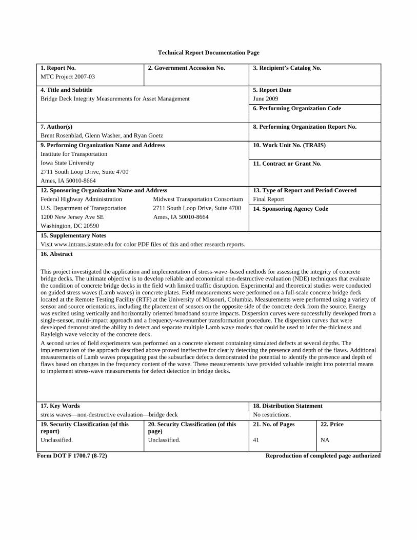
Technical Report Documentation Page

1. Report No. 2. Government Accession No. 3. Recipient’s Catalog No. MTC Project 2007-03

4. Title and Subtitle 5. Report Date Bridge Deck Integrity Measurements for Asset Management June 2009

6. Performing Organization Code

7. Author(s) 8. Performing Organization Report No. Brent Rosenblad, Glenn Washer, and Ryan Goetz 9. Performing Organization Name and Address 10. Work Unit No. (TRAIS) Institute for Transportation Iowa State University 2711 South Loop Drive, Suite 4700 Ames, IA 50010-8664

11. Contract or Grant No.

12. Sponsoring Organization Name and Address 13. Type of Report and Period Covered Federal Highway Administration Midwest Transportation Consortium U.S. Department of Transportation 2711 South Loop Drive, Suite 4700 1200 New Jersey Ave SE Ames, IA 50010-8664 Washington, DC 20590

Final Report 14. Sponsoring Agency Code

15. Supplementary Notes Visit www.intrans.iastate.edu for color PDF files of this and other research reports. 16. Abstract This project investigated the application and implementation of stress-wave–based methods for assessing the integrity of concrete bridge decks. The ultimate objective is to develop reliable and economical non-destructive evaluation (NDE) techniques that evaluate the condition of concrete bridge decks in the field with limited traffic disruption. Experimental and theoretical studies were conducted on guided stress waves (Lamb waves) in concrete plates. Field measurements were performed on a full-scale concrete bridge deck located at the Remote Testing Facility (RTF) at the University of Missouri, Columbia. Measurements were performed using a variety of sensor and source orientations, including the placement of sensors on the opposite side of the concrete deck from the source. Energy was excited using vertically and horizontally oriented broadband source impacts. Dispersion curves were successfully developed from a single-sensor, multi-impact approach and a frequency-wavenumber transformation procedure. The dispersion curves that were developed demonstrated the ability to detect and separate multiple Lamb wave modes that could be used to infer the thickness and Rayleigh wave velocity of the concrete deck. A second series of field experiments was performed on a concrete element containing simulated defects at several depths. The implementation of the approach described above proved ineffective for clearly detecting the presence and depth of the flaws. Additional measurements of Lamb waves propagating past the subsurface defects demonstrated the potential to identify the presence and depth of flaws based on changes in the frequency content of the wave. These measurements have provided valuable insight into potential means to implement stress-wave measurements for defect detection in bridge decks.

17. Key Words 18. Distribution Statement stress waves—non-destructive evaluation—bridge deck No restrictions. 19. Security Classification (of this report)

20. Security Classification (of this page)

21. No. of Pages 22. Price

Unclassified. Unclassified. 41 NA

Form DOT F 1700.7 (8-72) Reproduction of completed page authorized

BRIDGE DECK INTEGRITY MEASUREMENTS FOR ASSET MANAGEMENT

Final Report June 2009

Principal Investigator Brent Rosenblad

Assistant Professor, Department of Civil and Environmental Engineering University of Missouri

Co-Principal Investigator

Glenn Washer Assistant Professor, Department of Civil and Environmental Engineering

University of Missouri

Research Assistant Ryan Goetz

Authors

Brent Rosenblad, Glenn Washer, and Ryan Goetz

Sponsored by a Federal Highway Administration pooled fund study

and the Midwest Transportation Consortium

a U.S. DOT Tier 1 University Transportation Center (MTC Project 2007-03)

A report from Midwest Transportation Consortium

Iowa State University 2711 South Loop Drive, Suite 4700

Ames, IA 50010-8664 Phone: 515-294-8103 Fax: 515-294-0467

www.mtc.iastate.edu

v

TABLE OF CONTENTS

ACKNOWLEDGMENTS ............................................................................................................ IX

EXECUTIVE SUMMARY .......................................................................................................... XI

1. INTRODUCTION .......................................................................................................................1

2. BACKGROUND AND PAST STUDIES ....................................................................................2

3. THEORETICAL STUDIES .........................................................................................................3

4. EXPERIMENTAL STUDIES AT RTF SITE .............................................................................8 4.1 Experimental Methods ...................................................................................................8 4.2 Experimental Results ...................................................................................................11

5. EXPERIMENTAL STUDIES AT MIDWAY SITE .................................................................20 5.1 Experimental Results from Midway Site .....................................................................21

6. CONCLUSIONS ........................................................................................................................27

7. RECOMMENDATIONS FOR FUTURE STUDIES ................................................................28

REFERENCES ..............................................................................................................................29

LIST OF FIGURES

Figure 1. Symmetric and antisymmetric modes for a 20.3 cm (8 in.) thick concrete plate with free boundary conditions .............................................................................................................3

Figure 2. Theoretical symmetric and antisymmetric modes for (a) 7.62 cm (3 in.), (b) 15.27 cm (6 in.), and (c) 30.32 cm (8 in.) thick concrete plates ..........................................................5

Figure 3. Theoretical modal response of symmetric modes plotted in terms of wavelength for 7.62 cm (3 in.), 15.24 cm (6 in.), 20.32 cm (8 in.), and 30.48 cm (12 in.) thick concrete ..6

Figure 4. Theoretical dispersion curves for horizontally polarized shear waves for (a) symmetric modes and (b) antisymmetric modes of 7.62 cm (3 in.), 15.24 cm (6 in.), 20.32 cm (8 in.), and 30.48 cm (12 in.) thick concrete ...................................................................................7

Figure 5. Full-scale bridge deck at the RTF prior to removal from site ..........................................8 Figure 6. Instrumentation used to excite and measure waves at the RTF bridge deck site .............9 Figure 7. Experimental arrangement used to collect measurements at the RTF bridge deck site .10 Figure 8. Phase velocity–frequency contour plot for Case 1: Vertical impact with vertical sensor;

source and receiver on same side .......................................................................................11 Figure 9. Case 1: Experimental dispersion curve with theoretical dispersion curve .....................12 Figure 10. Case 1: Experimental dispersion curve (with theoretical dispersion curve) for first 18

impacts at 0 to 0.91 m (0 to 3 ft) ........................................................................................13 Figure 11. Case 1: Experimental dispersion curve (with theoretical dispersion curve) for last 18

impacts at 0.91 to 1.83 m (3 to 6 ft) ...................................................................................13 Figure 12. Impact-echo measurement with 2.54 cm (1 in.) source-receiver spacing ....................13 Figure 13. Case 2: Experimental dispersion curve with theoretical dispersion curve ...................14 Figure 14. Case 2: Experimental dispersion curve (with theoretical dispersion curve) for first 18


impacts at 0.91 to 1.83 m (3 to 6 ft) ...................................................................................15 Figure 16. Case 3: Experimental dispersion curve with theoretical dispersion curve ...................15 Figure 17. Case 3: Experimental dispersion curve (with theoretical dispersion curve) for first 18


impacts at 0.91 to 1.83 m (3 to 6 ft) ...................................................................................16 Figure 19. Case 4: Experimental dispersion curve with theoretical dispersion curve ...................17 Figure 20. Case 4: Experimental dispersion curve (with theoretical dispersion curve) for first 18


impacts at 0.91 to 1.83 m (3 to 6 ft) ...................................................................................17 Figure 22. Case 5: Experimental dispersion curve (with theoretical dispersion curve) for

horizontally polarized shear waves ....................................................................................18 Figure 23. Case 6: Experimental dispersion curve (with theoretical dispersion curve) for

horizontally polarized shear waves ....................................................................................19 Figure 24. Concrete block with subsurface defects at the Midway site ........................................20 Figure 25. Drawing showing the interior of the Midway block and the locations of subsurface

defects in relation to the block. Numbers shown indicate the depth of the simulated delamination in inches. ......................................................................................................21

Figure 26. Experimental dispersion curve developed from vertical motions for (a) control with no defects and (b) 5.08 cm (2 in.), (c) 7.62 cm (3 in.), and (d) 12.7 cm (5 in.) deep

vii

viii

defects. The theoretical dispersion curves for the control case are also shown. ...............22 Figure 27. Experimental dispersion curve developed from radial motions for (a) control with no

defects and (b) 5.08 cm (2 in.), (c) 7.62 cm (3 in.), and (d) 12.7 cm (5 in.) deep defects. The theoretical dispersion curves for the control case are also shown. .............................23

Figure 28. Experimental dispersion curve developed from SH motions for (a) control with no defects and (b) 5.08 cm (2 in.) and (c) 7.62 cm (3 in.) deep defects. The theoretical dispersion curves for the control case are also shown. ......................................................24

Figure 29. Impact-echo measurements recorded over the defect at a depth of 12.7 cm (5 in.) .....25 Figure 30. Transfer function recorded between hammer and radially oriented sensor separated by

0.97 m with a 12.7 cm deep defect present. The transfer function for the control is also shown. ................................................................................................................................26

Figure 31. Transfer function recorded between hammer and radially oriented sensor separated by 0.97 m with a 7.6 cm deep defect present. The transfer function for the control is also shown. ................................................................................................................................26

ACKNOWLEDGMENTS

The authors would like to thank MTC for sponsoring this research.

ix

xi

EXECUTIVE SUMMARY

This project investigated the application and implementation of stress-wave–based methods for assessing the integrity of concrete bridge decks. The ultimate objective is to develop reliable and economical non-destructive evaluation (NDE) techniques that evaluate the condition of concrete bridge decks in the field with limited traffic disruption. Experimental and theoretical studies were conducted on guided stress waves (Lamb waves) in concrete plates. Field measurements were performed on a full-scale concrete bridge deck located at the Remote Testing Facility (RTF) at the University of Missouri, Columbia. Measurements were performed using a variety of sensor and source orientations, including the placement of sensors on the opposite side of the concrete deck from the source. Energy was excited using vertically and horizontally oriented broadband source impacts. Dispersion curves were successfully developed from a single-sensor, multi-impact approach and a frequency-wavenumber transformation procedure. The dispersion curves that were developed demonstrated the ability to detect and separate multiple Lamb wave modes that could be used to infer the thickness and Rayleigh wave velocity of the concrete deck.

A second series of field experiments was performed on a concrete element containing simulated defects at several depths. The implementation of the approach described above proved ineffective for clearly detecting the presence and depth of the flaws. Additional measurements of Lamb waves propagating past the subsurface defects demonstrated the potential to identify the presence and depth of flaws based on changes in the frequency content of the wave. These measurements have provided valuable insight into potential means to implement stress-wave measurements for defect detection in bridge decks.

1. INTRODUCTION

Concrete bridge decks are an extensive and vital asset to the American transportation system. Effective management of this asset requires reliable and timely information on the condition of the concrete deck. Cracking, delamination, and deterioration of concrete can occur as a result of corrosion of the reinforcing steel. Eventually, potholes and punch-throughs can occur in the concrete deck, which presents a hazard to motorists and decreases the efficiency of the transportation system. Periodic inspections are required to detect these problems so that measures can be taken to repair or retard the deterioration. These inspections require lane closures and manually intensive sounding methods using either an impact device or chain. In recent years, extensive research has been conducted on the development of various non-destructive evaluation (NDE) technologies for bridge deck assessment, including impact-echo (Scott et al. 2003), pulse-echo (Kanno et al. 2000), ground-penetrating radar (Scott et al. 2003; Alt and Meggers 1996), and thermographic methods (Kanno et al. 2000; Alt and Meggers 1996).

The objective of this project is to investigate implementations of stress-wave–based NDE techniques to detect bridge deck defects with the ultimate objective of developing new methods that could be implemented without disrupting the traffic flow. Specifically, this project sought to investigate the use of sensors placed on the underside of the bridge deck and energy emanating from the surface of the deck. The experimental plan for this research was to perform field studies on a full-scale bridge deck located at the Remote Testing Facility (RTF) operated by the Department of Civil Engineering at the University of Missouri, Columbia. Prior to the commencement of the experimental fieldwork for this project, the university decided to dismantle the bridge deck to make room for new facilities at this site. Fortunately, a large, undamaged portion of the deck with free boundaries on the top and bottom remained in the field, which allowed for some of the planned field work to be conducted at this location. Using a variety of source and receiver configurations, studies were performed on Lamb wave propagation in a concrete deck. A frequency-domain beamforming algorithm was implemented in MATLAB to process the data and develop experimental dispersion curves. In addition, conventional impact-echo measurements were performed at this site. Due to the imminent removal of the deck from the site and limited access under the deck, it was not practical to construct flaws in the deck as originally planned. Therefore, additional field studies were performed at another remote testing site operated by the University of Missouri (Midway site), where a previously constructed concrete specimen with synthetic subsurface flaws was available. At this site, measurements were taken on sound concrete and synthetic flaws at various depths.

In addition to the experimental fieldwork, theoretical studies of Lamb wave propagation in concrete plates were performed using the program Disperse (Pavlakovic and Lowe 2003). Using this software, wave propagation of vertically and horizontally excited energy could be simulated for a range of concrete conditions and plate thicknesses.

This report documents the work that was performed for this research project. A review of the problem and relevant past studies is presented, followed by the results from theoretical modeling of Lamb wave propagation in concrete plates. Experimental results from the studies at the RTF and Midway sites are then presented and discussed. Finally, a brief summary of the work, conclusions, and recommendations for future studies are presented.

1

2. BACKGROUND AND PAST STUDIES

Condition monitoring of transportation assets, such as bridge decks, is a vital component of a comprehensive asset management plan. Early detection of subsurface deterioration in bridge decks is necessary to forestall the development of dangerous conditions and to plan for repairs and replacement. Currently, there are a number of NDE methods that have been studied and implemented to examine the integrity of concrete bridge decks. These methods include impact-echo, pulse-echo, ground-penetrating radar (GPR), and thermographic methods. These methods can be effective under the right conditions but they have limitations.

Another approach to detecting flaws in bridge decks is to use the characteristics of guided stress waves propagating through a plate with free boundary conditions. These waves are termed Lamb waves and have interesting dispersive characteristics, where different frequencies travel at different velocities due to interactions with the stress-free boundary conditions. One potential advantage to Lamb waves is that they can be propagated over a distance, whereas the impact-echo method uses a point-by-point application. Recent studies of Lamb waves in concrete are presented below.

Past studies of Lamb waves in concrete include Jung et al. (2001), where the use of Lamb waves was investigated to determine if they could be used to locate internal anomalies in large concrete beams. The manufactured internal anomalies were honeycombs, acrylic inclusions, and cracks. The study concluded that it was possible to detect such anomalies, and the Lamb wave technique outperformed conventional ultrasonic techniques. Luangvilai et al. (2002) studied how the evaluation of fiber-reinforced polymer (FRP) patches on concrete could benefit from the use of Lamb waves. FRP patches are placed over weakened areas of concrete beams to increase the beam’s flexural stiffness and load capacity. An NDE method was needed to test the bond of the FRP to the concrete, and Lamb waves were investigated as a possibility. The objective of Luangvilai et al. (2002) was to show that it is possible to develop dispersion curves of FRP-bonded components from a single, experimentally measured, guided Lamb wave. The study demonstrated how the dispersion curves differed for well-bonded and disbonded FRPs. Alleyne and Cawley (1992) investigated the interaction of Lamb waves with surface notches and found that Lamb waves could be used to find notches when the wavelength-to-notch depth ratio was on the order of 40. Na et al. (2003) examined the effectiveness of Lamb waves for detecting separation or delamination between steel bars and concrete by propagating Lamb waves along the steel bars. Ryden et al. (2003) investigated the use of multimodal Lamb wave dispersion to obtain elastic stiffness parameters of concrete plate structures. This study was conducted using a single sensor and a source that was stepped away from the sensor to develop a synthesized receiver array.

2

3. THEORETICAL STUDIES

Using the program Disperse version 2.0.16B, theoretical studies were performed on wave propagation in concrete plates. Disperse, developed at Imperial College in London, England, is a Windows-based program that calculates dispersion curves for layered systems. When energy is excited on the surface of a plate (two stress-free boundary surfaces), the stress waves interact with the free boundary surfaces, resulting in different wave propagation velocities for different frequencies. Therefore, when a pulse is applied to the surface, the stress wave spreads out (or disperses) as it propagates due to different frequencies traveling at different velocities. This behavior can be presented in terms of different modes of propagation, each of which has its own dispersive behavior. Disperse calculates the theoretical modes that can exist for given conditions of plate material properties (modulus, unit weight) and thicknesses. Figure 1 shows an example of the theoretical phase velocity dispersion curves that can exist for a 20.3 cm (8 in.) thick concrete plate with the following properties: compression wave velocity = 4000 m/sec (13120 ft/s), shear wave velocity = 2500 m/sec (8200 ft/s), and unit weight = 2.4 g/cm3 (150 lb/ft3).

A1

S1

S0

A0

Figure 1. Symmetric and antisymmetric modes for a 20.3 cm (8 in.) thick concrete plate with free boundary conditions

Figure 1 shows that several propagation modes can exist. Symmetric modes (designated as S0 and S1) are shown with solid lines, and antisymmetric modes (designated as A0 and A1) are shown with dashed lines.

Lamb wave modes represent several different types of waves and the transitions between them. At high frequencies, the fundamental modes (A0, S0) approach the Rayleigh wave velocity of the material. At low frequencies, the fundamental symmetric mode approaches the plate wave velocity (quasi-longitudinal wave velocity), and the antisymmetric mode approaches the bending

3

wave velocity. One of the goals of the theoretical study was to determine the modes that were most sensitive to changes in plate thickness.

Calculations were performed on concrete plates with thicknesses of 7.62 cm (3 in.), 15.24 cm (6 in.), and 20.32 cm (8 in.) to represent different conditions of delamination depths. Figures 2a through 2c show the modal response in each case. These figures show that the high- and low-frequency portions of the symmetric mode dispersion curve are not sensitive to changes in plate thickness. However, the frequency range where the S0 mode transitions from the Rayleigh wave velocity to the plate wave velocity is strongly influenced by plate thickness. For example, for the 20.32 cm (8 in.) thick plate, this transition occurs around 10 kHz, while the transition occurs at approximately 26 kHz for the 7.62 cm (3 in.) thick plate. It is also interesting to note that this frequency corresponds with the cutoff frequency of the first, higher antisymmetric mode (A1). Figure 3 shows the theoretical symmetric mode dispersion curve for the four cases plotted in terms of wavelength. This figure shows that the wavelength where the S0 mode begins to increase in velocity is roughly equal to about 70% of the plate thickness.

4

(a)

(b)

(c)

Figure 2. Theoretical symmetric and antisymmetric modes for (a) 7.62 cm (3 in.), (b) 15.27

cm (6 in.), and (c) 30.32 cm (8 in.) thick concrete plates

5

Figure 3. Theoretical modal response of symmetric modes plotted in terms of wavelength for 7.62 cm (3 in.), 15.24 cm (6 in.), 20.32 cm (8 in.), and 30.48 cm (12 in.) thick concrete

Theoretical dispersion curves were also generated for the case of exciting a concrete plate using horizontally polarized shear waves. This mode of excitation produces different dispersion curves than the case of vertical excitation, as shown in Figure 4 for the cases of the 7.62 cm (3 in.), 15.24 cm (6 in.) and 20.32 cm (8 in.) thick plates. Figure 4a presents the first two symmetric mode dispersion curves, and Figure 4b presents the first two antisymmetric mode dispersion curves. At high frequencies, all modes approach the shear wave velocity of the material. At lower frequencies, each mode has a distinct cutoff frequency, which is a function of plate thickness.

The theoretical dispersion curves that have been presented represent the possible modes that can exist for given conditions of material properties and plate thickness. In practice, only certain modes will be excited. Experimental studies were performed to compare the theoretical dispersion curves to dispersion curves measured experimentally. The results from this study are presented in the following section.

6

(a)

(b)

Figure 4. Theoretical dispersion curves for horizontally polarized shear waves for (a) symmetric modes and (b) antisymmetric modes of 7.62 cm (3 in.), 15.24 cm (6 in.), 20.32 cm

(8 in.), and 30.48 cm (12 in.) thick concrete

7

4. EXPERIMENTAL STUDIES AT RTF SITE

The experimental phase of this project was planned to be performed on the full-scale bridge deck (Figure 5) located at the RTF operated by the civil engineering department at the University of Missouri, Columbia. However, prior to the beginning of the experimental measurements, the university decided to dismantle the bridge deck to make room for additional research facilities. Fortunately, a large section of the bridge deck with free boundary conditions remained on-site for a time after the bridge was dismantled. This allowed for experimental wave propagation measurements to be performed as described below.

Figure 5. Full-scale bridge deck at the RTF prior to removal from site

4.1 Experimental Methods

Experimental studies of Lamb wave propagation were performed on a large section of the concrete bridge deck at the RTF facility. Data were collected using several source-receiver arrangements and processed using a frequency-wavenumber (f-k) beamforming technique to develop experimental dispersion curves.

4.1.1 Instrumentation and Data Collection

The wave energy was excited using a small, instrumented impact hammer manufactured by PCB Piezotronics, Inc. (Model 086C02), as shown in Figure 6a. Wave motions were detected using high-frequency PCB piezoelectric accelerometers (Model 352C66), as shown in Figure 6b. Accelerometers were oriented in the transverse, radial, and vertical directions to make three component measurements. The sensors were secured to the bridge deck using a cyanoacrylate

8

adhesive (superglue). Following the approach of Ryden et al. (2003), array measurements were synthesized using a single location for the triaxial receiver and moving the impact point of the source away from the sensors.

(a) Instrumented hammer manufactured by PCB Piezotronics (Model 086C02)

(b) High-frequency PCB piezoelectric accelerometers (Model 352C66)

Figure 6. Instrumentation used to excite and measure waves at the RTF bridge deck site

Measurements were taken using both vertical and horizontal impacts excited in a direction that was transverse to the longitudinal axis of the array. The horizontal impacts were performed by gluing small studs to the deck and impacting the side of the stud. Measurements were performed for the case of the source and receiver on the same side of the deck, as well as the case of the

9

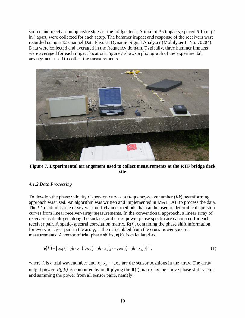
source and receiver on opposite sides of the bridge deck. A total of 36 impacts, spaced 5.1 cm (2 in.) apart, were collected for each setup. The hammer impact and response of the receivers were recorded using a 12-channel Data Physics Dynamic Signal Analyzer (Mobilyzer II No. 70204). Data were collected and averaged in the frequency domain. Typically, three hammer impacts were averaged for each impact location. Figure 7 shows a photograph of the experimental arrangement used to collect the measurements.

Figure 7. Experimental arrangement used to collect measurements at the RTF bridge deck

site

4.1.2 Data Processing

To develop the phase velocity dispersion curves, a frequency-wavenumber (f-k) beamforming approach was used. An algorithm was written and implemented in MATLAB to process the data. The f-k method is one of several multi-channel methods that can be used to determine dispersion curves from linear receiver-array measurements. In the conventional approach, a linear array of receivers is deployed along the surface, and cross-power phase spectra are calculated for each receiver pair. A spatio-spectral correlation matrix, R(f), containing the phase shift information for every receiver pair in the array, is then assembled from the cross-power spectra measurements. A vector of trial phase shifts, e(k), is calculated as

( ) ( ) ( ) ( )[ T21 exp , ,exp ,exp Nxjkxjkxjkk ⋅−⋅−⋅−= Le ] , (1)

where is a trial wavenumber and are the sensor positions in the array. The array output power, P(f,k), is computed by multiplying the R(f) matrix by the above phase shift vector and summing the power from all sensor pairs, namely:

k Nxxx ,,, 21 L

10

( ) ( ) ( ) ( )kfkkfP eRe , H= , (2)

where H denotes the Hermitian transpose. The output power value reaches its maximum value at the wavenumber(s) of the propagating waves. The phase velocity is then computed from the wavenumber and frequency as

kfVRπ2

= . (3)

In this study, the linear receiver array was assembled using one receiver location and stepping the source away from the receiver at fixed increments. The cross-power spectrum was measured between the source and receiver for each impact, and the spatio-spectral correlation matrix was assembled for each simulated receiver spacing. Figure 8 shows an example of the phase velocity–frequency contour plot developed from this processing procedure. The peaks in the plot represent the experimental dispersion curve.

Figure 8. Phase velocity–frequency contour plot for Case 1: Vertical impact with vertical

sensor; source and receiver on same side

4.2 Experimental Results

Data were collected at this site using a variety of source-and-receiver combinations. The results from the experimental studies are presented below and are compared to the theoretical dispersion curves calculated for this site. The theoretical dispersion curves were calculated based on a measured deck thickness of 20.32 cm (8 in.).

11

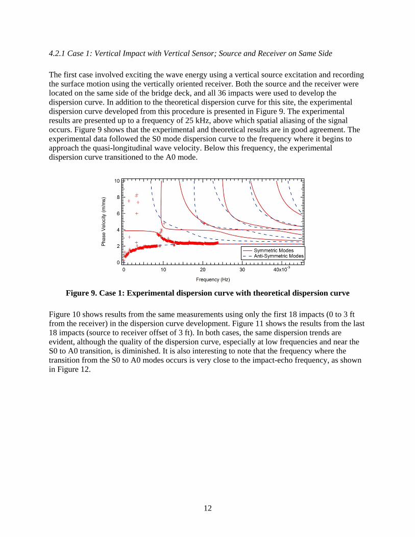
4.2.1 Case 1: Vertical Impact with Vertical Sensor; Source and Receiver on Same Side

The first case involved exciting the wave energy using a vertical source excitation and recording the surface motion using the vertically oriented receiver. Both the source and the receiver were located on the same side of the bridge deck, and all 36 impacts were used to develop the dispersion curve. In addition to the theoretical dispersion curve for this site, the experimental dispersion curve developed from this procedure is presented in Figure 9. The experimental results are presented up to a frequency of 25 kHz, above which spatial aliasing of the signal occurs. Figure 9 shows that the experimental and theoretical results are in good agreement. The experimental data followed the S0 mode dispersion curve to the frequency where it begins to approach the quasi-longitudinal wave velocity. Below this frequency, the experimental dispersion curve transitioned to the A0 mode.

Figure 9. Case 1: Experimental dispersion curve with theoretical dispersion curve

Figure 10 shows results from the same measurements using only the first 18 impacts (0 to 3 ft from the receiver) in the dispersion curve development. Figure 11 shows the results from the last 18 impacts (source to receiver offset of 3 ft). In both cases, the same dispersion trends are evident, although the quality of the dispersion curve, especially at low frequencies and near the S0 to A0 transition, is diminished. It is also interesting to note that the frequency where the transition from the S0 to A0 modes occurs is very close to the impact-echo frequency, as shown in Figure 12.

12

Figure 10. Case 1: Experimental dispersion curve (with theoretical dispersion curve) for

first 18 impacts at 0 to 0.91 m (0 to 3 ft)


last 18 impacts at 0.91 to 1.83 m (3 to 6 ft)

Figure 12. Impact-echo measurement with 2.54 cm (1 in.) source-receiver spacing

13

4.2.2 Case 2: Vertical Impact with Vertical Sensor; Source and Receiver on Opposite Sides

The second case involved repeating the measurements described above but with the source and receiver located on opposite sides of the bridge deck. This simulates the case where sensors are placed on the underside of a bridge deck and energy is excited from the surface. Again, the energy was excited with a vertical impact and detected with a vertically oriented accelerometer. The experimental dispersion curve was generated using all 36 impacts, as shown in Figure 13. The dispersion image is nearly identical to the image in the case with the source and receiver on the same side of the bridge deck. Figure 14 shows the dispersion image generated using the first 18 impacts, and Figure 15 shows the dispersion curve obtained using the last 18 impacts. In both cases, the same dispersion trend is observed, but the quality of the dispersion curve is degraded, and the transition between the S0 and A0 modes is not as clear.




14



4.2.3 Case 3: Vertical Impact with Radial Sensor; Source and Receiver on Same Side

Case 3 involved repeating the measurements made in Case 1 by exciting the wave energy using a vertical source but recording the surface motion using the receiver oriented in the radial direction. It was expected that the results for this setup would be similar to those obtained with the vertical orientation. The source and receiver were once again located on the same side of the bridge deck, and all 36 impacts were used to develop the dispersion curve. Figure 16 presents the experimental dispersion curve developed from this procedure, along with the theoretical dispersion curve for this site. In this case, the quality of the dispersion curve is not as good as when the vertical sensor was used. The transition between the A0 and S0 modes is not clear and appears to follow a single, continuous trend. The dispersion image from the first 18 impacts shows a more distinct separation between the A0 and S0 modes, as shown in Figure 17. Similar results were obtained when the final 18 impacts are used, as shown in Figure 18. Based on these results, it appears that the vertical sensor is a slightly better choice for developing the dispersion image.


15





4.2.4 Case 4: Vertical Impact with Radial Sensor; Source and Receiver on Opposite Sides

For Case 4, the measurements of Case 3 were repeated using an impact on the opposite side of the bridge deck. A vertical impact and radial sensor were used in this case. Figure 19 shows the dispersion image from all 36 impacts, and Figures 20 and 21 show the results from the first and last 18 impacts, respectively. The results are similar to those for the source and receiver on the same side of the deck.

16






17

4.2.5 Case 5: Transverse Horizontal Impact with Transverse Sensor; Source and Receiver on Same Side

The fifth case involved exciting horizontally polarized shear waves (SH) using a transverse impact source and recording the motion using a transversely oriented receiver. Using all 36 impacts to develop the dispersion curve, Figure 22 compares the results to the theoretical dispersion curve. In this case, the experimental dispersion curve follows the first antisymmetric mode. As shown in Figure 4, the cutoff frequency for this mode is a function of the thickness of the concrete plate and could potentially be used to identify the thickness of concrete over a subsurface delamination.


horizontally polarized shear waves

4.2.6 Case 6: Transverse Horizontal Impact with Transverse Sensor; Source and Receiver on Opposite Sides

The last case involved exciting SH waves on one side of the concrete deck and measuring the motions on the other side. The dispersion image produced from this measurement is shown in Figure 23. The points above 14 kHz were greatly scattered and were removed from the plot. Below 14 kHz, the dispersion measurement is in good agreement with the measurement performed with all instrumentation on the surface.

18


horizontally polarized shear waves

The measurements performed at the RTF facility demonstrated the ability to detect and separate multiple Lamb wave modes using a single sensor and multiple impact locations. The generated dispersion images indicate it is possible to infer the Rayleigh wave velocity of the concrete from the high-frequency portion of the dispersion curve and the thickness of the concrete based on the dispersion characteristics. The next section describes performing similar measurements on simulated concrete defects.

19

5. EXPERIMENTAL STUDIES AT MIDWAY SITE

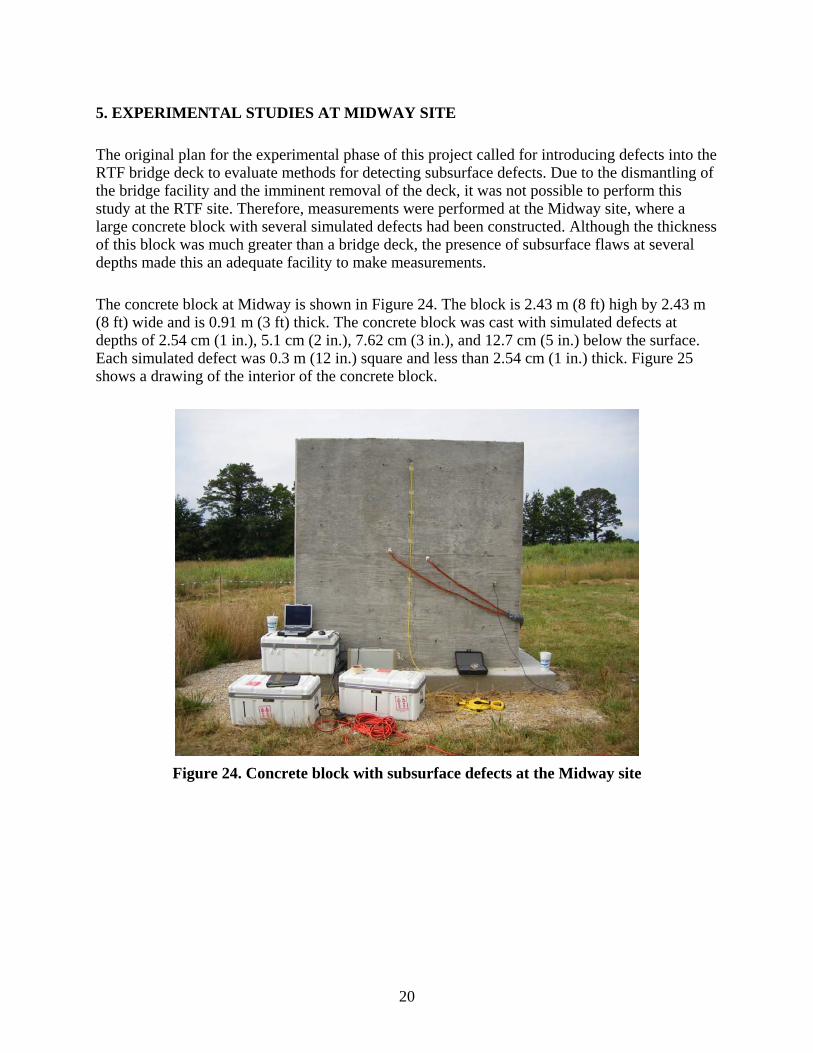
The original plan for the experimental phase of this project called for introducing defects into the RTF bridge deck to evaluate methods for detecting subsurface defects. Due to the dismantling of the bridge facility and the imminent removal of the deck, it was not possible to perform this study at the RTF site. Therefore, measurements were performed at the Midway site, where a large concrete block with several simulated defects had been constructed. Although the thickness of this block was much greater than a bridge deck, the presence of subsurface flaws at several depths made this an adequate facility to make measurements.

The concrete block at Midway is shown in Figure 24. The block is 2.43 m (8 ft) high by 2.43 m (8 ft) wide and is 0.91 m (3 ft) thick. The concrete block was cast with simulated defects at depths of 2.54 cm (1 in.), 5.1 cm (2 in.), 7.62 cm (3 in.), and 12.7 cm (5 in.) below the surface. Each simulated defect was 0.3 m (12 in.) square and less than 2.54 cm (1 in.) thick. Figure 25 shows a drawing of the interior of the concrete block.

Figure 24. Concrete block with subsurface defects at the Midway site

20

Figure 25. Drawing showing the interior of the Midway block and the locations of

subsurface defects in relation to the block. Numbers shown indicate the depth of the simulated delamination in inches.

5.1 Experimental Results from Midway Site

5.1.1 Measurements using Synthesized Array

To examine the influence of a defect on Lamb wave propagation, the measurement procedure performed at the RTF facility was repeated at the Midway site. First, measurements were taken along a section of the block that contained no defects using the same procedure employed at the RTF facility. The dispersion curve generated for this section using the vertical sensor is shown in Figure 26a, along with the theoretical dispersion curves for the 0.91 m (3 ft) thick concrete block. Next, the measurements were taken with the sensor located 0.36 m (1.2 ft) outside of the defect footprint. The hammer impacts were performed at 5.1 cm (2 in.) intervals, moving away from the sensor position and passing over and past the footprint of the defect. The objective of taking these measurements was to observe how the dispersion curves were influenced by the presence of the subsurface defect. The measurements were performed on the 5.1 cm (2 in.), 7.62 cm (3 in.), and 12.7 cm (5 in.) deep defects. The dispersion curves are presented with the control case of no defect in Figures 26b, 26c, and 26d. These figures show that only the 5.1 cm (2 in.) deep defect had any noticeable effect on the measured dispersion curves by causing a scattered response below about 10 kHz. The 7.62 cm (3 in.) and 12.7 cm (5 in.) deep defects caused no meaningful change in the dispersion curves as compared to the case with no subsurface flaws.

The radial component of motion was also used to develop dispersion curves over the three defects with similar results, as shown in Figure 27.

21

Measurements for SH (transverse) motions were next performed using the same procedure as described above. These measurements were performed on the 5.1 cm (2 in.) and 7.62 cm (3 in.) deep defects. The control case and the measurements from the two defects are shown in Figure 28. Other than increased scatter in the phase velocities, no meaningful change in the dispersion curves was observed for these cases.

(a)

(b)

(c)

(d)

Figure 26. Experimental dispersion curve developed from vertical motions for (a) control with no defects and (b) 5.08 cm (2 in.), (c) 7.62 cm (3 in.), and (d) 12.7 cm (5 in.) deep

defects. The theoretical dispersion curves for the control case are also shown.

22

(a)

(b)

(c)

(d)

Figure 27. Experimental dispersion curve developed from radial motions for (a) control

with no defects and (b) 5.08 cm (2 in.), (c) 7.62 cm (3 in.), and (d) 12.7 cm (5 in.) deep defects. The theoretical dispersion curves for the control case are also shown.

23

(a)

(b)

(c)

Figure 28. Experimental dispersion curve developed from SH motions for (a) control with

no defects and (b) 5.08 cm (2 in.) and (c) 7.62 cm (3 in.) deep defects. The theoretical dispersion curves for the control case are also shown.

5.1.2 Single Sensor Measurements

A series of measurements were performed to examine how the wave’s frequency content changed as it passed through the concrete containing the defects. In this case, the transfer function for the hammer impact and receiver on opposite sides of the void was calculated and compared to the case with no defect. These measurements were taken for the case of a vertical impact recorded with a vertical and a radial sensor, as well as the case of a transverse impact recorded with a transversely oriented sensor.

As might be expected, the frequency content of the wave was altered as it passed through the region containing the defect. For example, Figure 29 shows the results of an impact-echo measurement performed directly on the 12.7 cm (5 in.) defect using a vertically oriented sensor placed on the void and a vertical hammer impact 2.54 cm (1 in.) away. The transfer function between the hammer and the sensor shows a clear frequency peak at 14.49 kHz, which is consistent with a void at a depth of 12.7 cm (5 in.) and a compression wave velocity of 3,700 m/s using the typical impact-echo relationship

24

fVD*2

= , (4)

where D is the depth to the flaw, V is the compression wave velocity, and f is the measured frequency. A measurement was then taken by recording the transfer function between the hammer impact and a sensor located on opposite sides of the defect and separated by 0.97 m (3 ft 2 in.). The distance from the hammer to the near edge of the defect was 45.7 cm (18 in.), and the distance from the far edge of the defect to the sensor was 20 cm (8 in.). Figure 30 shows the transfer function recorded between the hammer and a radially oriented receiver, along with the transfer function recorded with the same measurement setup performed in a control area. This figure shows that frequencies near the impact-echo resonant frequency were amplified relative to the control. Results from the same measurement setup (hammer and receiver separated by 0.97 m and spanning the defect) performed on a 7.6 cm (3 in.) deep defect are shown in Figure 31. In this case, a frequency peak at 26 kHz was observed, which is close (within 10 %) to the value that is expected for an impact-echo measurement performed on this defect. These results demonstrate the potential to detect a defect from changes in the frequency content of waves propagating through the region containing the defect. Further studies are needed to validate the effectiveness of this approach.

Figure 29. Impact-echo measurements recorded over the defect at a depth of 12.7 cm (5 in.)

25

Figure 30. Transfer function recorded between hammer and radially oriented sensor separated by 0.97 m with a 12.7 cm deep defect present. The transfer function for the

control is also shown.

Figure 31. Transfer function recorded between hammer and radially oriented sensor separated by 0.97 m with a 7.6 cm deep defect present. The transfer function for the

control is also shown.

26

6. CONCLUSIONS

This research investigated the implementation of stress-wave–based NDE technologies to detect defects in concrete bridge decks. The ultimate objective is to develop new techniques to reliably and economically evaluate the deck condition. Measurements of stress wave propagation performed on a full-scale bridge deck demonstrated the ability to effectively detect and separate Lamb-wave modes using a single sensor and multiple impact locations. Measurements performed using vertical, radial, and transverse sensors yielded results that were consistent with the theoretical modes of Lamb wave propagation for the concrete deck. These measurements indicate the ability to determine both the Rayleigh wave velocity and the thickness of the concrete deck. Successful measurements were also performed with the source and receiver on opposite sides of the deck, as well as using horizontally polarized shear waves.

Field testing of this approach was performed over simulated defects in concrete at several depths below the surface. The results from field testing defects at three depths did not clearly indicate the presence or depth of the defect. A second approach was investigated, examining the potential to detect changes in the amplitude and frequency content of Lamb waves passing through the region containing the defect. Results from these measurements indicate amplification of energy in a frequency range indicative of the depth of the defect.

27

7. RECOMMENDATIONS FOR FUTURE STUDIES

Due to the demolition of the full-size bridge test facility prior to the completion of this project, it was not possible to perform measurements of wave propagation over subsurface flaws under ideal conditions. Although the testing on the concrete block provided some useful results, it is recommended that future studies focus on performing measurements on synthetic or real flaws in a full-size deck slab. This will minimize interference from waves reflected off of boundaries and better simulate expected conditions in the field.

The practical implementation of a stress-wave–based method will require the deployment of an affordable array of sensors. Therefore, it is also recommended that future work focus on studying the performance of inexpensive piezoelectric-film sensor arrays that could be attached to the underside of the deck.

28

29

REFERENCES

Alleyne, D. N. and Cawley, P. (1992). “The Interaction of Lamb Waves with Defects.” IEEE Trans.Ultrason., Ferroelectrics Freq. Control 39, 381–97.

Alt, D. and Meggers, D. (1996). “Determination of Bridge Deck Subsurface Anomalies by

Infrared Thermography and Ground Penetrating Radar: Polk-Quincy Viaduct I-70, Topeka, Kansas.” Report No. FHWA-KS-96-2, Kansas Dept of Transportation, September.

Jung, Y. C., Kundu, T., and Ebsani, M. (2001). "Internal Discontinuity Detection in Concrete by Lamb Waves." Mater. Eval., 59, 418–423. Kanno, T, Hara, S., and Takeichi, M. (2000). “In Service NDI for Delamination of Rehabilitated

RC Slab.” Proceedings, 15th World Conference on Non-Destructive Testing, Roma Italy, Oct.

Luangvilai, K., Punurai, W. and Jacobs, L.J. (2002). “Guided Lamb Wave Propagation in Composite Plate/concrete Component.” Journal of Engineering Mechanics, 128(12), pp

1337–1341. Na, W.B., Kundu, T., and Ehsani, M.R. (2003). “Lamb Waves for Detecting Delamination

Between Steel Bars and Concrete.” Computer-aided Civil Infrastruct. Eng., 18, 57–62. Pavlakovic, B. and Lowe, M. (2003). User’s Manual for Disperse: A System for Generating

Dispersion Curves. Ryden, N., Park, C.B., Ulriksen, P., and Miller R.D. (2003). “Lamb Wave Analysis for Non-

Destructive Testing of Concrete Plate Structures.” Proceedings of the 9th Meeting Environmental and Engineering Geophysics Society European Section (EEGS-ES), Prague, Czech Republic.

Scott, M., Rezaizadeh, A., Delahaza, S., Moore, M.E., Washer, G.A. (2003). “A Comparison of

Nondestructive Evaluation Methods for Bridge Deck Assessment.” NDT&E International, Vol. 36, April, p. 245-255.

Bridge Deck Integrity Measurements for Asset … Deck Integrity Measurements for Asset Management...

Documents

Transcript of Bridge Deck Integrity Measurements for Asset … Deck Integrity Measurements for Asset Management...